HAL Id: hal-00908450
https://hal.archives-ouvertes.fr/hal-00908450
Submitted on 23 Nov 2013
HAL is a multi-disciplinary open access
archive for the deposit and dissemination of
sci-entific research documents, whether they are
pub-lished or not. The documents may come from
teaching and research institutions in France or
abroad, or from public or private research centers.
L’archive ouverte pluridisciplinaire HAL, est
destinée au dépôt et à la diffusion de documents
scientifiques de niveau recherche, publiés ou non,
émanant des établissements d’enseignement et de
recherche français ou étrangers, des laboratoires
publics ou privés.
Multiple Compressive Projection Measurement for
Stepped Frequency Radar
Yun Lu, Christoph Statz, Sebastian Hegler, Wolf-Stefan Benedix, Valérie
Ciarletti, Dirk Plettemeier
To cite this version:
Yun Lu, Christoph Statz, Sebastian Hegler, Wolf-Stefan Benedix, Valérie Ciarletti, et al.. Multiple
Compressive Projection Measurement for Stepped Frequency Radar. 2nd International Workshop on
Compressed Sensing Applied to Radar (CoSeRa 2013), Sep 2013, Bonn, Germany. �hal-00908450�
Multiple Compressive Projection Measurement for
Stepped Frequency Radar
Yun Lu
∗, Christoph Statz
∗, Sebastian Hegler
∗, Wolf-Stefan Benedix
∗, Valérie Ciarletti
†, Dirk Plettemeier
∗ ∗Chair for RF Engineering, Technische Universität Dresden, Germany, Email: [email protected]†LATMOS/CNRS/IPSL/UVSQ, 78280 Velizy, France, Email: [email protected]
Abstract—In modern communication and measurement sys-tems, signal detection and estimation play a major role. Actually, the above two terms can be considered as one issue, e.g. pure detection by densely listing all possible diversites. The penalty is however the system complexity. Up to now, a lot of work have been invested, especially the recent compressed sensing (CS) technique [1], which is a subtle mathmatic application in practice and leads to a great sucess in signal detection both for communication and measurement, e.g. radar technique. In spite of this radical progress there are still a lot of open problems. One of them is the "noise" including background noise and non-ideal signal modelling, which is not just a problem for CS but a general difficulty for signal processing. Although there are many sophisticated recovery algorithms developed to cope with noise, the performance will be usually impacted by inaccurate noise estimation or modelling error. In this paper, we will analyti-cally describe the multiple compressive projection measurement (mCPM1 or MCPM) introduced in [2]. Both theoretical analysis and numerical evaluations show that mCPM is a promising measurement system.
I. INTRODUCTION
Suppose we have some target signal spanned in a particular frame Φ and provide a generative form
t = Φw + ξ, (1)
wheret∈ Rnis the vector of targets, Φ
∈ Rn×dis a frame of
d diversities that have been assumed, w is a vector of unknown weights, and ξ is Gaussian noise. The goal is to estimate w given t and Φ. Obviously, the maximum likelihood (ML) solution is very effective, if the dimension of w is smaller than that of the signal, i.e. n > d. In case of n < d, which is said to be underdetermined, a sparse w is required for a unique solution. Those problems can be handled by a general Bayesian framework [3]. An accurate result can be obtained if precise Φ and a reasonable estimation about ξ are available. Unfortunately, this is usually not the case in practice. That means, mostly we get only an estimation about Φ, denoted as
ˆ
Φ, as well as ξ. Thus, even without noise ξ we still cannot get the exact solution. To combat the noise ξ, which is usually non-sparse in Φ, we introduced themCPM. By using the restricted isometry property (RIP) for both sparse and non-sparse signal as well as the multi-correlation function (MCF) [4], the noise term in (1) can be well suppressed without exact information about the noise level in the channel. This work will focus on
1The special case is m= 1 as the conventional CS.
the general signal sensing2 of stepped frequency radar (SFR)
detecting sub-surface objects.
A. Organisation
The remaining of the paper is organised as follows: The Section II introduces the property of underdetermined linear systems und their solutions. Then, the theoretic detection behavior in compressive domain will be presented in Section III. In Section IV we will introduce the MCF as well as its combination with CS, termed asmCPM. The basic properties ofmCPM will be discussed. After that, we apply the mCPM in SFR and formulate new measurement approach for better performance. Finally, the summary and future work are pre-sented.
II. UNIQUE SOLUTION
Observing (1) with n < d, there are infinite solutions due to the fact that there are some linearly dependent diversity columns in Φ. In [5] the author gave a sparse condition in the sense of linear algebra for a unique solution, which was derived by clearly distinguishing two different unknown weightsw1andw2. That means, the difference of δ= w1−w2
must be uniquely detectable with respect to (1). In other words, δ is not allowed to lie in the null space of Φ, i.e. Φδ= 0. Thus, the columns controlled by δ, i.e. Φδ ∈ Rn×mδ and mδ ≤ n,
have to be linearly independent. Because of the randomness of δ in practice, Φδ ranges over the whole Φ. Finally, the number
of non-zero entries in δ, denoted as $δ$0 := |supp(δ)| and supp(δ) = {j : δj %= 0}, have to be smaller than the spark,
which denotes the least number of linearly dependent columns in Φ. Formally,
spark(Φ) = min
w"=0$w$0 subject to
Φw = 0. (2)
Furthermore, observing δ, we will get the maximal $δ$0 if weights w1 andw2 are disjoint (extreme case). This means
$δ$0≤ $w1− w2$0
=$w1$0+$w2$0 for w1∩ w2=∅.
(3) Obviously, (3) must hold the following condition
max{$δ$0} < spark(Φ). (4)
Thus, for a general unknown weight w and $w$0 = K, we
have
max{$δ$0} ≤ 2K < spark(Φ). (5) At last, the unique solution is given by holding the condtion
K < spark(Φ)/2 and $w$0= K. (6)
The results in (6) can also be interpreted as: The vector δ still preserves its Euclidean distance approximately after linear projection, i.e. Φδ. In other words, it holds
$Φδ$22≈ $Iδ$ 2
2, (7)
whereI is the identity matrix. This means, the 2K-th normal-ized singular value of Φ is not far from unit, which essentially requires that Φδ behaves like an orthogonal system. Similar
results can also be found in Johnson-Lindenstrauss (JL) lemma [6]. The JL lemma is concerned with the following problem. Given a set of points in Rd, we would like to embed these
points into a lower-dimensional Euclidean space Rn (n < d) while approximately preserving the relative distances between any two of these points. Let #∈ (0, 1) be given. For every set Q of #(Q) points in Rd, ifn is a positive integer such thatˆ
ˆ
n > n0= O(ln(#(Q))/#2), there exists a Lipschitz mapping
f : Rd → Rn such that (1− #) ≤ $f(u) − f(v)$ 2 lnˆ 2 $u − v$2ld 2 ≤ (1 + #) (8) for all u, v ∈ Q. That means, the Lipschitz function f as an injective function and the corresponding l2-norm distance
ratio is bounded by 1 + #. The JL lemma leads directly to the restricted isometry property (RIP) in CS [1]: If matrix Φ ∈ Rn×d satisfies the RIP of orderK with a constant #∈ (0, 1), such that (1− #) $w$22≤ $Φw$22≤ (1 + #) $w$22 holds for all w ∈ !
K, then w is recoverable. Usually, w can be
obtained by maximum a posteriori (MAP) estimation like lp
-norm regularization and FOCUSS [8] solving: min$Φw − t$22+ λ$w$
p
p for 0≤ p ≤ 1. (9)
In addition to MAP estimation, the full Bayesian approach [3], e.g. sparse Bayesian learning (SBL), which seeks for the distribution mass, improves the detection performance dramatically. The basic cost function can be given as: L = log |Σt| + tTΣ−1t t, where Σt = σ2I + ΦΓΦT with
hyperpa-rameters Γ= diag(γ) controlling the variance of entries in w. However, its performance is still very sensitve to inaccurate noise estimation. In the next section we will introduce the mCPM method to cope with "noise" effect.
III. COMPRESSIVEDETECTOR ANDmCPM
A. Compressive Detector
To improve the detection performance in underdetermined framework, we have to exame the statistic behavior in com-pressive domain with respect to the original signal domain.
For example, to distinguish two hypotheses: H0: y = M ξ
H1: y = M (x + ξ)
(10) whereM ∈ RmM×n withm
M < n is a measurement matrix,
ξ∼ N (0, σ2Id) is i.i.d. Gaussian noise. Then, the distribution
of y can be given as f0(y) = exp"−1 2y TΣ My# |σ2M MT|−1/2(2π)mM/2 f1(y) = exp"−1 2(y− Mx) TΣ M(y− Mx)# |σ2M MT|−1/2(2π)mM/2 (11)
where ΣM = (σ2M MT)−1. Based on the likelihood ratio
test Λ(y) = f1(y)
f0(y) ≷
H1
H0 η, where η is given for particular
false alarm probability α= $
Λ(y)>ηf0(y)dy, we can get an
equivalent detector in a compressive domain3: ˆ
t := yT(M MT)−1M x. (12) It is easy to show that
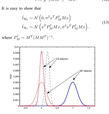
ˆ tH0∼ N % 0, σ2xTPM† M x & ˆ tH1∼ N % xTPM† M x, σ2xTPM† M x&. (13) wherePM† = MT(M MT)−1. −0.5 0 0.5 1 1.5 0 0.001 0.002 0.003 0.004 0.005 0.006 0.007 0.008 0.009 0.01 PDF CS detector MF detector
Figure 1. Distribution of hypotheses in detection domain by CS and MF.
If x = Φw and Φ = Id×d, the detection performance
in compressive domain is strongly depending on M . For a compressive detector, i.e.M is a wide matrix, x must live in the row span ofM with high probability, which is equivalent to require a sparse x. Furthermore, for a Gaussian matrix Mi ∈ RmM×n, xTPM†iMix is highly concentrated around
mM n $x$ 2 2. That is, E%xTP† MiMix & = mM n $x$ 2 2. (14) 3yT (M MT )−1 M x ≷H1 H0σ 2 log(η) +1 2x T MT (M MT )−1 M x. In case of M= I, then yT x ≷H1 H0σ 2 log(η) +1 2x T x.
Finally, with high probability we get the detection performance [9] PD(α)≈ Q % Q−1(α) −'SNRˆ & (15) withSNRˆ = mM n SNR and SNR=$x$ 2 2/σ2, andQ(z) = $∞
z exp(−u2/2)du.
1) Influence of compressive projection: Observing (15) the detection performance will be strongly affected by the dimension ratio of M , i.e. mM/n. In case of mM/n = 1,
the compressive projection is just an implementation of a traditional dectector (matched filter (MF), signal based). Then, we obtain the well-known detection performance:
PD(α)≈ Q
%
Q−1(α)−√SNR&. (16) For the case ofmM/n < 1, we could still get good recovery
performance, ifx lies in row span of M with high probability (vector based, e.g. CS, deteriorated detection performance depending on mM/n but still detectable).
2) Advantage of compressive projection: Compressive projection is not alwalys negative for information detection. As we know, the basic feasible solution to (9) is sparse, i.e. $w$0 ≤ n. However, in some cases like strong noise and coherent signals, the resulting solution still cannot avoid radical over-fitting. Although it can be partly compensated by choosing proper λ, the performance remains too sensitive to inaccurate λ. Besides, one is not allowed to set the λ too large (otherwise w disappears). Alternatively, observe the sparsity bound of solution from (9), it is limited by the row dimension n of Φ. In other words, we can reduce the row dimension to be an appropriate value in need for avoiding radical over-fitting regardless of recovery algorithms. Mathematically,
min$M (Φw − t)$22+ λ$w$pp for 0≤ p ≤ 1. (17) If x lies in the row span of M in high probability, the obtained sparser solution (local optimal solution) usually in-cludes weights w or at least part of them (in critical situa-tion). This sparsity controlling, i.e. $w$0 ≤ mM < n with
M ∈ RmM×n
and Φ ∈ Rn×d, excludes the over-fitting in unfavorable situation dramatically, since over-fitting usually needs particular amount of non-zero entries in solution. Thus, we expect the compressive detector having better performance against over-fitting than that of traditional detector in particular circumstance, namely requiring that reduction of n will not result in severe detection performance deterioration4. Yet, a solution without strong over-fitting is not enough for stable detection. Recall that the sparser solution by compressive detector has possibly only part of weightsw. To cope with this problem we will introduce the principle of multi-correlation function (MCF).
4The row dimension of matrix gives an upper bound of sparsity of feasible
solution regardless of recovery algorithms. To control sparsity one can also limit the number of iterations of sparse recovery algorithm (however, it sometimes hampers the convergence). An alternative way for over-fitting controlling is noise mitigation by column dimension extension. In this paper we mainly consider the case of compressive projection, i.e. row dimension reduction.
B. MCF
The MCF is basically an extension of the MF for achieving better correlation properties. The prime idea of MCF is based on the delay and multiply (DAM) property of m-code, which was later extended for generation of Gold codes. The DAM of m-code as well as Gold codes indicates that a transform of one m-code to its other phase delay or a transform of one Gold code to other family members can be realized by applying the DAM operation. Later, this property was applied to other Galois field (GF)-based codes. More information can be found in [10]. A paralell combination of several different correlation functions can result in much better correlation property than 1/√N given by the Sarwate lower bound, where N is the sequence length. Thus, it is very favorable for signal detection. Formally, the MCF can be given as
C(s) = 1 m m ( k=1 Fk = 1 mN m ( k=1 N −1 ( i=0 Ik(ui)Ik∗(vi+s), (18)
where m is the number of combinations, u and v are the original input sequences and the reference sequences, respec-tively. The code transform is given by the transform function I, e.g. DAM operation as above. The term Fk in (18) could be
any kind of "correlation" process or more generally recovery algorithm. The objective of combination ofm paralell results from Fk is achieving coherent combination or collecting the
partial result from single Fk with respect to information and
non-coherent combination of "noise" such that an even better detection scenario.
C. mCPM
The introduction of MCF into compressive detector, which is termed as mCPM here, could be very promising in our particular case and can also facilitate parameter adjustment with respect to information recovery in practice. Basically, mCPM consists of two steps: i) the first phase is actually a normal compressive projection and recovery (CPR) process by algorithm promoting sparse solution just as (17); ii) and the second phase is iteratively updating (combining) sparse solutions from each CPR by different compressive projections, e.g. different measurement matrix Mi, i.e. Θi = MiΦ, i
denotes thei-th iteration. Due to the underdetermined property y = M x = Θw with Θ ∈ Rn×d and n < d as well as
Θ holding the RIP with respect to w in high probability, the sparse solution w by single CPR includes w with highˆ probability while it provides randomness of noise in terms of their amplitudes and positions, since noise is usually non-sparse. Therefore, a combination of a series ofwˆi
wg= m ( i=1 ˆ wi (19)
can result in coherent combination of information components w and non-coherent combination of noise and thus a favorable detection scenario. Finally, the two close distribution modes of CS detector in Fig. 1 would be pulled apart from each other as well as their variance can be decreased depending
onM and m. A schematic illustration of mCPM is presented in Fig. 2. As a result, the radical over-fitting of the solution
no
end yes solution update sparse signal recovery compressive projection received datas; reference matrix
stop condition ?
Figure 2. mCPM
can be controlled by compressive recovery while its estimation deterioration is compensated by MCF principle. Fig. 3 shows
0.1 0.2 0.3 0.4 0.5 0.6 0.7 0.8 0.9 1 0 0.1 0.2 0.3 0.4 0.5 0.6 0.7 0.8 0.9 1 threshold probability Pd, MF+SBL Pf, MF+SBL Pd, mCPM+SBL Pf, mCPM+SBL Figure 3. SNR=3dB,"w"0 = 2, MF with Θ ∈ R 200×200 , mCPM with Θi∈ R50×200and m= 10
the false alarm probability (Pf) and detection probability (Pd) depending on different detection thresholds by normalizing the values within [0, 1]. Indeed, lines of Pf and Pd bymCPM are more favorable than that by MF.
Obviously, the performance ofmCPM is strongly depending on the compressive projections. An effective way for non-coherent combination of noise term in (19) requires that all compressive projection matrice Mi should be less correlated
with each other. Otherwise, the recovered noise term from two different iterations are similar and will also be coherently combined by (19), i.e. yield no contribution for distance expansion between signal term and noise term. Fig. 4 presents the estimation error e = $wg− w$2/$w$2 by mCPM with
m = 20 depending on row dimension of M . In case of small row dimension, the estimation error is relatively large, since the resulting reference matrix Θ does not hold the RIP con-dition with respect to w. For relatively large row dimension of M it also provides increased estimation error. The reason,
20 40 60 80 100 120 140 160 180 200 0.1 0.15 0.2 0.25 0.3 0.35 0.4 0.45 0.5 row dimension of M estimation error
Figure 4. Sparsity"w"0= 4, SNR=10dB, Θ = M Φ and Φ ∈ R 200×200 10 15 20 25 30 35 0.08 0.09 0.1 0.11 0.12 0.13 0.14 0.15 0.16 number of projections m estimation error
Figure 5. Reference matrix for mCPM Θi∈ R30×200, sparsity"w"0= 2,
SNR=10dB, the recovery algorithm is SBL, estimated noise factor is10−2.
as aforementioned, is that except the signal components a lot of recovered noise components also exhibit independence of randomM . This means, there are many noise components also live in the row span of the resulting reference matrix Θ, i.e. inefficiency of non-coherent noise combination. Besides, we
100−4 10−3 10−2 10−1
0.5 1 1.5
estimated noise factor
estimation error
MF+SBL, correlated signal
mCPM+SBL, correlated signal
MF+SBL, coherent signal
mCPM+SBL, coherent signal
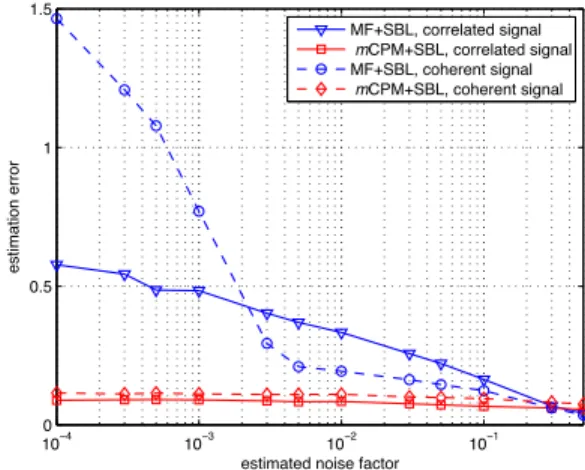
Figure 6. Reference matrix for mCPM Θi∈ R30×200, m= 30 and for
MF Θ∈ R200×200
can freely determine the number of projections m in mCPM for particular performance (see. Fig. 5). Setting a relatively large estimated noise factor the error by MF decreases fast, however, is not recommended, which is equivalent to set large λ in (9) and possibly results in the loss of information. This problem can be solved very well by mCPM, since mCPM still provides relatively small estimation error at low estimated noise factor (see Fig. 6).
IV. mCPMFOR STEPPED FREQUENCYRADAR(SFR)
A. SFR using CS
In the SFR radar [11], it observes the scene with a discrete set of frequencies and synthesizes the impulse in the frequency domain, and brings advantage of better accuracy. They pointed out that CS can be done in frequency domain by randomly measuring all Fourier coefficients. Thus, for rough detection it requires only a small amount of frequency measurements, which can first reduce the measurement time, and second save energy such that long-term activity is possible.
In this paper, we collect the frequency measurements from real circumstance and devices and process them directly in frequency domain. The connection to time domain for rang-ing information is simply the IFFT transform. Our objective vector, which indicates the ranging information, is wt. Its
corresponding vector in frequency domain is wf = F wt,
where F ∈ Cd×d is the FFT matrix and the dimension d
determines the required resolution in time domain. The prac-tical measurement for SFR is basically conducted in frequency domain and the number of frequency measurement points n is usually less than d. Thus, the actual obtained frequency
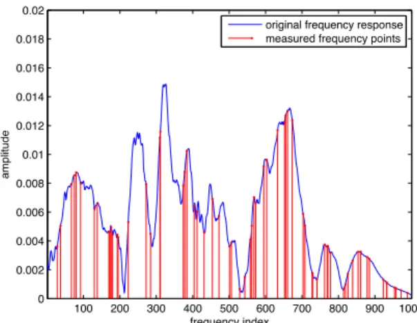
100 200 300 400 500 600 700 800 900 1000 0 0.002 0.004 0.006 0.008 0.01 0.012 0.014 0.016 0.018 0.02 frequency index amplitude
original frequency response measured frequency points
Figure 7. One practical example for randomly sub-sampling only 67 measurements in frequency domain, there are totally 1001 frequencies range from 500MHz to 3GHz.
vector is wn×1f r = Rwfd×1, where R = [In×n, 0n×(d−n)].
By using CS, we can futhermore reduce the number of frequency measurements per projection matrixM . Therefore, an underdetermined linear system can be constructed as
ˆ
wf r= M · R · F · wt= Θwt, (20)
where M determines which frequency point should be ac-tive (see Fig. 7). Finally, one needs to seek wt by solving
min{λ$wt$pp+$ ˆwf r− Θwt$2} with 0 ≤ p ≤ 1. This
non-20 40 60 80 100 120 140 160 180 200 0.2 0.3 0.4 0.5 0.6 0.7 0.8 0.9 1 relative error Nr. of frequencies
Figure 8. Relative error normed on the recovery error at sampling 10 frequencies.
convex optimization can be realized by FOCUSS or SBL approach. By given prior knowledge that the most reflections are clustered together we can limit the column dimension of Θ for better performance. Fig. 8 presents the relative recovery error by different number of frequency measurements. We can notice that it requires only about 50 frequencies for rough detection. In case of frequency number less than 30 the error increases dramatically. In practice, the SFR can work with following principle: For rough detection the radar can randomly (if necessary) and quickly measure just a few number of frequency points within a defined frequency range as presented in Fig. 7; In case of fine detection, the radar usually tries to collect as many frequency measurements as possible.
B. Full frequency measurement bymCPM
However, how to collect these frequency measurements plays a major role for stable and accurate information recovery. According to the conventional collection scheme, all defined frequency points will be measured once and processed. This approach, however, suffers from non-ideal signal modelling and inaccurate noise estimation especially for recovery algo-rithms, which are very sensitive to those effects (see Fig. 9).
Alternatively, the radar can work in mCPM mode, i.e. frequency measurements are collected partly, randomly and iteratively. Results from each iteration will be combined. This work mode, as discussed above, provides very stable recovery performance in a non-ideal scenario and facilitates parameter adjustment (see Fig. 10). The results in Fig. 9 and 10 are in the case that the influence of antenna pattern has not been calibrated. Nevertheless, the performance by mCPM is still well and better than the conventional work mode.
V. SUMMARY
In this paper we investigate the stepped frequency radar signal acquisition and processing by CS (or by generalized
mCPM). SFR using CS is a very promsing approach for long-term activity. By using mCPM5
, which can facilitate the fine measurement in practice, it provides even better performance than the conventional work mode. Basically, this work is not considering the feasibility and advantages of CS, rather a stable detection and estimation in noisy situation. The above results shows that even in full frequency mode, the mCPM mode is recommended.
As future work, we will focus on better energy distribution in frequency domain (frequency coding) such that giving better correlation properties in particular area in time domain. The results above are just based on the random selection principle. An optimal selection is still an open problem and also problem dependent. Further research direction is the noise mitigation (NM) by reference matrix extension. Generally [12],
min$M (Ψ ˜w− t)$22+ λ$ ˜w$ p
p for 0≤ p ≤ 1. (21)
where Ψ = [Φ, R] and M6
, R could be random matrix. The final solution is given by pruning the w, i.e. w˜ ∝ ˜wΦ,
where w˜Φ is the subvector related with Φ. The NM method
is expected to be more stable than row dimension reduction, since the change of row dimension is directly proportional to the recoverable sparsity, while the variation of column dimension is effected by a logarithm factor. More details will be discussed in our forthcoming paper.
Acknowledgment: WISDOM development and this research were sup-ported by funding from the French space agency CNES and from the German space agency DLR.
REFERENCES
[1] E. Candes; J. Romberg; T. Tao "Robust Uncertainty Principles: Exact Signal Reconstruction from Highly Incomplete Frequency Information" IEEE trans. inform theory, vol. 52, no. 2, pp. 489-509, Feb. 2006. [2] Y. Lu; C. Statz; S. Hegler; D. Plettemeier "Signal Sensing by Multiple
Compressive Projection Measurement", IRS 2013, Dresden.
[3] S. H. Ji; Y. Xue; L. Carin "Bayesian compressive sensing". Signal
Processing, IEEE Transactionson, 56(6):2346-2356, June 2008.
[4] Y. Lu; A. Finger "Novel multi-correlation differential detection for improving detection performance in DSSS," International symposium on
spread spectrum techniques and applications (ISSSTA), Taichung, Taiwan,
Oktober 2010.
[5] Donoho, D.L. and Elad, Michael "Optimally Sparse Representation from Overcomplete Dictionaries via l1-norm minimization". Proc. Natl. Acad.
Sci.USA March 4, 2003 100 5, 2197-2002, 2002.
[6] W. B. Johnson; J. Lindenstrauss "Extensions of lipschitz mappings into a hilbert space," In conference in modern analysis and probability, vol. 26 of Contemp. Mathematic, pp. 189-206, 1984.
[7] J. Tropp; A. Gilbert; M. Strauss "Algorithms for simultaneous sparse approximation. Part I: Greedy pursuit", Signal Processing, vol. 86, pp. 572-588, April 2006.
[8] I. Barrodale; F. Roberts "Applications of mathematical programming to lp approximation", Symposium on Nonlinear Programming, pp. 447-464, May 1970.
[9] L. L. Scharf "Statistical Signal Processing: Detection, Estimation, and Time Series Analysis", Addison-Wesley, 1991.
[10] Y. Lu; A. Finger "Method and apparatus for the differential multi-ple correlation in broadband ultrasonic location systems," (Patent) Nr.: EP10177353.9, 2010.
5It mainly focuses on stability by modifying the cost function. 6Mcan be identity matrix or random matrix.
[11] A. B. Suksmono; E. Bharata; A. A. Lestari "A compressive SFCW-GPR system". in proc. of 12th Int Conf. on Ground Penet Radar, Birmingham, pp. 16-19, 2008.
[12] Y. Lu, C. Statz, M. Mütze, S. Hegler, D. Plettemeier "Noise Mitigation and Extraction of Scatters in Acoustic Imaging by Compressed Sensing",
XVIII-th International Seminar/Workshop direct and inverse problems of
electromagnetic and acoustic wave theory, Lviv, Ukraine, 2013.
20 40 60 80 100 120 140 5 10 15 20 0 0.2 0.4 0.6 0.8 1 range index position
Figure 9. Recovery by full-sampling (1001 frequency points), MF+SBL, estimated noise factor is0.5 × 10−1
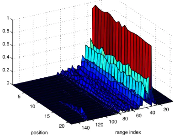
. Due to non-ideal noise estimation the performance is moderate 20 40 60 80 100 120 140 5 10 15 20 0 0.2 0.4 0.6 0.8 1 range index position
Figure 10. Recovery by randomly sub-sampling (average frequency points for each iteration is 80), mCPM+SBL with m= 30, estimated noise factor is0.5 × 10−1