HAL Id: hal-01509971
https://hal.inria.fr/hal-01509971v3
Submitted on 18 May 2018HAL is a multi-disciplinary open access
archive for the deposit and dissemination of sci-entific research documents, whether they are pub-lished or not. The documents may come from teaching and research institutions in France or abroad, or from public or private research centers.
L’archive ouverte pluridisciplinaire HAL, est destinée au dépôt et à la diffusion de documents scientifiques de niveau recherche, publiés ou non, émanant des établissements d’enseignement et de recherche français ou étrangers, des laboratoires publics ou privés.
Exact controllability in projections of the bilinear
Schrödinger equation
Marco Caponigro, Mario Sigalotti
To cite this version:
Marco Caponigro, Mario Sigalotti. Exact controllability in projections of the bilinear Schrödinger equation. SIAM Journal on Control and Optimization, Society for Industrial and Applied Mathemat-ics, 2018, 56. �hal-01509971v3�
Exact controllability in projections of the bilinear Schr¨
odinger
equation
∗Marco Caponigro† Mario Sigalotti‡§ May 18, 2018
Abstract
We consider the bilinear Schr¨odinger equation with discrete-spectrum drift. We show, for n∈ N arbitrary, exact controllability in projections on the first n given eigenstates. The controllability result relies on a generic controllability hypothesis on some associated finite-dimensional approxi-mations. The method is based on Lie-algebraic control techniques applied to the finite-dimensional approximations coupled with classical topological arguments issuing from degree theory.
1
Introduction
In this paper we study the controllability problem for the multi-input Schr¨odinger equation
idψ
dt(t) = (H0+ u1(t)H1+ . . . + up(t)Hp)ψ(t) (1)
where H0, . . . , Hpare self-adjoint operators on a Hilbert spaceH and the drift Schr¨odinger operator H0 (the internal Hamiltonian) has discrete spectrum. The control functions u1(·), . . . , up(·), representing
external fields, are real-valued and ψ(·) takes values in the unit sphere of H.
In recent years there has been an increasing interest in studying the controllability of the bilinear Schr¨odinger equation (1), mainly due to its importance for many applications such as laser spectroscopy or quantum information. The problem concerns the design of control laws (u1, . . . , up) steering the
system from a given initial state to a pre-assigned final state in a given time.
The controllability of system (1) is a well-established topic when the state space H is finite-dimensional (see for instance [15] and reference therein), thanks to general controllability methods for left-invariant control systems on compact Lie groups ([21, 20, 17, 16]).
We are interested here in the case in which H is infinite-dimensional. When the control operators
H1, . . . , Hp are bounded, it is known that the bilinear Schr¨odinger equation is not exactly controllable
(see [4, 35]). Hence, it is natural to look for weaker controllability properties such as approximate controllability or controllability between eigenstates of the Sch¨odinger operator. In certain cases it is possible to prove exact controllability in suitable functional spaces on a real interval (see [5, 6,
∗This work was supported by the project DISQUO of the DEFI InFIniTI 2017 by CNRS and the QUACO project by
ANR number 17-CE40-0007-01
†Conservatoire National des Arts et M´etiers, ´Equipe M2N, Paris, France (marco.caponigro@cnam.fr) ‡Inria (mario.sigalotti@inria.fr)
27]). In Rd, d > 1, the exact description of the reachable set seems a difficult task. However, approximate controllability results have been obtained with different techniques: adiabatic control ([1, 11]), Lyapunov methods ([25, 28, 29, 30]), and Lie-algebraic methods ([14, 8, 9, 13, 10, 7, 22, 31]). The Lie-algebraic approach developed in [14, 9, 13, 10] serves as basis for the analysis in this paper. The basic idea is to drive the system with control laws that are in resonance with spectral gaps of the internal Hamiltonian H0. The resonances are used to identify finite-dimensional dynamics which can be tracked with arbitrary precision by the infinite-dimensional system. In [10] we used this reduced finite dimensional dynamics to introduce the Lie–Galerkin Control Condition (see Definition 4 below), which ensures approximate controllability of (1) in the unit sphere of H. The condition applies for very degenerate spectra of the internal Hamiltonian H0 and also guarantees approximate operator controllability, approximate controllability in finer topologies, and tracking.
In this paper we go beyond approximate controllability and prove that the Lie–Galerkin Control Condition implies a stronger controllability property: exact controllability in projections. More pre-cisely, our main result, Theorem 3, states that given a Hilbert basis (ϕk)k∈N ofH made of eigenvectors
of H0, for every given n∈ N, initial condition ψin∈ H with ∥ψin∥ = 1, and final condition ψf ∈ H such that∥ψf∥ = 1 with ⟨ψf, ϕj⟩ ̸= 0 for some j > n there exists an admissible control t 7→ (u1(t), . . . , up(t))
such that the associated solution t7→ ψ(t) of (1) with ψ(0) = ψin satisfies⟨ΥuT(ψin), ϕj⟩ = ⟨ψf, ϕj⟩ for
every j = 1, . . . , n. Exact controllability in projections guarantees, for example, that given any initial condition ψin and any n∈ N, it is possible to steer in finite time ψinto the orthogonal complement of span{ϕ1, . . . , ϕn}. It also guarantees the possibility to implement exactly, in finite time, a Quantum
Random Number Generation protocol (see e.g., [23, 19]) with an infinite dimensional system. In the simplest protocol, for instance, the initial state is steered to a final state who has a probability of 1/2 to be measured in the ground state.
The idea of the proof of exact controllability in projections is the following. The Lie–Galerkin Control Condition provides controllability for any fixed finite-dimensional approximation while avoid-ing the transfer of population to higher energy levels for higher-dimensional approximations. This yields estimates on the difference between the dynamics of the finite-dimensional approximation and the original infinite-dimensional system. This fact combined with the continuity of the input-output mapping (see Assumption (A5)) and a topological degree argument ensures exact controllability in projections.
The hypothesis that the final condition ψf satisfies⟨ψf, ϕj⟩ ̸= 0 for some j > n cannot be removed.
Since, as we have already recalled, one cannot expect exact controllability tout court if the control operators H1, . . . , Hp are regular (e.g., continuous). The regularity of the control operators, and as
a consequence of the input-output mapping, is therefore an obstruction for the exact controllability while, on the other hand, continuity of the input-output mapping is an assumption needed for the application of the topological degree methods used in the proof of Theorem 3 below. In this sense the controllability in projections is the strongest general controllability property that one may expect in the framework of bounded control potentials.
2
Framework and main result
Let p ∈ N, δ > 0, and U = U1 × · · · × Up with either Uj = [0, δ] or Uj = [−δ, δ]. For simplicity
of notation we consider the bilinear control systems obtained by replacing the operators in (1) by
Definition 1. LetH be an infinite-dimensional Hilbert space with scalar product ⟨·, ·⟩ and A, B1, . . . , Bp
be (possibly unbounded) skew-adjoint operators on H, with domains D(A), D(B1), . . . , D(Bp). Let
us introduce the controlled equation
dψ
dt(t) = (A + u1(t)B1+· · · + up(t)Bp)ψ(t), u(t)∈ U. (2)
We say that A satisfies (A1) if the following assumption holds true.
(A1) A has discrete spectrum with infinitely many distinct eigenvalues (possibly degenerate).
Note that (A1) is true whenever A has compact resolvent. Denote by Φ a Hilbert basis (ϕk)k∈N of
H made of eigenvectors of A associated with the family of eigenvalues (iλk)k∈N and let L be the set
of finite linear combinations of eigenstates, that is,
L = ∪
k∈N
span{ϕ1, . . . , ϕk}.
We consider the following assumptions on the regularity of the control operators B1, . . . , Bp:
(A2) ϕk∈ D(Bj) for every k∈ N, j = 1, . . . , p;
(A3) A + u1B1+· · · + upBp :L → H is essentially skew-adjoint for every u ∈ U.
When (A, B1, . . . , Bp, Φ, U ) satisfies (A1) − (A2) − (A3) we define the solution of (2) as follows.
Definition 2. We say that u ∈ L∞([0, T ],Rp) is admissible for (2) if u(t) ∈ U for almost every
t ∈ [0, T ] and, for every ψ0 ∈ H, there exists ψ : [0, T ] → H such that ψ(0) = ψ0 the function
t7→ ⟨ψ(t), ϕk⟩ is absolutely continuous for every k ∈ N and satisfies
d
dt⟨ϕk, ψ(t)⟩ = −⟨(A + u1(t)B1+· · · + up(t)Bp)ϕk, ψ(t)⟩, (3)
for almost every t∈ [0, T ]. The function t 7→ ψ(t) is called solution of (2) with initial condition ψ0∈ H associated with the control u.
Assumption (A3) implies that the norm of the solutions given by Definition 2 is constant along the evolution. In particular it guarantees the uniqueness of solutions. We can therefore define the unitary propagator of (2), denoted by Υut, as follows.
Definition 3. Let u : [0, T ] → U be admissible for (2). The mapping [0, T ] ∋ t 7→ Υut where Υutψ0 is the evaluation at time t of the solution of (2) with initial condition ψ0 ∈ H associated with u, is called propagator of (2).
Let (A, B1, . . . , Bp, Φ, U ) satisfy (A1) − (A2) − (A3) and let U ⊂ L∞([0,∞), U). We say that
(A, B1, . . . , Bp, Φ, U,U) satisfies (A4) if
(A4) every u ∈ U is admissible.
Assumption (A4) holds true for the class of piecewise constant controls and, under suitable regu-larity conditions, for the class of smooth controls as detailed in the following two remarks.
Remark 1. Let (A, B1, . . . , Bp, Φ, U ) satisfy (A1) − (A2) − (A3) and let u(·) = (u1(·), . . . , up(·)) be a
p-tuple of piecewise constant controls on [0, T ] with value in U . Then u is admissible for (2) and the
propagator is given by
Υut = e(t−∑j−1l=1tl)(A+u
(j)
1 B1+···+u(j)p Bp)◦ · · · ◦ et1(A+u(1)1 B1+···+u(1)p Bp),
where∑jl=1−1tl≤ t < ∑j l=1tl and u(τ ) = (u (j) 1 , . . . , u (j) p )∈ U if ∑j−1 l=1 tl≤ τ < ∑j l=1tl. Indeed, since
⟨ϕn, et(A+u1B1+···+upBp)ψ0⟩ = ⟨e−t(A+u1B1+···+upBp)ϕn, ψ0⟩ , then t7→ ψ(t) = Υu
tψ0 satisfies (3) for almost every t∈ [0, T ].
Remark 2. Let u∈ C1([0, T ], U ) and B1, . . . , Bp be A-bounded with A-bound smaller than 1/δ in the
sense of [32, Section X.2], i.e.
• D(Bj)⊃ D(A),
• there exists a < 1/δ and b ∈ R such that for all ϕ ∈ D(A) one has ∥Bjϕ∥ ≤ a∥Aϕ∥ + b∥ϕ∥,
for every j = 1, . . . , p. Then by the Kato–Rellich theorem ([32, Theorem X.12]) and [32, Theorem X.70]
u is admissible for (2). If, moreover, ψ0 ∈ D(A) then t 7→ Υutψ0 satisfies (2) for every t∈ [0, T ]. We say that (A, B1, . . . , Bp, Φ, U,U) satisfies (A) if it satisfies (A1) − (A2) − (A3) − (A4) and the
following additional assumption.
(A5) The input-output mapping is continuous in the sense that if (un)n∈N ⊂ U and u ∈ U are such
that un → u in L1([0, T ]) as n → ∞ then Υunt ϕ tends to Υutϕ in H uniformly with respect to
t∈ [0, T ] as n → ∞ for every ϕ ∈ H.
Remark 3. In the case in which A satisfies (A1) and B1, . . . , Bp are bounded operators, assumptions
(A2), (A3) are clearly verified. Assumption (A5) is the consequence of [4, Theorem 3.6]. More general conditions on B1, . . . , Bp ensuring that (A5) holds true can be found for instance in [12, Section 2.3].
For n∈ N we denote by Πnthe projection ofH on the span of the first n eigenvectors of A, namely
Πn: H → H
ψ 7→ ∑nk=1⟨ϕk, ψ⟩ϕk.
When it does not create ambiguities we identify Im(Πn) = span{ϕ1, . . . , ϕn} with Cn. Given a linear
operator Q on H we identify the linear operator πnQπn preserving span{ϕ1, . . . , ϕn} with its n × n
complex matrix representation with respect to the basis (ϕ1, . . . , ϕn). We define
A(n)= ΠnAΠn and Bj(n)= ΠnBjΠn,
for every j = 1, . . . , p.
Let us introduce the set Σn of spectral gaps associated with the first n eigenvalues of A as
For every σ≥ 0, every m ∈ N, and every m × m matrix M, let
Eσ(M ) = (Ml,kδσ,|λl−λk|)ml,k=1,
where δ·,· denotes the Kronecker symbol. The n× n matrix Eσ(Bj(n)), j = 1, . . . , p, corresponds then
to the “selection” in Bj(n) of the spectral gap σ: the (l, k)-elements such that|λl− λk| ̸= σ are set to
0.
Define Ξn=
{
(σ, j)∈ Σn× {1, . . . , p} | (Bj)k,lδσ,|λl−λk|= 0, for every k = 1, . . . , n and l > n
}
. (4) The set Ξn can be seen as follows: If (σ, j)∈ Ξn then the matrix M =Eσ(Bj(n)) is such that
Eσ(Bj(N )) = ( M 0 0 ∗ ) for every N > n.
In particular span{ϕ1, . . . , ϕn} is invariant for the evolution of Eσ(Bj(N )) for every N > n. The spectral
gaps σ ∈ Ξn are, therefore, those for which the selectionsEσ(Bj(n)) define finite dimensional dynamics
of order n “decoupled” from the infinite dimensional evolution.
The main assumption of this paper, introduced in the definition below, is a Lie-algebraic condition on the set of the decoupled selections associated with the spectral gaps in Ξn.
Definition 4 ([10]). For every n∈ N define
Mn=
{
A(n)
}
∪{Eσ(Bj(n))| (σ, j) ∈ Ξnand j is such that (0, j)∈ Ξn
}
∪{Eσ(Bj(n))| (σ, j) ∈ Ξn, σ̸= 0, Uj = [−δ, δ]
}
.
We say that the Lie–Galerkin Control Condition holds if for every n0 ∈ N there exists n > n0 such that
LieMn⊇ su(n).
The Lie–Galerkin Control Condition is a sufficient condition for approximate controllability as stated in Theorem 1 below.
Definition 5. Let (A, B1, . . . , Bp, Φ, U,U) satisfy (A1) − (A2) − (A3) − (A4). We say that (2) is
approximately controllable by means of controls in U if for every ψ0, ψ1 in the unit sphere of H and every ε > 0 there exists u∈ U and T > 0 such that ∥ψ1− ΥuT(ψ0)∥ < ε.
Theorem 1 ([10, Theorem 2.6]). Let (A, B1, . . . , Bp, Φ, U ) satisfy (A1) − (A2) − (A3). If the Lie–
Galerkin Control Condition holds then system (2) is approximately controllable by means of piecewise constant controls.
Theorem 1 can be extended to the class of smooth controls as stated in Theorem 2 below. The proof of this result is given in Section 4.
Theorem 2. Let U be the set of C∞ functions with values in U and (A, B1, . . . , Bp, Φ, U,U) satisfy
(A1)−(A2)−(A3)−(A4). If the Lie–Galerkin Control Condition holds then system (2) is approximately
Our main result is the approximate controllability in projections as stated below. Theorem 2 is one of the main tools in its proof.
Theorem 3. LetU be either the set of piecewise constant functions with values in U or the set of C∞
functions with values in U . Let (A, B1, . . . , Bp, Φ, U,U) satisfy (A). Assume that the Lie–Galerkin
Control Condition holds. Then for every n ∈ N, ε > 0, for every initial condition ψin ∈ H with
∥ψin∥ = 1 and every final condition ψf ∈ H such that ∥ψf∥ = 1 and ∥Πn(ψf)∥ < 1, there exists
u : [0, T ]→ U, u ∈ U such that
Πn(ΥuT(ψin)) = Πn(ψf) and ∥ΥuT(ψin)− ψf∥ < ε.
2.1 The Lie–Galerkin Control Condition in examples
2.1.1 Non-resonant chain of connectedness
An example of easily verifiable condition in the case of single-input systems which implies the Lie– Galerkin Control Condition is given by the existence of a non-resonant chain of connectedness, as we recall below. Let p = 1 and call, for simplicity, B = B1. Let (A, B, Φ, U ) satisfy assumption (A1) − (A2) − (A3).
Definition 6 ([9]). A subset S of N2 couples two levels l, k in N, if there exists a finite sequence
( (s1 1, s12), . . . , (s q 1, s q 2) ) in S such that (i) s11 = l and sq2 = k;
(ii) sj2= sj+11 for every 1≤ j ≤ q − 1; (iii) ⟨ϕsj
1, Bϕs
j
2⟩ ̸= 0 for 1 ≤ j ≤ q.
S is called a connectedness chain for (A, B, Φ, U ) if S couples every pair of levels in N.
A connectedness chain is said to be non-resonant if for every (s1, s2) in S,|λs1− λs2| ̸= |λt1− λt2| for every (t1, t2) in N2\ {(s1, s2), (s2, s1)} such that ⟨ϕt2, Bϕt1⟩ ̸= 0.
Proposition 4. Assume that ⟨ϕl, Bϕk⟩ = 0 whenever l ̸= k and λl = λk. If (A, B, Φ, U ) admits a
non-resonant connectedness chain then the Lie–Galerkin Control Condition holds.
Proof. The first assumption in the statement of the proposition implies that 0∈ Ξn for every n. The
non-resonance condition on the eigenvalues implies that, for every n, Ξn= Σn. Hence
Mn= { A(n) } ∪{Eσ(B(n))| σ ∈ Σn } .
Since, moreover, E|λl−λk|(B(n)) has two nonzero entries if ⟨ϕl, Bϕk⟩ ̸= 0, the Lie–Galerkin Control
Condition follows easily from the existence of a connectedness chain (see, for instance the proof of [9, Proposition 3.1] for details).
Remark 4. As a consequence of Proposition 4, the Lie–Galerkin Control Condition is satisfied by a
generic single-input bilinear Schr¨odinger equation
i ˙ψ = (−∆ + V )ψ + uW ψ
on Ω bounded domain of RN and V and W are smooth functions from Ω → RN, see [24, Theorem 3.4].
2.1.2 Rotating bipolar molecule
Consider the control of the orientation of a rigid bipolar molecule in R3 modeled by the following Schr¨odinger equation on the unit sphere S2:
i∂ψ(θ, φ, t)
∂t =− ∆ψ(θ, φ, t)+
+ (u1(t) sin θ cos φ + u2(t) sin θ sin φ + u3(t) cos θ)ψ(θ, φ, t), (5) where θ, φ are the spherical coordinates, which are related to the Euclidean coordinates through the identities
x = sin θ cos φ, y = sin θ sin φ, z = cos θ,
while ∆ is the Laplace–Beltrami operator on the sphere S2 (called in this context the angular
mo-mentum operator ), i.e.,
∆ = 1 sin θ ∂ ∂θ ( sin θ ∂ ∂θ ) + 1 sin2θ ∂2 ∂φ2.
The wavefunction ψ evolves in the unit sphere S of H = L2(S2,C). A basis of eigenvectors of the
Laplace–Beltrami operator ∆ is given by the spherical harmonics Yℓm(θ, φ), which satisfy ∆Yℓm(θ, φ) =−ℓ(ℓ + 1)Yℓm(θ, φ).
The spectrum of A = i∆ is {−iℓ(ℓ + 1) | ℓ ∈ N}. Each eigenvalue −iℓ(ℓ + 1) is of finite multiplicity 2ℓ+1. The control operators B1, B2, B3are the multiplication operators by−i cos φ sin θ, −i sin φ sin θ,
−i cos θ, respectively, which are bounded.
For symmetry reasons, the system is not controllable if one the three control is constantly switched off. In particular, the argument of Proposition 4 does not apply directly.
The systems satisfies condition (A1) − (A2) − (A3). Assumptions (A4) and (A5), for piecewise constant or C1 smooth controls, follow from Remarks 1, 2, and 3. Equation (5) satisfies the Lie– Galerkin Control Condition as proved in [10, Lemma 3.2].
2.1.3 Quantum harmonic oscillator
The quantum harmonic oscillator is among the most important examples of quantum systems. Con-sider its controlled version (see, for instance, [26]), in which H = L2(R, C) and the equation (2) reads i∂ψ ∂t(x, t) = 1 2(−∆ + x 2)ψ(x, t) + u(t)xψ(x, t).
A Hilbert basis of H made of eigenvectors of A = −2i(−∆ + x2) is given by the Hermite functions (ϕn)n∈N, associated with the sequence (−iλn)n∈N of eigenvalues, where λn = n− 1/2. In the basis
(ϕn)n∈N, B1 = B =−ix is tri-diagonal since
⟨ϕj, Bϕk⟩ = i√k− 1 if j = k − 1, i√k if j = k + 1, 0 otherwise.
This system is known to be non-controllable, neither exactly nor approximately as proved in [26], while its Galerkin approximations of every order are [33].
In this example, for every n, Σn={0, 1, 2, . . . , n}, Ξn= Σn\ {1} and Eσ(B(n)) is the zero matrix
2.2 Strategy of the proof
The strategy of the proof of Theorem 3 splits into two main arguments. The first argument is used to formalize the decoupling which we mentioned as the intuition behind the definition of the setMn.
More precisely, for every n∈ N, we show that there exists a family Wn of n× n matrices having the
same Lie algebra asMn, which defines a control system inCnwhose trajectories can be approximated
arbitrarily well by the projection Πn of trajectories of (2). The second argument goes as follows: if n
is such that the Lie algebra generated byWn(or, equivalently, by Mn) is su(n), then for every point
of the unit sphere of Cn there exists a control law at which the endpoint map of the control system
defined byWn is a submersion. Then, by structural stability of submersions, it is possible to deduce
exact controllability in projection of (2).
The first of the two arguments mentioned above spans Sections 3 and 4 and allows, in particular, to provide a proof of Theorem 2. It consists in three steps: an averaging result used to compare (up to phases) the flow of a matrix ofWn with a trajectory of (2) corresponding to a control in resonance
with one of the frequencies in Ξn(see Lemma 6), a construction allowing to concatenate the averaging
arbitrarily many times (see Proposition 8), and a concluding phase tuning step (see Lemma 9).
3
Finite-dimensional approximations of infinite-dimensional
propa-gators
In this section we introduce an auxiliary control system whose solutions are, up to phases, trajectories of (2), as showed in Lemma 5 below.
For t, u1, . . . , up ∈ R set Θ(t, u) = Θ(t, u1, . . . , up) = e−tA(u1B1+· · · + upBp)etA, which is a linear
operator from L to H. Note that
Θ(t, u1, . . . , up)jk =⟨ϕk, Θ(t, u1, . . . , up)ϕj⟩ = ei(λk−λj)t(u1(B1)jk+· · · + up(Bp)jk) .
Consider the nonautonomous control system ˙
y(t) = Θ(t, u1(t), . . . , up(t))y(t). (6)
Admissible solutions of (6) are, as in Definition 2, absolutely continuous functions y : [0, T ] → H satisfying
d
dt⟨ϕn, y(t)⟩ = −⟨Θ(t, u1(t), . . . , up(t))ϕn, y(t)⟩, (7)
for any n∈ N and for almost every t ∈ [0, T ].
Lemma 5. Let u ∈ U. Then u is admissible for (6) and the corresponding admissible solution
y : [0, T ]→ H associated with the initial condition y(0) satisfies
Υut(y(0)) = etAy(t), for every t∈ [0, T ].
Proof. The function
satisfies d dt⟨ϕn, y(t)⟩ = d dte itλn⟨ϕ n, Υut(y(0))⟩
= iλneitλn⟨ϕn, Υut(y(0))⟩ + eitλn
d dt⟨ϕn, Υ
u t(y(0))⟩
= iλneitλn⟨ϕn, Υut(y(0))⟩ − eitλn⟨(A + u1(t)B1+· · · + up(t)Bp)ϕn, Υut(y(0))⟩
=−eitλn⟨(u1(t)B1+· · · + up(t)Bp)ϕn, etAy(t)⟩
=−⟨Θ(t, u1(t), . . . , up(t))ϕn, y(t)⟩,
for every n∈ N and for almost every t ∈ [0, T ].
The following lemma is inspired by [13, Theorem 1]. Here we denote by ∥ · ∥L(E,H) the norm of linear operators from a subspace E of H to H.
Lemma 6. Let n∈ N, σ > 0, j ∈ {1, . . . , p}, ν0 and ν1 in R, and a, b ∈ R such that 0 < a < b. For
every N > n let ωN = (0, . . . , 0 | {z } j−1 , vN, 0, . . . , 0 | {z } p−j
) : R → Rp be a periodic function of period T = 2π/σ,
such that ∫ T 0 vN(t)dt = ν0, ∫ T 0 vN(t)eiσtdt = ν1, (8) and ∫ T 0
vN(t)eimσtdt = 0, for every m≥ 2 such that mσ ∈ ΣN. (9)
Assume that one of the following three conditions is satisfied: (i) (σ, j) and (0, j) are in Ξn; (ii)
(σ, j)∈ Ξn and ν0 = 0; (iii) (0, j)∈ Ξn and ν1 = 0. Assume, moreover, that ωN/K is admissible for
every N ∈ N and every K ∈ N large enough. Then
lim N→∞Klim→∞∥Υ τ ωN/K KT − e KT Aexp(τ (ν 0E0(Bj(n)) + ν1Eσ(B(n)j )))∥L(Πn(H),H)= 0,
uniformly with respect to τ ∈ [a, b], where exp(τ(ν0E0(Bj(n)) + ν1Eσ(B(n)j ))) : Cn → Cn is identified
with an operator on H.
Proof. Step 1. Fix, for now, N > n and consider the Galerkin approximation of order N of system (6),
namely the system associated with Θ(N )(t, u) = ΠNΘ(t, u)ΠN. Then, for every s≤ t and τ ∈ [a, b], −→ exp ∫ Kt Ks Θ(N ) ( r,τ ω N(r) K ) dr =exp−→ ∫ t s Θ(N )(Kr, τ ωN(Kr)) dr =exp−→ ∫ t s e−rKA(N )τ vN(Kr)Bj(N )erKA(N )dr, (10)
where the notation exp is used to denote the chronological exponent, see [3]. We claim that−→ ∫ t s e−rKA(N )vN(Kr)Bj(N )erKA(N )dr→ t− s T ( ν0E0(Bj(N )) + ν1Eσ(Bj(N )) ) (11)
as K → ∞, uniformly with respect to s, t ∈ [0, T ]. Indeed, this follows from (9) and the fact that for every σ′ ∈ R \ σZ 1 K ∫ Kt Ks vN(r)eiσ′rdr→ 0
as K → ∞, as it can be seen by developing vN in Fourier series.
Hence by (10), (11), and averaging arguments (see, for instance, [3, Lemma 8.2]) we deduce that
−→ exp ∫ Kt Ks Θ(N ) ( r,τ ω N(r) K ) dr→ exp ( (t− s)τ T ( ν0E0(Bj(N )) + ν1Eσ(Bj(N )) )) (12) as K → ∞, uniformly with respect to s, t ∈ [0, T ] and τ ∈ [a, b].
Step 2. Let
y(t) = e−tAΥτ ωt N/K(ψ), for ψ∈ Πn(H). By Lemma 5, y(t) is a solution of (6).
By variation of constants formula and since ΠNΘ(s, u)(I− ΠN) is an operator uniformly bounded
with respect to s∈ R and u ∈ U, we deduce from (7) that Πny(t) = Πn exp−→ ∫ t 0 Θ(N ) ( s,τ ω N(s) K ) ds (ψ) + Πn ∫ t 0 ( −→ exp ∫ t s Θ(N ) ( r,τ ω N(r) K ) dr ) ΠNΘ ( s,τ ω N(s) K ) (I− ΠN)y(s)ds.
We are left to prove that limN→∞limK→∞Πne−KT AΥτ ω N/K
KT Πn= exp(ν0E0(Bj(n)) + ν1Eσ(Bj(n)))
uni-formly with respect to τ ∈ [a, b]. Indeed, by unitarity of the evolution of (6), this also implies that lim
N→∞Klim→∞(I− Πn)e
−KT AΥτ ωN/K
KT Πn= 0,
uniformly with respect to τ ∈ [a, b]. By (12), for every N > n we have that
lim K→∞Πn −→ exp ∫ KT 0 Θ(N ) ( s,τ ω N(s) K ) ds Πn= exp(τ (ν0E0(Bj(n)) + ν1Eσ(Bj(n)))),
uniformly with respect to τ ∈ [a, b]. Hence, we are left to prove that for every ε > 0 and every N large enough one has
lim sup K→∞ ∥Πn ∫ KT 0 ( −→ exp ∫ KT s Θ(N ) ( r,τ ω N(r) K ) dr ) ΠNΘ ( s,τ ω N(s) K ) (I−ΠN)e−sAΥτ ω N/K s dsΠn∥ < ε,
uniformly with respect to τ ∈ [a, b]. Notice that ∫ KT 0 ( −→ exp ∫ KT s Θ(N ) ( r,τ ω N(r) K ) dr ) ΠNΘ ( s,τ ω N(s) K ) (I− ΠN)e−sAΥτ ω N/K s ds = ∫ T 0 ( −→ exp ∫ KT Ks Θ(N ) ( r,τ ω N(r) K ) dr ) ΠNΘ ( Ks, τ ωN(Ks))(I− ΠN)e−KsAΥτ ω N/K Ks ds.
We are going to prove, therefore, that for every ε > 0 and every N large enough lim sup K→∞ ∥Πn ( −→ exp ∫ KT Ks Θ(N ) ( r,τ ω N(r) K ) dr ) ΠNΘ ( Ks, τ ωN(Ks))(I− ΠN)∥ < ε,
uniformly with respect to s∈ [0, T ] and τ ∈ [a, b]. We have that Πn ( −→ exp ∫ KT Ks Θ(N ) ( r,τ ω N(r) K ) dr ) ΠNΘ ( Ks, τ ωN(Ks))(I− ΠN) = Πn ( −→ exp ∫ KT Ks Θ(N ) ( r,τ ω N(r) K ) dr ) ΠnΘ ( Ks, τ ωN(Ks))(I− ΠN) + Πn ( −→ exp ∫ KT Ks Θ(N ) ( r,τ ω N(r) K ) dr ) (ΠN − Πn)Θ ( Ks, τ ωN(Ks))(I− ΠN). (13)
Fix N large enough so that
∥ΠnΘ (s, u) (I− ΠN)∥ <
ε T
for every s∈ R and u ∈ U. Concerning the term in (13), by assumption (A2) one has that (ΠN − Πn)Θ (s, u) (I− ΠN)
is a bounded operator on H, uniformly with respect to s ∈ R and u ∈ U. Notice that by the assumptions on σ, j, ν0, and ν1 it holds
Πn ( ν0E0(Bj(N )) + ν1Eσ(Bj(N )) ) (ΠN − Πn) = 0. Hence, by (12), Πn ( −→ exp ∫ KT Ks Θ(N ) ( r,τ ω N(r) K ) dr ) (ΠN − Πn)
tends to 0 as K → ∞ uniformly with respect to s ∈ [0, T ] and τ ∈ [a, b]. Hence the term in (13) goes to 0 as K→ ∞ uniformly with respect to τ ∈ [a, b].
3.1 Efficiency of admissible controls
Let us discuss the values of ν0 and ν1 which can be obtained with a control satisfying the hypothesis of Lemma 6. We distinguish two cases depending on the nature of the control set Uj.
If Uj = [−δ, δ] then for every ν0, ν1∈ R a simple example of periodic function, independent of N, satisfying (8) and (9) is given by
v(t) = σ
2π(ν0+ 2ν1cos(σt)) . (14)
Indeed by orthogonality of trigonometric functions one has that ∫ T
0
v(t)eimσtdt = 0
In the case in which Uj = [0, δ] the restriction on the sign of vN represents an additional
require-ment. If ν0 = 0 then vN = 0. Otherwise, up to replacing vN by vN/ν0, one can assume that ν0 = 1. In this case, following [13, Section 2.4] we call|ν1| the efficiency of the control vN. Notice, for instance, that the efficiency of the functions 2πσ (1± cos(σt)) is 1/2. Hence, by convexity, one can choose a vN, independent of N , so that ν0 = 1 and ν1 is any prescribed value in [−1/2, 1/2].
However, in both cases, these simple and explicit choices of vN are somehow too rigid for our purposes. Indeed these functions are not piecewise constant and, on the other hand, one cannot concatenate smooth functions of the form (14) corresponding to distinct values of σ in a smooth (i.e.
C∞) way. In order to overcome this issue we restrict condition (9) to m ≥ 2 such that mσ ∈ ΣN
allowing vN to depend on N . This is the rationale for Lemma 7 below, which shows that small perturbations of functions of the form (14) yield admissible controls with efficiency arbitrarily close to 1/2. In the C∞ case we further prescribe the approximating admissible controls to be zero with all derivatives at 0 and T so that concatenations of function of this kind are smooth.
Lemma 7. Let σ > 0 and define T = 2π/σ. Denote by UT either the class of nonnegative piecewise
constant functions on [0, T ] or the class of nonnegative C∞ functions on [0, T ] that are zero with all derivatives at 0 and T . Then, for every ν1∈ (−1/2, 1/2) and N ∈ N there exists w ∈ UT such that
(i) ∫0Tw(t)dt = 1,
(ii) ∫0Tw(t)eiσtdt = ν1,
(iii) ∫0Tw(t)eimσtdt = 0 for every m≥ 2 such that mσ ∈ ΣN.
Proof. Let φ0 ∈ {t 7→ 1 − cos(σt), t 7→ 1 + cos(σt)} and
{φ1, . . . , φk} = {t 7→ sin(mσt), t 7→ cos(mσt) | m ≥ 2 such that mσ ∈ ΣN}.
Let α∈ [4/5, 1). For every ε > 0 consider w0, w1, . . . , wk∈ UT such that
w0(t)≥ εα for every t∈ [ε, T − ε], (15)
w0(t) = 0 for every t∈ [0, ε2)∪ (T − ε2, T ]
wj(t) = 0 for every j = 1, . . . , k, and t∈ [0, ε) ∪ (T − ε, T ],
and such that
∥wj− φj∥L2([0,T ])< Cε, for every j = 0, . . . , k, (16) for some C independent of ε. Indeed, since α ≥ 4/5 one easily checks that (15) is compatible with (16).
Consider the solution (c1, . . . , ck) of the linear system
⟨w1, φ1⟩c1+· · · + ⟨wk, φ1⟩ck =−⟨w0, φ1⟩, .. . ... ... ⟨w1, φk⟩c1+· · · + ⟨wk, φk⟩ck =−⟨w0, φk⟩.
Notice that the solution exists since the matrix of the system is close to an invertible diagonal matrix for ε sufficiently small. Moreover |cj| ≤ Cε for every j = 1, . . . , k (possibly considering a larger
Then define w = w0 T + k ∑ j=1 cjwj.
The function w belongs toUT. Indeed since α < 1 then w≥ 0 for ε small enough.
By construction w satisfies (iii). Possibly rescaling w by a factor (∫0Twdt
)−1
= 1 + O(ε) point (i) is satisfied. Notice now that
∫ T 0 w(t)eiσtdt = 1 T ∫ T 0
φ0(t)eiσtdt + O(ε) =± 1
2 + O(ε). The conclusion follows by convexity and letting ε go to zero.
Remark 5. One could relax the condition on vN in (9) by replacing the set ΣN by
{|λl− λk| | l, k = 1, . . . , N, and ⟨ϕl, Bjϕk⟩ ̸= 0}.
The proof of Lemma 6 remains unchanged since the condition in (9) is only used in (11).
4
Proof of Theorem 2
4.1 Finite-dimensional exact controllability implies infinite-dimensional
approxi-mate controllability up to phases
Let n0 ∈ N and n > n0 be given by the Lie–Galerkin Control Condition. Define the collection of matrices Wn= { A(n) } ∪{E0(B(n)j )| (0, j) ∈ Ξn }
∪{E0(Bj(n)) + νEσ(Bj(n))| (σ, j) ∈ Ξn and σ, j are such that (0, j)∈ Ξn, σ̸= 0, ν ∈ (−1/2, 1/2)
}
∪{Eσ(Bj(n))| (σ, j) ∈ Ξn, σ̸= 0, and Uj = [−δ, δ]
}
,
where Ξn is defined as in (4). The matrices in Wn correspond to the asymptotic dynamics obtained
in Lemma 6 for the admissible choices of values for ν0 and ν1 (see Lemma 7). Notice that Lie(Wn) =
Lie(Mn) and, by the Lie–Galerkin Control Condition, Lie(Wn)⊇ su(n).
Consider the auxiliary control system ˙
x = M (t)x, M (t)∈ Wn, (17)
where M plays the role of control.
Proposition 8 below, based on Lemma 6, states that any propagator of (17) can be approximated by a propagator of system (2).
Proposition 8. Let n, k∈ N, a, b ∈ R with 0 < a < b, and M1, . . . , Mk ∈ Wn. For every ε > 0 and
τ1, . . . , τk∈ [a, b] there exist u ∈ U, Tu > 0, and γ≥ 0 such that
∥Υu
where every eτℓMℓ is identified with an operator on H. Moreover, γ can be taken independent of τ1, . . . , τk∈ [a, b].
More precisely, for ℓ = 1, . . . , k and τ1, . . . , τk∈ [a, b] there exist Tℓ≥ 0 and ωℓ: [0, Tℓ]→ Rp, such
that for K large enough u can be taken as the concatenation u = 0|[0,χ1]∗ τ1ω1 K ∗ · · · ∗ τ1ω1 K | {z } K−times ∗ 0|[0,χ2]∗ τ2ω2 K ∗ · · · ∗ τ2ω2 K | {z } K−times ∗ · · · ∗ 0|[0,χk]∗ τkωk K ∗ · · · ∗ τkωk K | {z } K−times
with χℓ≥ 0 continuously depending on τℓ, where 0|[0,χℓ] denotes the function [0, χℓ]∋ t 7→ (0, . . . , 0) ∈
Rp.
Proof. We construct u as the concatenation u1∗ · · · ∗ uk of k controls uℓ : [0, ϑ
ℓ]→ Rp, ℓ = 1, . . . , k,
namely, u(t) = uℓ(t− (ϑ1+· · · + ϑℓ−1)) for t∈ [ϑ1+· · · + ϑℓ−1, ϑ1+· · · + ϑℓ), with uℓ = 0|[0,χℓ]∗ τℓωℓ
K ∗
· · · ∗τℓωℓ
K and ϑℓ = χℓ+ KTℓ.
If U is the set of piecewise constant functions with values in U then this concatenation clearly results in an admissible control. If U is the set of C∞ functions with values in U then, in order to guarantee that u is admissible, every control uℓ is constructed as a smooth function which is zero with all derivatives at 0 and ϑℓ.
Let us construct recursively uℓ and ϑℓ for ℓ∈ {1, . . . , k}.
• For ℓ = 1 we have two cases.
– If M1 = A(n) then consider T1= 0 and χ1 = τ1.
– If M1 is of the form ν0E0(Bj(n)) + ν1Eσ(Bj(n)) for some σ > 0 and j ∈ {1, . . . , p} then we
apply Lemma 6. Therefore there exist N > n, a control ωN and K such that
∥Υτ1ωN/K
KT − e
KT Aeτ1M1∥
L(Πn(H),H)< ε/k,
for every τ1 ∈ [a, b], where T = 2π/σ. Then, T1 = T , χ1 = 0, ω1= ωN|[0,T ].
• Let ℓ ≥ 2 and assume that, for every τ1, . . . , τℓ−1 ∈ [a, b], the control u is constructed on
[0, ϑ1+· · · + ϑℓ). Then there exists γ ≥ 0 such that
∥e−γAΥuϑ1+···+ϑℓ− eτℓ−1Mℓ−1 ◦ · · · ◦ eτ1M1∥
L(Πn(H),H) < ε
ℓ− 1
k , (18)
for every τ1, . . . , τℓ−1 ∈ [a, b]. Again we distinguish two cases.
– If Mℓ = A(n) then set Tℓ = 0 and χℓ= τℓ.
– Consider now the case in which Mℓ is of the form ν0E0(Bj(n)) + ν1Eσ(Bj(n)) for some σ > 0
and j∈ {1, . . . , p}.
Take a time γ′ ≥ 0 such that γ′ + γ is an integer multiple of T = 2π/σ, for instance
γ′ =⌈Tγ⌉T − γ, and let χℓ = γ′. Apply now Lemma 6. Then there exist N > n a control
ωN and K such that
∥ΥτℓωN/K KT − e
KT AeτℓMℓ∥
L(Πn(H),H)< ε/k, for every τℓ ∈ [a, b].
Since γ′+ γ is an integer multiple of T = 2π/σ, we have that [Mℓ, e−(γ+γ ′)A
] = 0, which implies that [eτℓMℓ, e−(γ+γ′)A] = 0. Hence
∥e−(γ+γ′+KT )A Υuϑ1+···+ϑℓ+1− eτℓMℓ◦ · · · ◦ eτ1M1∥ L(Πn(H),H) =∥e−(γ+γ′+KT )AΥτℓωKTN/Keγ′AΥuϑ1+···+ϑℓ− eτℓMℓ◦ · · · ◦ eτ1M1∥ L(Πn(H),H) ≤ ∥ΥτℓωN/K KT − e KT AeτℓMℓ∥ L(Πn(H),H) +∥e−(γ+γ′)AeτℓMℓΥuϑ1+···+ϑℓ− eτℓMℓ◦ · · · ◦ eτ1M1∥ L(Πn(H),H) ≤ ε k +∥e −γAΥu ϑ1+···+ϑℓ− e τℓ−1Mℓ−1◦ · · · ◦ eτ1M1∥ L(Πn(H),H)≤ εℓ k,
which concludes the induction with Tℓ= T and ωℓ= ωN|[0,T ] and with the role of γ in (18) now played by γ + γ′+ KT .
This concludes the construction of u with Tu = ϑ1+· · · + ϑk.
Finally, notice that, in the case in which U is the set of C∞ functions with values in U , thanks to Lemma 7 at each step we can assume that the control ωℓ is zero with all derivatives at 0 and T (and
so the control u is admissible). Indeed, if ν0 ̸= 0 then Lemma 7 applies directly, while if ν0 = 0 then
ωℓ can be defined as the linear combination of two nonnegative controls associated with two distinct
values of ν1 in Lemma 7.
Remark 6. Lemma 7 and Proposition 8 are the only steps in the proof of Theorems 3 and 2 where
the nature of the class U is used. Actually, the proofs of both results are still valid under the fol-lowing assumptions on the class U: there exists a subclass V of U which is convex and closed under concatenation, which contains the null function, and such that Lemma 7 holds with ∪T >0UT =V.
4.2 Phase tuning
The controllability of (17), ensured by the Lie–Galerkin Control Condition, together with Proposition 8 implies approximate controllability up to phases of system (2). In this section we show how to correct the dephasing term eγA appearing in Proposition 8 by letting the system evolve freely for a suitable
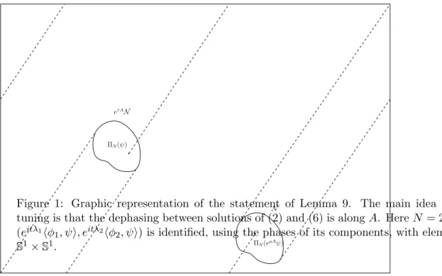
amount τ of time, as proved below (see Figure 1).
Lemma 9. Let ψ∈ H, µ > 0, N ∈ N, and N be a neighborhood of ΠN(eµAψ) in span{ϕ1, . . . , ϕN}.
Then there exists τ ≥ 0 such that eτ AN is a neighborhood of ΠNψ in span{ϕ1, . . . , ϕN}.
Proof. Without loss of generality we can assume thatN is an open ball B2ε(ΠN(eµAψ)) of radius 2ε
centered at ΠN(eµAψ), for some ε > 0.
Now, consider the sequence (βk)k∈N of sets
βk= Bε(ΠN(ekµAψ)).
All the elements of the sequence (βk)k∈N are of constant positive volume and are contained in the
common subset B∥ΠN(ψ)∥+ε(0) of span{ϕ1, . . . , ϕN}. Since the latter has finite volume, there exist two
integers ℓ, m ≥ 1 such that βℓ∩ βℓ+m ̸= ∅. Since e−ℓµA is an isomorphism of span{ϕ1, . . . , ϕN} we
deduce that
ΠN(ψ)
N eτ AN
ΠN(eµAψ)
Figure 1: Graphic representation of the statement of Lemma 9. The main idea underlying phase tuning is that the dephasing between solutions of (2) and (6) is along A. Here N = 2 and Π2(etAψ) = (eitλ1⟨ϕ
1, ψ⟩, eitλ2⟨ϕ2, ψ⟩) is identified, using the phases of its components, with elements of the torus S1× S1.
Therefore
ΠN(ψ)∈ B2ε(ΠN(emµAψ)) = e(m−1)µAB2ε(ΠN(eµAψ)) = e(m−1)µAN ,
which proves the lemma with τ = (m− 1)µ.
4.3 Final step
Proof of Theorem 2. Let ψ0 and ψ1 be in the unit sphere of H. For ε > 0 let n0∈ N be such that ψ0− Πn0ψ0 ∥Πn0ψ0∥ < ε3 and ψ1− Πn0ψ1 ∥Πn0ψ1∥ < ε3.
The Lie–Galerkin condition ensures the existence of n > n0 such that system (17) is controllable. By Proposition 8 there exist u∈ U, Tu ≥ 0, and γ ≥ 0 such that
Υu Tu ( Πn0ψ0 ∥Πn0ψ0∥ ) − eγA Πn0ψ1 ∥Πn0ψ1∥ < ε3.
By triangular inequality we have that ∥Υu Tu(ψ0)− eγAψ1∥ ≤ Υu Tu(ψ0)− ΥuTu ( Πn0ψ0 ∥Πn0ψ0∥ ) + ΥuTu ( Πn0ψ0 ∥Πn0ψ0∥ ) − eγA Πn0ψ1 ∥Πn0ψ1∥ + eγA Πn0ψ1 ∥Πn0ψ1∥ − eγAψ 1 = ψ0− Πn0ψ0 ∥Πn0ψ0∥ + ΥuTu ( Πn0ψ0 ∥Πn0ψ0∥ ) − eγA Πn0ψ1 ∥Πn0ψ1∥ + Πn0ψ1 ∥Πn0ψ1∥ − ψ1 < ε. Applying Lemma 9 there exists a time τ ≥ 0 such that eτ AΥu
Tu(ψ0) is ε-close to ψ1. The concate-nation of u and the zero function for a time τ then steers ψ0 into a ε- neighborhood of ψ1. Notice that such a concatenation is admissible since, in the case in whichU is the set of C∞ functions with values in U , the control u, given by Proposition 8, is zero with all derivatives at Tu.
5
Proof of Theorem 3
Theorem 3 states that under the Lie–Galerkin Control Condition it is possible to control approximately system (2) and, at the same time, to control it exactly in projection on a prescribed number of components. The first step in the proof consists in showing that the approximate controllability part is a consequence of the exact controllability in projections.
5.1 Exact controllability in projections implies approximate controllability
Lemma 10. Assume that for every n0 ∈ N, ψ1 ∈ H with ∥ψ1∥ = 1, and ψ2 ∈ H such that ∥ψ2∥ = 1
and ∥Πn0(ψ2)∥ < 1, there exist u ∈ U and T > 0 such that Πn0(Υ
u
T(ψ1)) = Πn0(ψ2). (19)
Then for every n ∈ N, ψin ∈ H with ∥ψin∥ = 1, and ψf ∈ H such that ∥ψf∥ = 1 and ∥Πn(ψf)∥ < 1,
and for every ε > 0, there exist u∈ U and T > 0 such that
Πn(ΥuT(ψin)) = Πn(ψf) and ∥ΥuT(ψin)− ψf∥ < ε.
Proof. Let n, ε, ψin, and ψf as above. If ψf ∈ H has an infinite number of non-zero components then it is sufficient to take n0 ≥ n such that ∥Πn0ψf− ψf∥ < ε/2 and apply (19) with ψ1= ψinand ψ2 = ψf. If, instead, there exists n0 ∈ N such that ⟨ϕn0, ψf⟩ ̸= 0 and ⟨ϕk, ψf⟩ = 0 for every k > n0 then note that n0 > n and consider ψ2 defined component-wise as
⟨ϕk, ψ2⟩ = ⟨ϕk, ψf⟩ if k = 1, . . . , n0− 1, √ 1− η2⟨ϕ n0, ψf⟩ if k = n0, η⟨ϕn0, ψf⟩ if k = n0+ 1, 0 if k > n0+ 1,
5.2 A useful topological tool
The following topological result is standard in degree theory. We provide its proof for completeness. Similar results used in the control literature are, for instance, [2, Lemma 7] and [18, Lemma 4.1].
Lemma 11. Let X ⊂ Rn be open and bounded and let F ∈ C(X, Rn) be a homeomorphism between
X and F (X). Assume that y0 is in F (X) and consider 0 < ε ≤ dist(y0, F (∂X)). If G ∈ C(X, Rn)
satisfies
max
x∈∂X|F (x) − G(x)| < ε
then y0 ∈ int(G(X)).
Proof. Consider the homotopy h ∈ C([0, 1] × ¯X,Rn) defined by h(t, x) = tF (x) + (1− t)G(x). By
definition of ε we have that h(t, x)̸= y0 for every t∈ [0, 1] and x ∈ ∂X. In particular the topological degree d(h(t,·), X, y0) is well defined for every t∈ [0, 1]. Since F |X is a homeomorphism and y0 ∈ F (X) then
d(F, X, y0)̸= 0 and by homotopy invariance
d(G, X, y0)̸= 0 which implies that y0∈ int(G(X)).
5.3 Normal controllability
In this section we consider ψ1 and ψ2 unit vectors in H and n0 ∈ N such that ∥Πn0(ψ2)∥ < 1. Let
n > n0 be such that the Lie–Galerkin Control Condition holds. Let now ˜ψ2 ∈ S2n−1 be such that Πn0(ψ2) = Πn0( ˜ψ2). By classical results of controllability (see [21] and [34, Theorem 4.3]) system (17) is normally controllable at ˜ψ2, in the sense that there exist M1, . . . , Mk∈ Wn and t1, . . . , tk> 0 such
that the map
E : (s1, . . . , sk)7→ eskMk ◦ · · · ◦ es1M1(ϕ1) has rank 2n− 1 at (t1, . . . , tk) and
E(t1, . . . , tk) = ˜ψ2.
Since n > n0 and ∥Πn0( ˜ψ2)∥ < 1, there exist j1, . . . , j2n0 ∈ {1, . . . , k} such that the map
F (sj1, . . . , sj2n0)7→ Πn0 (
E(t1, . . . , tj1−1, sj1, tj1+1, . . . , tj2n0−1, sj2n0, tj2n0+1, . . . , tk) )
has rank 2n0 at (tj1, . . . , tj2n0) and
F (tj1, . . . , tj2n0) = Πn0(ψ2) (
= Πn0( ˜ψ2) )
.
Now let ρ > 0 be such that
X := Bρ(tj1, . . . , tj2n0)⊂ (0, +∞)
2n0 and F is a diffeomorphism between X and F (X). Let
η = inf (s1,...,s2n0)∈∂X
∥F (s1, . . . , s2n0)− Πn0(ψ2)∥, (20)
Lemma 12. There exist γ ≥ 0 and a map associating with every (s1, . . . , s2n0)∈ ¯X a control v
s∈ U
and Ts > 0 such that the image of the mapping
G : X¯ → span{ϕ1, . . . , ϕn0} (s1, . . . , s2n0) 7→ Πn0 ( ΥvTss(ψ1) ) contains Πn0(e γAψ 2) in its interior.
Proof. Let η be as in (20). By Theorem 2 there exists w∈ U steering ψ1, η/2-close to ϕ1. Applying Proposition 8 with
(τ1, . . . , τk) = (t1, . . . , tj1−1, sj1, tj1+1, . . . , tj2n0−1, sj2n0, tj2n0+1, . . . , tk),
we deduce the existence of a family of controls us, depending continuously on s∈ X such that max s∈ ¯X ∥F (s) − e −γAΠ n0 ( ΥuTs usϕ1 ) ∥ < η/2.
Define vs as the concatenation of w and us. The continuity of G with respect to s is ensured by Assumption (A5). The conclusion then follows from Lemma 11.
5.4 Final step
We are now ready to conclude the proof of Theorem 3.
Proof of Theorem 3. By Lemma 10 it enough to prove that for every n0 ∈ N, ψ1∈ H with ∥ψ1∥ = 1, and ψ2 ∈ H such that ∥ψ2∥ = 1 and ∥Πn0(ψ2)∥ < 1, there exist u ∈ U and T > 0 such that
Πn0(Υ
u
T(ψ1)) = Πn0(ψ2).
Lemma 12 guarantees the existence of a neighborhood N ⊂ G(X) of Πn0(e
γAψ
2). By Lemma 9 with µ = γ, there exists τ ≥ 0 and ζ ∈ N such that eτζ = Πn0(ψ2). Let s ∈ X be such that Πn0
(
ΥvTss(ψ1) )
= ζ. The concatenation of vs and the zero function for a time τ then steers ψ1 to some ψ3 such that Πn0ψ3 = Πn0ψ2. Notice that such a concatenation is admissible since, in the case in whichU is the set of C∞ functions with values in U , the control vs, given by Lemma 12 (see also Proposition 8), is zero with all derivatives at Ts.
References
[1] R. Adami and U. Boscain. Controllability of the Schr¨odinger equation via intersection of eigen-values. In Proceedings of the 44th IEEE Conference on Decision and Control, pages 1080–1085, 2005.
[2] A. A. Agrachev and M. Caponigro. Dynamics control by a time-varying feedback. J. Dyn. Control
Syst., 16(2):149–162, 2010.
[3] A. A. Agrachev and Y. L. Sachkov. Control theory from the geometric viewpoint, volume 87 of Encyclopaedia of Mathematical Sciences. Springer-Verlag, Berlin, 2004. Control Theory and Optimization, II.
[4] J. M. Ball, J. E. Marsden, and M. Slemrod. Controllability for distributed bilinear systems. SIAM
J. Control Optim., 20(4):575–597, 1982.
[5] K. Beauchard and J.-M. Coron. Controllability of a quantum particle in a moving potential well.
J. Funct. Anal., 232(2):328–389, 2006.
[6] K. Beauchard and C. Laurent. Local controllability of 1D linear and nonlinear Schr¨odinger equations with bilinear control. J. Math. Pures Appl., 94(5):520–554, 2010.
[7] R. S. Bliss and D. Burgarth. Quantum control of infinite-dimensional many-body systems. Phys.
Rev. A, 89:032309, Mar 2014.
[8] A. M. Bloch, R. W. Brockett, and C. Rangan. Finite controllability of infinite-dimensional quantum systems. IEEE Trans. Automat. Control, 55(8):1797–1805, 2010.
[9] U. Boscain, M. Caponigro, T. Chambrion, and M. Sigalotti. A weak spectral condition for the controllability of the bilinear schr¨odinger equation with application to the control of a rotating planar molecule. Communications in Mathematical Physics, 311(2):423–455, 2012.
[10] U. Boscain, M. Caponigro, and M. Sigalotti. Multi-input Schr¨odinger equation: Controllability, tracking, and application to the quantum angular momentum. Journal of Differential Equations, 256(11):3524 – 3551, 2014.
[11] U. Boscain, F. Chittaro, P. Mason, and M. Sigalotti. Adiabatic control of the Schroedinger equation via conical intersections of the eigenvalues. IEEE Trans. Automat. Control, 57(8):1970– 1983, 2012.
[12] N. Boussa¨ıd, M. Caponigro, and T. Chambrion. Regular propagators of bilinear quantum systems. Preprint arXiv:1406.7847, 2016.
[13] T. Chambrion. Periodic excitations of bilinear quantum systems. Automatica J. IFAC,
48(9):2040–2046, 2012.
[14] T. Chambrion, P. Mason, M. Sigalotti, and U. Boscain. Controllability of the discrete-spectrum Schr¨odinger equation driven by an external field. Ann. Inst. H. Poincar´e Anal. Non Lin´eaire,
26(1):329–349, 2009.
[15] D. D’Alessandro. Introduction to quantum control and dynamics. Applied Mathematics and Nonlinear Science Series. Boca Raton, FL: Chapman, Hall/CRC., 2008.
[16] R. El Assoudi, J. P. Gauthier, and I. A. K. Kupka. On subsemigroups of semisimple Lie groups.
Ann. Inst. H. Poincar´e Anal. Non Lin´eaire, 13(1):117–133, 1996.
[17] J.-P. Gauthier and G. Bornard. Controlabilit´e des syst`emes bilin´eaires. SIAM J. Control Optim., 20(3):377–384, 1982.
[18] O. Glass and L. Rosier. On the control of the motion of a boat. Math. Models Methods Appl.
Sci., 23(4):617–670, 2013.
[19] M. Herrero-Collantes and J. C. Garcia-Escartin. Quantum random number generators. Rev. Mod.
[20] V. Jurdjevic and I. Kupka. Control systems on semisimple Lie groups and their homogeneous spaces. Ann. Inst. Fourier (Grenoble), 31(4):vi, 151–179, 1981.
[21] V. Jurdjevic and H. J. Sussmann. Control systems on Lie groups. J. Differential Equations, 12:313–329, 1972.
[22] M. Keyl, R. Zeier, and T. Schulte-Herbrueggen. Controlling Several Atoms in a Cavity. New J.
Phys., 16:065010, 2014.
[23] X. Ma, X. Yuan, Z. Cao, B. Qi, and Z. Zhang. Quantum random number generation. npj Quantum
Information, 2:16021, 2016.
[24] P. Mason and M. Sigalotti. Generic controllability properties for the bilinear Schr¨odinger equation.
Comm. Partial Differential Equations, 35(4):685–706, 2010.
[25] M. Mirrahimi. Lyapunov control of a quantum particle in a decaying potential. Ann. Inst. H.
Poincar´e Anal. Non Lin´eaire, 26(5):1743–1765, 2009.
[26] M. Mirrahimi and P. Rouchon. Controllability of quantum harmonic oscillators. IEEE
Transac-tions on Automatic Control, 49(5):745–747, 2004.
[27] M. Morancey and V. Nersesyan. Simultaneous global exact controllability of an arbitrary number of 1D bilinear Schr¨odinger equations. J. Math. Pures Appl. (9), 103(1):228–254, 2015.
[28] V. Nersesyan. Growth of Sobolev norms and controllability of the Schr¨odinger equation. Comm.
Math. Phys., 290(1):371–387, 2009.
[29] V. Nersesyan. Global approximate controllability for Schr¨odinger equation in higher Sobolev norms and applications. Ann. Inst. H. Poincar´e Anal. Non Lin´eaire, 27(3):901–915, 2010.
[30] V. Nersesyan and H. Nersisyan. Global exact controllability in infinite time of Schr¨odinger equa-tion. J. Math. Pures Appl. (9), 97(4):295–317, 2012.
[31] E. Paduro and M. Sigalotti. Approximate controllability of the two trapped ions system. Quantum
Inf. Process., 14(7):2397–2418, 2015.
[32] M. Reed and B. Simon. II: Fourier Analysis, Self-Adjointness, volume 2. Elsevier, 1975.
[33] S. G. Schirmer, H. Fu, and A. I. Solomon. Complete controllability of quantum systems. Physical
Review A, 63(6):063410, 2001.
[34] H. J. Sussmann. Some properties of vector field systems that are not altered by small perturba-tions. J. Differential Equations, 20(2):292–315, 1976.
[35] G. Turinici. On the controllability of bilinear quantum systems. In M. Defranceschi and C. Le Bris, editors, Mathematical models and methods for ab initio Quantum Chemistry, volume 74 of Lecture