and technological progress in the automobile sector
The MIT Faculty has made this article openly available.
Please share
how this access benefits you. Your story matters.
Citation
Knittel, Christopher R. “Automobiles on Steroids: Product Attribute
Trade-Offs and Technological Progress in the Automobile Sector.”
American Economic Review 101.7 (2011): 3368–3399. Web.
As Published
http://dx.doi.org/10.1257/aer.101.7.3368
Publisher
American Economic Association
Version
Final published version
Citable link
http://hdl.handle.net/1721.1/75250
Terms of Use
Article is made available in accordance with the publisher's
policy and may be subject to US copyright law. Please refer to the
publisher's site for terms of use.
3368
The transportation sector accounts for over 30 percent of US greenhouse gas emissions. Despite this, the United States has done little over the past 25 years to incentivize increases in passenger automobile fuel economy. Corporate Average Fuel Economy (CAFE) standards for passenger cars have not increased since 1990. For light trucks and SUVs, they have grown by only 10 percent since 1990. CAFE standards increased substantially for passenger vehicles from 1978 to 1990, but the shift from passenger cars to light trucks and SUVs meant the sales-weighted CAFE standard has changed little since 1983. In contrast to European policymakers, US policymakers have also been reluctant to incentivize carbon reductions through either gasoline or carbon taxes. This, coupled with lower oil prices, led to a 30 per-cent reduction in real gasoline prices from 1980 to 2004. While rapid increases in gas prices appear to have led to a shift to fuel economy from 2006 to 2008, gasoline prices did not include the externality costs of climate change and other externalities.1
1 See Meghan Busse, Knittel, and Florian Zettelmeyer (2009) for a detailed study of how gas prices affected fuel economy. These changes are also evident in the aggregate data. New car fleet fuel economy increased by roughly 10 percent from 2004 to 2008, a period where gasoline prices increased by over 70 percent.
Automobiles on Steroids: Product Attribute Trade-Offs and
Technological Progress in the Automobile Sector
†By Christopher R. Knittel*
This paper estimates the technological progress that has occurred since 1980 in the automobile industry and the trade-offs faced when choosing between fuel economy, weight, and engine power charac-teristics. The results suggest that if weight, horsepower, and torque were held at their 1980 levels, fuel economy could have increased by nearly 60 percent from 1980 to 2006. Once technological prog-ress is considered, meeting the Corporate Average Fuel Economy
(CAFE) standards adopted in 2007 will require halting the trend
in weight and engine power characteristics, but little more. In con-trast, the standards recently announced by the new administration, while attainable, require nontrivial “downsizing.” (JEL L50, L60)
* Sloan School of Management, Massachusetts Institute of Technology, 100 Main Street, Cambridge, MA 02142, and NBER (email: [email protected]). This paper has benefitted from conversations with Severin Borenstein, K. G. Duleep, David Greene, Jonathan Hughes, Mark Jacobsen, Doug Miller, David Rapson, Ken Small, Anson Soderbery, Dan Sperling, Nathan Wilmot, Frank Wolak, and Catherine Wolfram, as well as seminar participants at Stanford, MIT, UC Davis, and the UC Energy Institute. Tom Blake, Omid Rouhani, and Anson Soderbery pro-vided excellent research assistance. Financial support from the California Air Resource Board and the Institute of Transportation Studies at UC Davis is gratefully acknowledged. I am grateful to K. G. Duleep for providing me with data.
† To view additional materials, visit the article page at http://www.aeaweb.org/articles.php?doi=10.1257/aer.101.7.3368.
The lack of either pricing mechanisms or standards has meant US fleet fuel econ-omy has been stagnant despite apparent technological advances. From 1980 to 2004 the average fuel economy of the US new passenger automobile fleet increased by less than 6.5 percent. During this time, the average horsepower of new passenger cars increased by 80 percent, while the average curb weight increased by 12 percent. Changes in light-duty trucks have been even more pronounced. Average horsepower increased by 99 percent and average weight increased by 26 percent from 1984 to 2004. In addition, the change within passenger cars and light trucks hides much of the story. In 1980 light truck sales were roughly 20 percent of total passenger vehicles sales; in 2004, they were over 51 percent.
These changes in vehicle characteristics are driven by consumer preferences and shifts in the weight/power/fuel economy iso-cost function. A large literature focuses on estimating consumer preferences for fuel economy and power charac-teristics measured as either horsepower, torque, or acceleration.2 The goal of this paper is to better understand the technological trade-offs that manufacturers and consumers face when choosing between fuel economy, weight, and engine power characteristics, as well as how this relationship has changed over time. The results serve as a guide as to how the market may respond to increases in CAFE standards or a carbon tax, as well as how far regulatory standards can push fleet fuel economy.
Using detailed model-level data from 1980 to 2006, I answer two related ques-tions. One, how would fuel economy today compare to fuel economy in 1980 if we had held size and power constant? And two, how would new fleet fuel economy look in the future if we were to continue to progress at rates observed in the data?
The results suggest that if weight, horsepower, and torque were held at their 1980 levels, fuel economy for both passenger cars and light trucks could have increased by nearly 60 percent from 1980 to 2006. This is in stark contrast to the 15 percent by which fuel economy actually increased. Technological progress was most rapid during the early 1980s, a period where CAFE standards were rapidly increasing and gasoline prices were high. This is consistent with the results of Richard G. Newell, Adam B. Jaffe, and Robert N. Stavins (1999) and David Popp (2002) which find that the rate of energy efficiency innovation depends on both energy prices (Newell, Jaffe, and Stavins; Popp) and regulatory standards (Newel, Jaffe, and Stavins).
The estimated trade-off between weight and fuel economy suggests that, for pas-senger cars, fuel economy increases by over 4 percent for every 10 percent reduction in weight. On average, fuel economy increases by 2.7 percent for every 10 percent reduction in horsepower. The effect of torque is less precisely estimated. For light -duty trucks, weight reductions of 10 percent are associated with increases in fuel economy of 3.6 percent, and a 10 percent increase in torque is correlated with a 3 percent increase in fuel economy. The association with horsepower is not pre-cisely estimated.
The results shed light on the changes in vehicle attributes and rates of technologi-cal progress required to meet the CAFE standards recently adopted by both the Bush and Obama administrations. The Bush CAFE standards call for an economy-wide
2 For example, see such seminal papers as Pinelopi K. Goldberg (1995) and Steven Berry, James Levinsohn, and Ariel Pakes (1995). Typically, the influence of gasoline prices is not the focus of these papers. Two exceptions are Thomas Klier and Joshua Linn (2009) and James W. Sawhill (2008).
average fuel efficiency of 35 MPG by 2020; the Obama standards call for an aver-age fuel economy of 35.5 MPG by 2016. I use the estimates above to calculate new fleet fuel economy in 2020 and 2016 varying: (i) the rate of technological progress; (ii) average vehicle weight and engine power; and (iii) the passenger car–to–light truck ratio. I find that meeting the Bush standards will not require large behavioral changes, but will require halting the rate of growth in engine power and weight. In particular, if we continue with the average estimated rate of technological progress and current car/truck mix, the standard can be met by reversing the increase in weight and engine power that has occurred since 1980 by less than 25 percent.3 Alternatively, shifting the car-to-truck ratio back to levels observed in the 1980s will exceed the standard by roughly 2 MPG. The results also suggest that reducing weight and engine power characteristics to their 1980 levels combined with rates of technological progress that were typical during the increases in CAFE standards in the early 1980s lead to fleet fuel economy over 52 MPG by 2020.
Meeting the Obama standards will require “downsizing” of fleet attributes, although the standards are certainly attainable. With average rates of technologi-cal progress, new vehicle fleet fuel economy can reach 35.5 MPG by shifting the car/truck mix to their 1980 levels while at the same time reversing the weight and power characteristic gains since 1980 by 25 percent. Alternatively, the car/truck mix can remain constant, but weight and power be reduced by roughly 50 percent of the gains since 1980. A mixture of these two extremes is also possible. With rapid technological progress, along with aggressive shifts in the car/truck mix and down-sizing, fleet fuel economy can reach over 47 MPG by 2016.
To be clear, these results do not speak to the social welfare implications of the two CAFE standards or predict equilibria. Rather, the results uncover how fleet fuel economy varies car/truck mixtures and changes in power and weight char-acteristics for given levels of technological progress. Viewed in this way, these calculations complement work by Goldberg (1998) which estimates the effects of CAFE standards on equilibrium outcomes in the short run, i.e., when vehicle attri-butes and technology are fixed. Therefore, in her paper CAFE compliance relies on pricing strategies that shift the relative quantities of existing vehicles.
The remainder of the paper is organized as follows. Section I discusses the theo-retical and empirical models. In Section II, I discuss the sources of technological progress in the automobile industry. Section III discusses the data. Section IV pro-vides graphical evidence of both trade-offs and technological progress. In Section V, I discuss the empirical results, including estimated trade-offs, technological prog-ress, and compliance strategies for the new CAFE standards. Section VI estimates alternative models and investigates robustness. In Section VII, I provide evidence that the results are not driven by either within-year or cross-year changes in how much manufacturers spend on engine technology. Finally, Section VIII concludes the paper.
3 If we infer causality for the trade-offs above, this can be met by either altering the makeup of existing vehicles or shifting which vehicles are purchased. If the trade-offs are viewed as simply correlations, then this represents shifting which vehicles, among those vehicles that are already offered, are purchased.
I. Theoretical and Empirical Models
Underlying the empirical work is a marginal cost function for producing a vehicle at time t with a given level of fuel economy, mp git , horsepower, h pit , torque, t qit ,
other attributes related to fuel economy, Xit , and attributes related to other aspects of the vehicle, Zit . I represent this as
(1) cit = C(mp g it , w it , h pit, t q it , X it , Z it , t).
One method for estimating technological progress is to estimate how this function has changed over time. This is difficult for two reasons. First, the dimension of the Zit vec-tor required to adequately control for changes in vehicle attributes across other dimen-sions is large. Second, marginal cost data are not available. An obvious proxy is price data; however, given the numerous changes in the industrial structure of the auto indus-try a concern is that estimates of technological progress would also capture changes in mark-ups over time. Instead, I focus on the level sets of the marginal cost function.
I assume that the marginal cost function is additively separable in (mp g it , w it , h pit ,
tit , X it) and Z it , yielding
(2) cit = C 1(mp g it , w it , h pit, t q it , X it , t) + C 2( Z it , t).
The C 2 function captures components of the marginal cost function that are unre-lated to fuel economy, such as interior quality, options like air-conditioning (which do not affect the EPA fuel economy rating), etc. The level sets of C 1 are given as (3) mp git = f ( w it , h pit , t it , X it , t | C 1 = σ).
Technological progress is modeled as “input” neutral in the sense that it is multipli-cative to the function relating fuel economy with power and weight, yielding4 (4) mp git = T t f ( w it , h pit , t it , X it , ∈ it | C 1 = σ).
A. Additional Factors
Consistent estimation of the level sets and how they have changed over time due to technological progress requires that the value of C 1 does not vary over time or within year. Stated differently, the value of C 1 is in the error term in the empirical specification. Omitting expenditures on technology from the empirical model may lead to two sources of bias. First, if the goal is to estimate how the level sets have changed over time, holding how much is devoted to technology constant, then the estimated shifts in the level sets will be biased. The direction of the bias is unknown. If firms have increased the amount spent on these technologies over time, then the shifts will reflect both technological progress and this increase. In contrast, if firms have reduced expenditures on technology over time, the shifts will understate
technological progress. The second source of bias may come from within-year vari-ation in the cost devoted to technologies, if this varivari-ation is correlated with one of the characteristics. This would bias the estimates of the engineering relationship between fuel economy and engine power or weight.
Section VII provides detailed evidence that these biases are likely small by includ-ing a number of proxies for technological expenditures in the empirical models. I also note that, for much of the analysis, assuming shifts in the level sets reflect only technological progress is not required. Specifically, I use the estimates to answer two related questions. One, how would fuel economy today compare to fuel economy in 1980 if we had held size and power constant? And two, how would new fleet fuel economy look in the future if we were to continue to progress at rates observed in the data? Insofar as the observed increase in fuel economy captures both shifts in the level sets due to technological progress and increases in how much firms are devot-ing to technology, the results should be interpreted in this light. That is, the estimates should be interpreted as how fleet fuel economy in 2006, or some point in the future, would have changed if we had kept vehicle characteristics the same and continued with the observed changes in both the level sets and technology expenditures.
Besides the cost devoted to technologies, other factors alter the relationship between fuel economy, engine power, and weight. For example, vehicles with man-ual transmissions are able to achieve higher fuel economy than automatic transmis-sions, conditional on weight and engine power. Turbochargers also increase fuel efficiency. Insofar as my data allow, I control for a number of these factors, labelled as Xit . I discuss these variables below.
B. Empirical specification
To estimate the level sets I begin by making functional form assumptions for f (∙), while technological progress is modeled nonparametrically as a set of year fixed effects. I begin the analysis by focusing on two functional forms: Cobb-Douglas and translog. Section VI relaxes both of these assumptions. A mean zero error term, ϵ it ,
captures additional characteristics of the vehicle that are assumed to be uncorrelated with the other right-hand-side variables.
Under the Cobb-Douglas and translog assumptions, fuel economy is modeled, respectively, as5 (5) ln mp g* it = T t + β 1 ln wit + β 2 ln h pit + β 3 ln t qit + X it B + ϵ ′ it and (6) ln mp g it* = T t + β 1 ln wit + β 2 ln h pit + β 3 ln t qit + γ 1(ln w it ) 2 + γ 2(ln h p it ) 2 + γ 3(ln t q it ) 2 + δ 1 ln wit ln h pit + δ 2 ln wit ln t qit + δ 3 ln h pit ln tit + X it′ B + ϵ it .6
5 Fuel economy is often represented as gallons per mile. By taking the log of miles per gallon, the empirical model is equivalent to measuring fuel economy in terms of gallons per mile.
6 One might be concerned that weight and power are endogenous, in the sense that they are correlated with unobserved vehicle-level productivity. For a discussion, see, for example, G. Steven Olley and Pakes (1996). Many
II. Sources of the Shifts
Technological progress represents not only increases in engine technology, but also advances in transmissions, aerodynamics, rolling resistance, etc. Since the early 1980s, a number of fuel economy/power technologies have become prevalent in vehicles. On the engine side, large efficiency gains from replacing carburetors with fuel injection have been realized. In contrast to an engine in the 1980s, the typical engine today has the camshaft—the apparatus that lifts the valves as it rotates— above the engine head. This eliminates friction causing pushrods and rocker arms. In addition, the majority of engines today have multiple camshafts, allowing for more than two valves per cylinder; many also have variable valve timing technolo-gies. More valves allow for the smoother flow of both the fuel/air mixture and exhaust in and out of the cylinder, while variable valve timing allows for the timing of the valve lift to adjust to driving conditions.7 Turbochargers or superchargers also increase the efficiency of an engine by using a turbine, spun by either the engine’s exhaust (turbocharger) or the rotation of the engine’s crankshaft (supercharger), to force air into the engine. This allows for a smaller displacement while holding horsepower constant.8 Most recently, cylinder deactivation and hybrid technology are becoming more prevalent. Hybrid technologies use both a gasoline engine and electric motor (with a battery) to propel the vehicle. When there is sufficient stored electricity, the car runs solely on the electric motor or both the engine and electric motor. During times when the vehicle is coasting, the electric motor runs in reverse, thereby recharging the battery. Cylinder deactivation opens the valves on a set of cylinders during times when less power is needed, thus not using these cylinders to power the automobile.
Transmissions have also become more efficient by utilizing more speeds, vari-able speed transmissions, and torque converter lock-up. Increasing the number of speeds allows the engine to operate at more efficient revolutions per minute (RPMs). Variable speed transmissions have a continuous number of speeds allow-ing the engine’s RPMs to remain relatively constant. Torque converter lock-ups reduce the efficiency losses by fixing the torque converter to the drivetrain at high-way speeds. Improvements to other portions of the drivetrain include an increased use of front-wheel drive which increases fuel efficiency by having the engine closer to the wheels receiving power and by often having the engine turned 90 degrees so that the rotation of the engine mirrors the rotation of the wheels. Finally, advanced materials, tire improvements, and advances in aerodynamics and lubricants have also lead to efficiency improvements.
of the empirical models include fixed manufacturer effects which capture unobserved productivity that is constant across manufacturers, leaving only within-manufacturer differences in productivity across models in the error term. I treat weight and power as exogenous to this component of unobserved productivity, thus following the existing empirical literature that estimates automobile marginal cost as a function of vehicle characteristics (e.g., Berry, Levinsohn, and Pakes 1995; Goldberg 1995, 1998). I note that the estimated trade-offs and technological progress change little when manufacturer fixed effects are included, suggesting that any additional endogeneity concerns are likely to be small.
7 D. M. Chon and J. B. Heywood (2000) find that multiple valves increase fuel efficiency 2 to 5 percent above two-valve designs, while variable valve timing increases fuel efficiency by roughly 2 to 3 percent.
8 Hermann Josef Ecker, Dave Gill, and Markus Schwaderlapp (2000) find that supercharging diesel engines can yield fuel efficiency improvements as large as 10 percent when combined with variable valve timing.
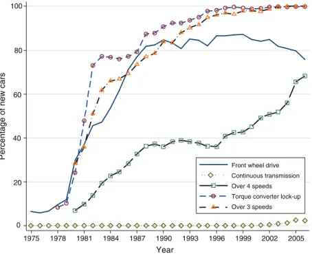
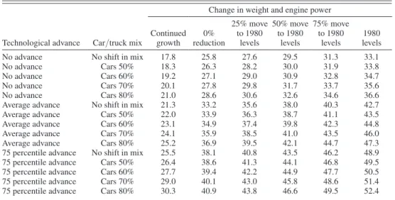
The penetration of a number of these technologies since 1975 is plotted in Figures 1 and 2.9 Figure 1 focuses on engine-related technologies, while Figure 2 focuses on other parts of the drivetrain. Figure 1 illustrates that, compared to the typical vehicle built in 1980, a vehicle today is more likely to be fuel injected, have more than two valves per cylinder, and have variable valve timing.10 While turbochargers and super-chargers have not penetrated the market nearly as much as these other technologies, their use has also increased. Hybrid technologies have also increased in recent years. The diffusion of nonengine drivetrain technologies has also been rapid. Front-wheel drive, torque converter lock-ups (for vehicles with an automatic transmission), and transmissions with at least four gears became commonplace in the early 1980s and essentially standard by 1990. By 2006, nearly 70 percent of vehicles had a transmis-sion with at least five speeds; continuous transmistransmis-sions have also entered the market.
A number of technologies are also “waiting in the wings.” These include advances in hybrid technology, plug-in hybrids, camless engines, further reductions in engine friction, higher voltage electrical systems, and improved air conditioning.11
9 Data from all variables, other than transmission speeds, are taken from http://www.epa.gov/otaq/fetrends.htm. Data for transmission speeds are taken from the model-level data used in this paper.
10 Daniel Snow (2009) finds that the improvements to fuel economy from increased penetration in fuel injection were larger than this graph may suggest for two reasons. First, there was positive selection in the sense that fuel injection was first used in applications that led to the largest efficiency gains. Second, some of the benefits from fuel injection technology spilled over to carburetors making the older technology more efficient.
11 For a discussion of the cost of these potential technologies and their impacts on fuel economy, see, for example, David L. Greene and K. G. Duleep (1993); John DeCicco and Marc Ross (1996); and DeCicco, Feng An, and Ross (2001).
0 20 40 60 80 100
Percentage of new cars
1975 1978 1981 1984 1987 1990 1993 1996 1999 2002 2005
Year
Fuel injection Variable valve timing Turbo/supercharger Multiple valves Hybrid
Figure 1. Penetration of Engine-Related Technologies that Would Shift the Production Possibilities Frontier
III. Data
I use model-level data on nearly all vehicles sold within the United States and subject to CAFE standards. Therefore, the analysis omits vehicles that have a gross vehicle weight in excess of 8,500 pounds, which are exempt from CAFE regulation. The results should be interpreted in this light, reflecting the progress and trade-offs associated with vehicles with curb weights below 8,500 pounds. Fuel economy data come from the National Highway Traffic Safety Administration (NHTSA) and are supplemented with data from Automobile news and manufacturer websites. The data report the weighted average of city and freeway fuel economy, weight, maxi-mum horsepower, and maximaxi-mum torque.12 The weight measures for cars and trucks differ. For passengers cars, the data report the curb weight—the weight of the vehi-cle unloaded. For light-duty trucks the weight measure is the vehivehi-cle “test weight,” which is more discrete than the curb weight. In addition, data are available on fuel type, aspiration type (e.g., turbocharger), transmission type, and engine size.13
12 Fuel economy is measured as a weighted average of city fuel economy (55 percent) and highway fuel econ-omy (45 percent) from the unadjusted measures (i.e., not the fuel economy measures on the labels). Horsepower and torque are closely related. In fact, at a given RPM, horsepower = torque × RPM/5,250. Because the maximum values used in the analysis occur at different RPM levels, there is still information in each. The results are robust to including only one of the two measures.
13 I take a few steps to uncover errors in the data. Specifically, I exclude all vehicles that have missing observa-tions and observaobserva-tions with torque exceeding 2,000 ft. lbs. This omits 5.1 percent of the sample; 97 percent of these are due to missing data. From looking at the data, it appears as though the RPM level at the maximum torque level and torque are reversed for some of these observations. As a frame of reference, the 2006 Dodge Viper has a
0 20 40 60 80 100
Percentage of new cars
1975 1978 1981 1984 1987 1990 1993 1996 1999 2002 2005
Year
Front wheel drive Continuous transmission Over 4 speeds Torque converter lock-up Over 3 speeds
Figure 2. Penetration of Nonengine-Related Technologies that Would Shift the Production Possibilities Frontier
Whether to include these additional covariates depends on the question of inter-est. If one were interested in understanding how much more efficient a normally aspirated, gasoline passenger car with an automatic transmission, conditional on its weight, horsepower, and torque, is today compared to in 1980, we would want to include not only weight, horsepower, and torque, but also all of the additional variables. If, instead, one were interested in knowing how much more efficient is a vehicle today, compared to in 1980, allowing for changes in engine size, aspiration-rates, fuel types, etc., then the additional variables should be omitted. That is, if a portion of technological advancement is coming from advances in turbo equipment, fuel shifting, or the ability to extract more power from smaller engines, we would not want to include the other covariates, thereby allowing the year effects to absorb these advances. It seems fairly clear that one would not want to condition on engine size; the other variables are not so clear. In what follows, I present results including all of the variables and results including only transmission and fuel type. They are broadly consistent with each other, but, as expected, omitting the other variables tends to imply slightly larger technological advances. In addition, Figure 2 suggests that over the sample period the efficiency gap between of manual and automatic transmissions has shrunk. To account for this, I interact the manual transmission indicatory variable with a time trend.14
Finally, a number of the empirical models include manufacturer fixed effects. Given the variety of ownership changes over the sample, I take steps to construct a stable definition of manufacturers. For example, I keep Mercedes and Chrysler separate throughout the sample.
IV. Summary Statistics and Graphical Evidence
Before estimating econometric models of the level sets, I provide summary statis-tics and graphical analyses of both the trade-offs and shifts.
Table 1 reports the summary statistics for vehicles across the entire sample, and separately for 1980 and 2006. It is important to note that these statistics represent what cars were available; they differ from the new vehicle fleet summary statistics since the fleet summary statistics are obviously sales weighted. The average fuel economy for passenger cars is just under 28 MPG for the entire sample. The least fuel efficient vehicle has a fuel economy of 8.7 MPG (the 1990 Lamborghini Countach), while the most fuel efficient vehicle is the 2000 Honda Insight at 76.4 MPG.15 The average fuel economy of automobiles offered was over 27 MPG in 2006, while it was under 23 MPG in 1980. This represents an increase of roughly 18.5 percent.
The average car has a curb weight of over 3,000 pounds. Weight has increased by nearly 14 percent over the sample. Remarkably, horsepower has more than doubled over this time, while torque has increased by over 45 percent. All of these gains have occurred with smaller engines. Fewer diesel engines are offered now, compared
maximum torque of 712 ft. lbs.; the Lamborghini Diablo has 620 ft. lbs. of torque. I also omit observations with fuel economy below 5 MPG and observation with fuel economy above 70 MPG (except for the Honda Insight).
14 A squared term for time was also tried, but was not statistically significant. Time trends interacted with the other indicator variables were also not statistically significant.
15 The results of Section V are robust to excluding the “exotic” manufacturers, such as Lamborghini, Ferrari, etc., as these make up very few observations in the data.
to in 1980, while the percentage of turbocharged and supercharged vehicles has increased. A similar number of manual transmissions are offered in the two peri-ods. Acceleration has increased by nearly 40 percent over this time period.16 These changes are similar to changes in the new passenger car fleet from 1980 to 2004 (thus, sales weighted). For the fleet, fuel economy increased by 19.8 percent, weight increased by 13 percent, and horsepower increased by 80 percent. Diesel penetra-tion went from 4.2 percent to 0.3 percent, due in large part to increasing limits on particulate matter emissions. The percentage of cars with either a turbocharger or supercharger increased from 1.0 percent to 5.9 percent, and the percentage of vehi-cles with manual transmissions went from 30 percent to 20 percent.
Among vehicles that were offered, the increases in fuel economy for light-duty trucks was 35 percent. Weight gains have been similar to passenger vehicles. Horsepower increased by 70 percent and torque by 15 percent. Acceleration has not increased as much as with passenger cars, but has still increased by over 25 percent. Fleet data are available for light-duty trucks for fuel economy from 1980 to 2004 and for other attributes from 1984 to 2004. For the actual fleet, over these time periods, fuel economy increased by 15.7 percent, weight increased by 26 percent, horsepower increased by 99 percent, diesel penetration went from 2.8 percent to 2.5 percent, the percent of cars with either a turbocharger or supercharger increased
16 Acceleration is imputed using the EPA Light-Duty Automotive Technology and Fuel Trends: 1975 to 2007 estimate for acceleration of t = F(HP/WT ) −f with F and f: 0.892 and 0.805 for automatic transmissions and 0.967 and 0.775 for manual transmissions. Because the analysis uses the natural log of each variable, acceleration is implicitly controlled for.
Table 1—Summary Statistics
Variable Mean SD Min Max Mean in 1980 Mean in 2006
Passenger cars Fuel economy 27.90 6.43 8.70 76.40 22.89 27.11 Curb weight 3,019.45 593.70 1,450.00 6,200.00 3,041.64 3,455.04 HP 157.14 76.97 48.00 660.00 110.63 247.02 Torque 238.71 105.16 69.40 1,001.00 226.29 329.67 Acceleration 10.56 2.52 3.03 20.75 13.14 8.08 Liters 2.77 1.15 1.00 8.30 3.41 3.22 Diesel 0.03 0.18 0 1 0.07 0.01 Manual 0.38 0.49 0 1 0.35 0.35 Supercharged 0.01 0.11 0 1 0.00 0.05 Turbocharged 0.11 0.31 0 1 0.03 0.15 Sample size 14,337 507 572 Light trucks Fuel economy 20.76 4.65 9.90 45.10 16.81 22.80 Curb weight 3,898.45 778.25 1,920.00 6,700.00 3,877.33 4,427.68 HP 160.37 53.76 48.00 500.00 138.59 236.52 Torque 296.01 90.95 76.60 750.00 304.48 351.21 Acceleration 12.13 2.34 4.89 28.19 13.16 9.65 Liters 4.06 1.33 1.20 8.30 4.72 3.95 Diesel 0.05 0.21 0 1 0.02 0.00 Manual 0.33 0.47 0 1 0.42 0.17 Supercharged 0.00 0.05 0 1 0.00 0.01 Turbocharged 0.01 0.11 0 1 0.00 0.03 Sample size 12,805 669 470
from 0.4 percent to 1.5 percent, and the percentage of manual transmissions went from 41.8 percent to 7.0 percent.
Figures 3 through 6 provide graphical evidence of the trade-offs that exist between fuel economy and other automobile attributes and the technological progress that took place from 1980 to 2006. Figure 3 plots fuel economy against weight separately for 1980 and 2006 for passenger cars. For visual ease, I truncate fuel economy above 50 MPG. A lowess smoothed nonparametric line is also fit-ted through the data. The figure suggests that a 3,000 pound passenger car gets roughly 10 more MPG in 2006, compared to 1980. This increase is roughly con-stant over the weight distributions. At the mean fuel economy level in 1980, this reflects a 45 percent increase. Similarly, Figure 4 suggests that a passenger car with 150 horsepower gets roughly 12 more MPG in 2006 than in 1980. As with weight the shift in the iso-cost curve is fairly parallel. The graph of fuel economy versus torque mirrors this.
To confirm that similar trade-offs exist for light-duty trucks, Figures 5 and 6 repeat the exercise. Two things are worth noting. First, the magnitude of the shift is similar to passenger cars. Second, the shift is not as constant across the attributes when compared with passenger cars. These figures motivate the econometric mod-els, which allows for nonparallel shifts.
V. Econometric Results
Tables 2 and 3 report the level set estimates for passenger cars. Tables 4 and 5 report the results for light trucks.17 For brevity, I omit the standard errors
17 These results do not weight by sales. If technological constraints are the same across firms and vehicle classes (within cars and trucks), there is little reason to weight by sales. If, however, the production frontiers dif-fer, then estimates weighting vehicles by sales might be preferred. The online Appendix reports results where the
Figure 3. Fuel Economy versus Weight, 1980 and 2006, Passenger Cars
10 20 30 40 Fuel economy (mpg ) 2,000 3,000 4,000 5,000 6,000
Curb weight (pounds)
1980 2006
associated with the year effects, all of which are statistically significant at the 1 percent level.18 The models vary the amount of control variables and fixed effects. Before discussing the specific results, I describe each model. Models 1 through 3 assume a Cobb-Douglas functional form in weight and engine power characteristics, and vary the set of other covariates. Model 1 includes a full set of technology indicator variables—e.g., manual transmission, manual transmission interacted with a time trend, diesel fuel, turbocharger, and supercharger. Model 2 adds fixed manufacturer effects to Model 1. Model 3 omits the turbocharger and supercharger indicator variables to allow for estimates of technological progress to reflect their increased penetration. Reported standard errors are clustered at the manufacturer level.19
A. Trade-Offs
To understand the trade-offs between fuel economy and other vehicle char-acteristics, I focus on Model 3, which includes the Cobb-Douglas terms, fixed manufacturer effects, and indicator variables for whether the vehicle has a manual transmission or uses diesel fuel.20 As the standard errors for Models 4 through 6
characteristics data are matched to Ward’s Automotive Group data on sales. The Ward’s data report sales by model, whereas the characteristics data are more granular. I assume sales are uniformly distributed across the trim levels in the characteristics data. The results are very similar across all specifications.
18 Figures A2 and A4 in the online Appendix include 95 percent confidence intervals for Model 6 for passenger cars and light trucks, respectively.
19 If manufacturers focus on tuning their engines for different outcomes or vary in terms of other characteristics that may impact fuel efficiency (e.g., aerodynamics), then their errors will be correlated. The manufacturer fixed effects absorb a level shift in this correlation, but manufacturers may vary these choices based on class/year/etc. In this case, clustering at the manufacturer level will account for the variation in the correlation across models and within manufacturer. In practice, clustering has a small effect on the standard errors.
20 As Tables 2 and 4 indicate, Model 3 explains a large portion of the variation in log fuel economy. If we decompose this into within-year fit, the average within-year R 2 for passenger cars is 0.90, and for light trucks is 0.80.
Figure 4. Fuel Economy versus Horsepower, 1980 and 2006, Passenger Cars
10 20 30 40 50 Fuel economy 0 200 400 600 800 1000 Horsepower 1980 2006
indicate, the translog functional form appears to overparameterize the iso-cost curve, although we can reject the Cobb-Douglas model in favor of the translog model. While the flexibility is useful to understand robustness, it makes elasticity calculations noisy.
The Cobb-Douglas (Model 3) results imply that, ceteris paribus, a 10 percent decrease in weight is associated with a 4.19 percent increase in fuel economy. Large fuel efficiency gains are also correlated with lowering horsepower; all else equal, a 10 percent decrease in horsepower is associated with a 2.62 percent increase in fuel economy. The relationship between fuel economy and torque is small and not precisely estimated; a 10 percent increase in torque is correlated with a 0.45 percent increase in fuel economy.
Figure 6. Fuel Economy versus Horsepower, 1980 and 2006, Light-Duty Trucks
10 15 20 25 30 Fuel economy 2,000 3,000 4,000 5,000 6,000
Vehicle test weight (pounds)
1980 2006
Figure 5. Fuel Economy versus Weight, 1980 and 2006, Light-Duty Trucks
10 15 20 25 30 Fuel economy 0 100 200 300 400 500 Horsepower 1980 2006
The trade-offs are similar for light-duty trucks. The key difference is that torque replaces horsepower as the most significant engine power characteristic.21 Increases in weight of 10 percent are associated with a reduction in fuel economy of 3.56 per-cent, slightly smaller than with passenger cars. On average, fuel economy decreases by 3.03 percent when torque increases by 10 percent. A 10 percent increase in horsepower decreases fuel economy by 0.71 percent, but this effect is only margin-ally statisticmargin-ally significant.
21 This is consistent with the fact that torque, which peaks at a lower RPM than horsepower, is most important for towing, while horsepower is most important for acceleration. Therefore, manufacturers are more likely trading off fuel economy for torque when tuning engines for truck applications.
Table 2—Trade-Off Estimates for Passenger Cars
Model 1 Model 2 Model 3 Model 4 Model 5 Model 6 ln(Weight) −0.398*** −0.383*** −0.419*** 0.462 0.197 −0.043 (0.046) (0.032) (0.029) (1.271) (1.261) (1.254) ln(HP) −0.324*** −0.268*** −0.262*** −2.549*** −3.092*** −2.937*** (0.047) (0.039) (0.043) (0.803) (0.693) (0.774) ln(Torque) −0.019 −0.064** −0.045 −0.041 0.212 0.191 (0.038) (0.030) (0.035) (0.757) (0.583) (0.673) ln(Weight)2 −0.208* −0.165 −0.154 (0.117) (0.115) (0.118) ln(HP)2 −0.180* −0.099* −0.151** (0.106) (0.054) (0.060) ln(Torque)2 −0.030 0.025 −0.022 (0.123) (0.065) (0.066) ln(Weight) × ln(HP) 0.473*** 0.489*** 0.477*** (0.139) (0.129) (0.147) ln(Weight) × ln(Torque) 0.016 −0.059 −0.044 (0.108) (0.122) (0.137) ln(HP) × ln(Torque) 0.047 −0.017 0.070 (0.197) (0.059) (0.057) Manual 0.087*** 0.101*** 0.102*** 0.076*** 0.086*** 0.087*** (0.013) (0.013) (0.013) (0.013) (0.012) (0.012) Manual × trend −0.004*** −0.004*** −0.004*** −0.003*** −0.003*** −0.003*** (0.001) (0.001) (0.001) (0.001) (0.001) (0.001) Diesel 0.196*** 0.212*** 0.229*** 0.257*** 0.248*** 0.272*** (0.018) (0.017) (0.023) (0.019) (0.025) (0.033) Turbocharged 0.025** 0.051*** 0.017** 0.051*** (0.010) (0.010) (0.007) (0.009) Supercharged 0.055*** 0.034*** 0.057*** 0.038** (0.017) (0.011) (0.020) (0.016)
Year fixed effects? Yes Yes Yes Yes Yes Yes
Manufacturer fixed effects?
No Yes Yes No Yes Yes
Observations 14,423 14,423 14,423 14,423 14,423 14,423
R 2 0.838 0.883 0.879 0.847 0.890 0.886
note: Standard errors are clustered at the manufacturer level.
*** Significant at the 1 percent level.
** Significant at the 5 percent level.
Finally, the coefficients associated with manual transmissions and diesel engines suggest fuel economy savings for these two attributes. The increase in fuel efficiency from manual transmissions is estimated to fall over time, consistent with Figure 2; late in the sample the relative efficiencies are not statistically distinguishable. The gains from a manual transmission early in the sample are between 8 and 10 per-cent for passenger cars and between 9 and 10 perper-cent for light-duty trucks. These efficiency gains of automatic transmissions, relative to manual transmissions, also represent technological improvements specific to automatic transmission. Below, I focus on the more general technological improvements that have occurred over the sample, but one could view these understating technological progress by roughly 6 to 8 percent from 1980 to 2006, since 80 percent of vehicle sales have automatic transmissions.
The increase in fuel efficiency from diesel technology is between 19 and 27 percent and 24 and 28 percent for passenger cars and light-duty trucks, respectively. These gains reflect both the increase in the thermal efficiency of diesel engines—the ability to convert the BTUs in the fuel to useful energy, rather than heat—and the fact that diesel fuel has a greater energy content.22 The key difference in the two technologies is that diesel engines replace a spark plug with much higher compression ratios—the ratio of the cylinder volume when the piston is at its lowest point to when it is at its
22 The higher energy content also translates to a proportional increase in greenhouse gas emissions. The EPA reports that a gallon of gasoline has 124,000 BTUs, while a gallon of diesel has 139,000 BTUs (http://www.eia. doe.gov/kids/energyfacts/).
Table 3—Technological Progress Estimates for Passenger Cars (Percent) Year Model 1 Model 2 Model 3 Model 4 Model 5 Model 6
1981 5.5 5.5 5.5 5.4 5.3 5.3 1982 9.5 9.5 9.6 9.2 9.0 9.1 1983 13.4 13.1 13.2 12.8 12.5 12.5 1984 16.0 15.6 15.9 15.0 14.8 15.0 1985 18.8 18.1 18.5 17.4 17.1 17.4 1986 21.5 21.1 21.5 20.0 19.9 20.1 1987 22.5 22.0 22.4 20.7 20.9 21.1 1988 25.1 24.2 24.5 23.3 23.1 23.2 1989 26.0 25.2 25.5 23.9 23.9 23.9 1990 27.8 26.7 27.0 25.7 25.4 25.4 1991 29.1 27.9 28.1 26.8 26.5 26.4 1992 30.4 29.3 29.4 28.0 27.8 27.6 1993 33.5 32.2 32.2 31.1 30.4 30.2 1994 35.5 34.0 33.9 33.0 32.3 32.0 1995 38.6 37.1 37.0 35.8 35.1 34.8 1996 39.8 38.0 37.8 36.8 36.1 35.6 1997 40.7 39.3 39.2 37.9 37.3 37.0 1998 42.0 40.9 40.9 39.2 38.9 38.7 1999 41.7 41.1 41.0 38.8 39.2 38.9 2000 42.6 42.3 42.1 39.6 40.5 40.1 2001 43.8 43.4 43.4 40.9 41.5 41.3 2002 45.4 45.1 45.0 42.4 43.1 42.9 2003 47.4 46.7 46.7 44.5 44.7 44.6 2004 48.3 47.4 47.5 45.5 45.3 45.2 2005 49.5 48.8 48.9 46.9 46.7 46.7 2006 52.2 51.2 51.1 49.4 48.6 48.5
highest point.23 With higher compression ratios, the heat from the compressed air combined with the more combustible diesel fuel is sufficient to ignite the air/fuel mixture. The higher compression rates lead to efficiency gains.
While estimates of the theoretical gains in thermal efficiency vary, as do the engi-neering estimates of the gains in practice, Isuzu estimates that the thermal efficiency of gasoline vehicles is between 25 and 30 percent, while the thermal efficiency of diesel engines is between 35 and 42 percent.24 These estimates suggest a minimum
23 Another difference is that the fuel is injected later in a diesel engine, while in a gasoline engine the air/fuel mixture is sucked in as the piston drops after the previous cycle.
24 See, www.isuzu.co.jp/world/technology/clean/.
Table 4—Trade-Off Estimates for Light Duty Trucks
Model 1 Model 2 Model 3 Model 4 Model 5 Model 6 ln(Weight) −0.363*** −0.355*** −0.356*** 0.280 1.431 1.391 (0.052) (0.040) (0.043) (1.534) (1.172) (1.222) ln(HP) −0.047 −0.071* −0.071* −0.847 −1.308** −1.283** (0.043) (0.041) (0.041) (0.704) (0.561) (0.595) ln(Torque) −0.277*** −0.303*** −0.303*** −0.908 −0.780 −0.791 (0.048) (0.054) (0.052) (1.037) (0.839) (0.838) ln(Weight)2 −0.197** −0.245*** −0.242*** (0.094) (0.063) (0.067) ln(HP)2 0.011 0.055 0.052 (0.156) (0.146) (0.145) ln(Torque)2 −0.405*** −0.388*** −0.384*** (0.111) (0.130) (0.129) ln(Weight) × ln(HP) −0.050 −0.064 −0.063 (0.111) (0.092) (0.093) ln(Weight) × ln(Torque) 0.505*** 0.454*** 0.450*** (0.148) (0.116) (0.115) ln(HP) × ln(Torque) 0.199 0.218 0.217 (0.283) (0.269) (0.267) Manual 0.103*** 0.094*** 0.094*** 0.099*** 0.086*** 0.086*** (0.021) (0.016) (0.016) (0.022) (0.017) (0.017) Manual × trend −0.005*** −0.005*** −0.005*** −0.005*** −0.004*** −0.004*** (0.001) (0.001) (0.001) (0.001) (0.001) (0.001) Diesel 0.267*** 0.244*** 0.245*** 0.278*** 0.252*** 0.255*** (0.019) (0.017) (0.023) (0.019) (0.016) (0.019) Turbocharged 0.002 0.004 0.014 0.025 (0.054) (0.062) (0.042) (0.049) Supercharged −0.038 −0.007 −0.047 −0.016 (0.042) (0.045) (0.038) (0.038)
Year fixed effects? Yes Yes Yes Yes Yes Yes
Manufacturer fixed effects?
No Yes Yes No Yes Yes
Observations 12,572 12,572 12,572 12,572 12,572 12,572
R 2 0.760 0.791 0.746 0.772 0.802 0.760
note: Standard errors are clustered at the manufacturer level.
*** Significant at the 1 percent level.
** Significant at the 5 percent level.
efficiency gain of 17 percent and a maximum gain of 68 percent. At their average levels, the efficiency gain is 40 percent. Accounting for the higher energy content would imply efficiency gains near the low end of this range. The larger increases in fuel efficiency for light-duty trucks are consistent with anecdotal evidence that the gains from diesel technology are greatest for larger, more powerful, engines.25
B. Technological Progress
The technological progress estimates are very similar across models. For passen-ger cars, the Cobb-Douglas models yield slightly higher estimates of progress and the models are robust to including manufacturer fixed effects or the turbocharger and supercharger indicator variables. Tables 3 and 5 report the coefficients for passengers cars and light-duty trucks, respectively. All of the models imply that, conditional on weight and power characteristics, the log of fuel economy is over 0.485 greater in 2006, compared to 1980. At the mean fuel economy in 1980, this translates to a 58 percent increase.26 The rate of progress was greatest early in the sample—a time when gasoline prices were high and CAFE standards were rapidly increasing (see Figure 7).
25 This is a likely reason diesel engines become more prevalent the larger the vehicle (e.g., heavy-duty diesel trucks, trains, ships, etc.).
26 Figure A1 in the online Appendix plots the estimated technological progress for passenger cars across all models. The results are also tightly estimated. Figure A2 in the online Appendix plots the estimates and 95 percent confidence interval for Model 6; the other models yield similar confidence intervals.
Table 5—Technological Progress Estimates for Light Duty Trucks (Percent) Year Model 1 Model 2 Model 3 Model 4 Model 5 Model 6
1981 6.9 6.7 6.7 6.6 6.3 6.3 1982 10.2 9.8 9.8 9.8 9.4 9.4 1983 13.2 12.0 12.1 13.0 11.7 11.7 1984 13.6 12.0 12.0 13.6 11.8 11.8 1985 14.6 13.0 13.0 14.0 12.3 12.4 1986 16.9 15.5 15.5 16.1 14.8 14.8 1987 17.4 16.3 16.3 16.8 15.7 15.7 1988 20.5 19.5 19.5 20.1 19.0 19.0 1989 20.7 20.1 20.1 20.1 19.5 19.5 1990 22.1 21.5 21.5 21.6 21.1 21.1 1991 22.2 21.9 21.9 21.7 21.4 21.4 1992 25.8 25.2 25.2 25.0 24.4 24.4 1993 25.8 25.4 25.4 25.0 24.5 24.6 1994 28.3 27.7 27.7 27.5 26.9 27.0 1995 28.3 28.0 28.0 27.5 27.2 27.2 1996 28.8 28.5 28.5 30.1 29.4 29.6 1997 32.4 32.7 32.7 33.6 33.6 33.6 1998 32.8 32.4 32.4 32.3 31.6 31.7 1999 34.2 34.7 34.7 34.1 34.2 34.2 2000 36.7 37.4 37.4 35.3 35.6 35.6 2001 33.8 34.3 34.3 32.6 32.5 32.5 2002 34.7 35.2 35.2 33.2 33.2 33.2 2003 36.9 36.9 36.9 35.3 34.7 34.7 2004 41.0 41.3 41.3 39.0 38.5 38.5 2005 46.3 46.6 46.7 44.0 43.3 43.4 2006 49.2 49.7 49.7 46.9 46.5 46.6
The results are also robust across models when considering light-duty trucks; by the end of the sample, the estimates across passenger cars and light-duty trucks are similar.27 All of the models imply that, conditional on weight and power characteris-tics, the log of fuel economy is over 0.465 greater in 2006, compared to 1980. At the mean fuel economy in 1980, this translates to a 59 percent increase. As with passenger cars, the rate of progress was greatest early in the sample; however, unlike passenger cars, technological progress was relatively flat during the late 1990s, leading to a flat-ter curve during the 1990s and a more rapid rate of progress laflat-ter in the sample.28
The correlation between technical progress and high gasoline prices coupled with the adoption of CAFE standards is consistent with a small literature that finds regula-tory standards and energy prices affect innovation. Newell, Jaffe, and Stavins (1999) find a similar result using product level data for room and central air conditioners. Specifically, they find that electricity prices affect technological progress for both room and central air conditioners, and room air conditioner efficiency standards also increase technological progress. In contrast, they do not find an effect of natural gas prices on natural gas water heater efficiency. Popp (2002) finds similar results using
27 Figure A3 in the online Appendix plots the estimated technological progress for light trucks.
28 These estimates are somewhat larger compared to two related papers in the engineering literature. Nicholas Lutsey and Daniel Sperling (2005) use yearly fleet average observations to decompose annual fuel economy changes from 1975 to 2004 by regressing fleet average fuel economy on estimates of engine and drivetrain effi-ciency, aerodynamic drag and rolling resistance, fleet average weight and fleet average acceleration. Using their estimates they calculate that fuel economy would have been 12 percent higher from 1987 to 2004 if weight, size, and acceleration were held constant; my results imply a gain of roughly 22 percent. Given that they use proxies for engine efficiency, drag, and rolling resistance, the coefficients from the their regression may be biased downward because of attenuation. This would, in turn, lead to smaller estimated potential efficiency gains. Chon and Heywood (2000) analyze only engine technological progress and find that from 1984 to 1999 “brake mean effective pres-sure”—the average pressure applied to the piston during an engine’s power stroke—grew at an average rate of 1.5 percent per year. Because the year fixed effects capture improvements throughout the vehicle, it is not surprising that the progress in one component of this, the engine, is smaller than the aggregate.
Figure 7. Passenger Car Annual Technological Progress and Annual CAFE Changes
−0.05 0 0.05 0.1
Annual progress and percent change in CAFE
1980 1982 1984 1986 1988 1990 1992 1994 1996 1998 2000 2002 2004 2006
Year
Annual progress
patent counts related to energy efficiency and energy prices. Using patent counts from 11 classifications related to either energy supply or energy demand from 1970 to 1994, he finds a positive relationship between patent counts and energy prices (measured as dollars per BTU, across all sectors). The raw correlations are similar for automobiles. For passenger cars, the correlation between annual technological rates of progress and percentage changes in CAFE standards and the log of gas prices is 0.64 and 0.71, respectively. Regressing technological progress on both changes in CAFE standards and the log of gas prices yields positive and statistically significant coefficients for each variable. Interestingly, the correlation for light-duty truck technological progress is stronger with the change in passenger car CAFE standards (0.27 versus 0.05) and is not as strong with gas prices as with passenger cars (0.36). Table 6 reports the results from a simple regression of the annual rates of technological progress on the log of real gas prices and the percentage change in the CAFE standard. While it is easy to push these results too far, they are consistent with Newell, Jaffe, and Stavins (1999) and Popp (2002), with the correlation with gas prices being the most robust relationship.29
C. CAFE standard Compliance strategies
The Bush administration adopted new CAFE standards in 2007 that called for fleet fuel economy to increase to 35 MPG by 2020. The Obama administration more recently announced tougher CAFE standards that call for a 35.5 MPG average by 2016. I use the estimates to forecast fleet fuel economy in 2020 and 2016 account-ing for: (i) different rates of technological progress; (ii) the trade-offs between fuel economy, weight, and power; and (iii) changes in the passenger car/light-duty truck mix to change.30 To be clear, these do not represent counterfactual equilibria, as
29 While changes in CAFE standards are predictable, a large component of the changes in gas prices are not. The results are similar if I use lagged gas prices instead of the current gas price.
30 I abstract away from two changes to how the new CAFE standards will be implemented. The new standards will be “footprint” based. That is, they create car-specific standards based on footprints and the compliance will be such that a firm’s weighted sum of the difference between the car-specific standard and the actual level must be
posi-Table 6—Technological Progress and Gas Prices Annual technological
progress for cars Annual technological progress for trucks Annual technological progress for trucks
Log of the real gasoline price 0.030*** 0.031 0.043***
(0.009) (0.022) (0.020)
Percentage change in car CAFE standard 0.114* 0.042
(0.058) (0.145)
Percentage change in truck CAFE standard −0.189
(0.194)
Observations 26 26 26
R 2 0.60 0.17 0.17
*** Significant at the 1 percent level.
** Significant at the 5 percent level.
equilibrium counterfactuals would come from the interaction of the shape of the cost function, technological progress, and demand. Instead, these results show the set of outcomes that are technologically feasible under certain rates of technologi-cal progress. Furthermore, without the demand system and data on externalities, I am not able to make statements about the relative welfare implications of either the Bush or Obama standards.
I assume three levels of technological progress: none, a rate of progress equal to the average annual rate estimated, and a rate equal to the seventy-fifth percentile. I use data on changes in fleet characteristics to construct sensible movements along the fuel economy and weight/power level curve. Data on weight and horsepower are available from 1980 to 2004 for passenger cars and from 1984 to 2004 for light-duty trucks. Using these data I measure the average yearly increase for these variables and extrapolate to 1980 to 2006. Because horsepower and torque are so correlated, I use the ratio of the increase in torque and the increase in horsepower in my data and assume the same ratio exists for the sales-weighted increase in torque.31
Using the assumptions regarding the increases in weight and power from 1980 to 2006, I can vary how close fleet characteristics are to their 1980 levels. To con-struct reasonable changes in the car/truck mix, I report results from the mix in 2006, 43.4 percent cars, and incrementally increase this to 80 percent passenger cars—the level in 1980.
Table 7 summarizes new vehicle fleet fuel economy in 2020 across changes in these three dimensions; the table reports results using the trade-off estimates from Model 3. Shading reflects meeting the 2020 standards. The first set of rows assumes zero technological progress over the 14 years from 2006 to 2020. The different col-umns allow engine power and weight to continue to grow at their average rates (third column), stay at their current levels (fourth column), and move progressively closer to their 1980 levels (columns 5 through 7). The zero growth, zero reduction, and zero mix shift reports the average new fleet fuel economy in 2006 across passenger cars and light-duty trucks—25.8 MPG. The first row implies that if we were to con-tinue with the same car/truck mix, we could increase fuel economy to over 33 MPG by reducing size and power to their 1980 levels. Shifting to just over 60 percent passenger cars, from the 43.4 mix in 2006, while also reverting to 1980 power and weight achieves the new CAFE standards. In contrast, if we continued with the same car/truck mix and the same rate of growth in engine power and weight, fuel economy would fall to 17.8 MPG in 2020.
tive. While many details are yet to be determined, presumably the shape of the footprint function will be adjusted such that fleet fuel economy will reach the reported levels of 35 and 35.5 MPG, respectively. A second change that makes the compliance strategies more relevant is that trading will be allowed. Therefore, the constraint will act as an industry-wide constraint and the fuel economy across all manufacturers is the relevant number of interest. In addition, the Obama standards will be implemented through the Clean Air Act and will account for greenhouse gas emissions that are also emitted through such sources as the vehicle’s air conditioning system. In talking with indus-try sources, air conditioner improvements may lead to greenhouse gas emission reductions of roughly 3 percent.
31 For example, for passenger cars the implied increase for horsepower from 1980 to 2006 is 89 percent. Among cars that are offered, it is 123 percent, while the increase in torque is 46 percent. To construct the assumed increase in sales-weighted torque, I use (46/123) × 89 percent. The resulting assumptions for passenger cars are an increase in weight of 14.1 percent from 1980 to 2006, 89.3 percent for horsepower, and 33.5 percent for torque. For light trucks, the assumed increases are 35.4 percent, 144.9 percent, and 31.8 percent for weight, horsepower, and torque, respectively. I also analyze how fuel efficiency would evolve if engine power and weight continued to grow at their average rates over this time period.
Once we account for technological progress, the 2020 standards are met even if current levels of weight and engine power are left relatively unchanged. I present two sets of results. The first assumes that the average rate of technological progress for cars and trucks holds from 2006 to 2020 (1.87 and 1.79 percent for cars and trucks, respectively). The second assumes that firms progress at a rate equal to the seventy-fifth percentile (2.48 percent and 3.08 percent, respectively). Using the average rate of progress and keeping vehicle size and power attributes constant, we meet the standard by shifting to roughly 60 percent cars. Alternatively, moving 25 percent toward the size and power of 1980 vehicles exceeds the standard. If we progress at a rate equal to the seventy-fifth percentile over 1980 to 2006, we exceed the standard by 3 MPG without shifting of size/power attributes or the car/truck mix. Rapid technological progress combined with shifts back to 80 percent cars and “downsizing” results in an average fuel economy of over 52.4 MPG.
Table 8 reports new vehicle fleet fuel economy in 2016, the year the Obama standards are fully phased in. The panel with zero technological progress does not change, save the “continued growth” column. Unlike the weaker Bush standards, the Obama standards will require moderate “downsizing” of vehicle characteristics— either shifts to more passenger cars or reducing weight and engine power charac-teristics to near their 1980 levels—even when technological progress is considered. With average technological progress for cars and trucks and no shifting of the car/ truck mix, we can meet the standards only by shifting weight and engine power levels to 50 percent of their 1980 levels; changing only the car/truck mix does not achieve the standard. More rapid technological progress makes the standards easier to achieve, but still requires changes in fleet characteristics, either through the car/ truck mix or weight and engine size.
There are a number of reasons to prefer the more rapid rates of technological progress. Recall progress was most rapid during the run-up of CAFE standards in the early 1980s, a time when real gas prices were roughly equal to those of today. For passenger cars, CAFE standards tightened from their inception in 1978
Table 7—Fuel Economy Counterfactuals in 2020 (Bush standards) Change in weight and engine power
Technological advance Car/truck mix Continued growth reduction0%
25% move to 1980 levels 50% move to 1980 levels 75% move to 1980 levels levels1980
No advance No shift in mix 17.8 25.8 27.6 29.5 31.3 33.1
No advance Cars 50% 18.3 26.3 28.2 30.0 31.9 33.8
No advance Cars 60% 19.2 27.1 29.0 30.9 32.8 34.7
No advance Cars 70% 20.1 27.8 29.8 31.7 33.7 35.6
No advance Cars 80% 21.0 28.6 30.6 32.6 34.6 36.6
Average advance No shift in mix 21.3 33.2 35.6 38.0 40.3 42.7
Average advance Cars 50% 22.0 33.9 36.3 38.7 41.1 43.5
Average advance Cars 60% 23.1 34.9 37.4 39.8 42.3 44.8
Average advance Cars 70% 24.1 35.9 38.5 41.0 43.5 46.0
Average advance Cars 80% 25.2 36.9 39.5 42.1 44.7 47.3
75 percentile advance No shift in mix 25.5 38.1 40.8 43.5 46.2 48.9 75 percentile advance Cars 50% 26.4 38.6 41.3 44.1 46.8 49.5 75 percentile advance Cars 60% 27.7 39.4 42.2 44.9 47.7 50.5 75 percentile advance Cars 70% 29.0 40.1 43.0 45.8 48.6 51.4 75 percentile advance Cars 80% 30.3 40.9 43.8 46.6 49.5 52.4
to 1985; they went from 18 to 27.5 MPG. During this period of increasing CAFE standards, the average estimated progress for passenger cars was 3.5 percent. This is well above the seventy-fifth percentile. For light truck CAFE standards, the ini-tial increase in the standard stopped in 1987. During this time, the estimated rate of progress is 2.2 percent per year, roughly equal to the seventy-fifth percentile.32
VI. Alternative Estimators
The previous empirical models implicitly assume that the “trade-off” coefficients remain constant over time. One concern is that this masks technological progress that alter these trade-offs. Because the trade-off coefficients above will represent the aver-age trade-offs across all years in the data (appropriately weighted), if the trade-offs in later years are not as large, technological progress may be biased downward.33 I relax this assumption in two ways and discuss the results at the end of the section.
A. Oaxaca/Blinder-Type Decomposition
Alan S. Blinder (1973) and Ronald Oaxaca (1973) note that the estimate of the effect of a dummy variable—race in their case and model year in my case—in a regression where the remaining coefficients are assumed to be constant also captures changes in the coefficients associated with the other right-hand-side variables if the means of these variables differ across the two samples. They also note that the esti-mated effect from turning on or off the indicator variable depends on which set of
32 Using these rates of progress leads to one additional compliance strategy for the newest CAFE standards compared to using the seventy-fifth percentile.
33 If the mean weight, horsepower, etc., are the same in both time periods, then the year effects will correctly represent the average increase in fuel economy. If, however, the trade-offs become less severe and the average of these characteristics in the later years is larger than in the earlier years, then the year effects will underestimate the true increase. As discussed above, the characteristics have indeed increased over time.
Table 8—Fuel Economy Counterfactuals in 2016 (Obama standards) Change in weight and engine power
Technological advance Car/truck mix Continued growth reduction0%
25% move to 1980 levels 50% move to 1980 levels 75% move to 1980 levels levels1980
No advance No shift in mix 20.3 25.8 27.6 29.5 31.3 33.1
No advance Cars 50% 20.9 26.3 28.2 30.0 31.9 33.8
No advance Cars 60% 21.7 27.1 29.0 30.9 32.8 34.7
No advance Cars 70% 22.6 27.8 29.8 31.7 33.7 35.6
No advance Cars 80% 23.4 28.6 30.6 32.6 34.6 36.6
Average advance No shift in mix 24.3 30.9 33.1 35.3 37.5 39.7
Average advance Cars 50% 25.0 31.5 33.8 36.0 38.2 40.5
Average advance Cars 60% 26.0 32.5 34.8 37.0 39.3 41.6
Average advance Cars 70% 27.1 33.4 35.7 38.1 40.4 42.8
Average advance Cars 80% 28.1 34.3 36.7 39.1 41.5 44.0
75 percentile advance No shift in mix 26.8 34.1 36.5 38.9 41.3 43.7 75 percentile advance Cars 50% 27.4 34.6 37.0 39.5 41.9 44.4 75 percentile advance Cars 60% 28.4 35.4 37.9 40.4 42.9 45.4 75 percentile advance Cars 70% 29.3 36.2 38.7 41.2 43.8 46.3 75 percentile advance Cars 80% 30.2 36.9 39.5 42.1 44.7 47.3
coefficients you “hold constant.” In many cases, there is no obvious group of coef-ficients to hold fixed; in my case, because we are interested in asking what the fuel economy of current vehicles would be if they were produced using the technology available in 1980, a natural choice is to use the coefficients from the beginning of the sample. For example, imagine estimating the relationship between fuel economy and weight and engine power in 1980, and using these parameters to fit the fuel economy of 2006 vehicles. The difference in actual and fitted fuel economy reflects both shifts in the level sets and changes in the slope of the level sets.
To implement this, I estimate models 3 and 6 using data from only the first three years of the sample.34 Using these coefficients, I fit fuel economy for the remaining observations and calculate the difference between actual fuel economy and the fitted value.35 The difference measures technological progress using the estimated trade-offs in the first three years of the sample; therefore it captures changes in these trade-offs.
B. matching Estimator
As a second robustness check, I estimate a propensity score matching model. Matching models are often used to estimate a treatment effect when there is selec-tion on observables. By comparing an observaselec-tion in the “treatment group” with one in the “control group” which has a very similar ex ante probability of being in the treatment group, as measured by the propensity score, the estimate will be consis-tent in the presence of selection on observables.
To reframe technological progress within standard uses of matching estimators, we are interested in how the fuel economy of a vehicle built in 2006 would change if the observed characteristics of the vehicle did not change but the vehicle used the technology available in 1980. We can define the “treatment,” Wi = 1, as using
2006’s technology; Wi = 0 implies using 1980’s technology. If we define the log of fuel economy for vehicle i as yi , we want to estimate
(7) Δ yi = y i( W i = 1) − y i( W i = 0).
We can then summarize the sample average treatment effect as (8) _Δ y i = sATE = 1 _ n
∑
y i ( W i = 1) − y i( W i = 0).More important is the average treatment effect for the treated, which measures how much more fuel efficient the average vehicle in 2006 is if these same vehicles were produced using technology from 1980:
(9) _Δ y i | W i = 1 = sATT = 1 _ n 1 i | W
∑
i=1
y i ( W i = 1) − y i( W i = 0),
where n1 is the 2006 sample.
34 There is a power/bias trade-off. Using only the first year will minimize any bias, but yields noisier coefficients on some of the translog coefficients. While the results are robust to using only the first year, I include the first three years for more precision. The estimated technological progress for 1981 and 1982 therefore becomes the year effects associated with these years. The results are robust to moving this cut-off around.
35 If we were interested in the heterogeneity of this estimate across all vehicles in a given year, X, a better mea-sure may be the fitted values of these vehicles from a regression using the data from X. Since I report only the mean across all vehicles, doing this would yield the same measure.