Data Series Progressive Similarity Search with Probabilistic Quality Guarantees

HAL Id: hal-02560760

https://hal.archives-ouvertes.fr/hal-02560760

Submitted on 2 May 2020

HAL is a multi-disciplinary open access

archive for the deposit and dissemination of

sci-entific research documents, whether they are

pub-lished or not. The documents may come from

teaching and research institutions in France or

abroad, or from public or private research centers.

L’archive ouverte pluridisciplinaire HAL, est

destinée au dépôt et à la diffusion de documents

scientifiques de niveau recherche, publiés ou non,

émanant des établissements d’enseignement et de

recherche français ou étrangers, des laboratoires

publics ou privés.

Data Series Progressive Similarity Search with

Probabilistic Quality Guarantees

Anna Gogolou, Theophanis Tsandilas, Karima Echihabi, Anastasia

Bezerianos, Themis Palpanas

To cite this version:

Anna Gogolou, Theophanis Tsandilas, Karima Echihabi, Anastasia Bezerianos, Themis Palpanas.

Data Series Progressive Similarity Search with Probabilistic Quality Guarantees. ACM SIGMOD

International Conference on Management of Data, Jun 2020, Portland, United States. pp.1857-1873,

�10.1145/3318464.3389751�. �hal-02560760�

Data Series Progressive Similarity Search

with Probabilistic Quality Guarantees

Anna Gogolou

Université Paris-Saclay,

Inria, CNRS, LRI &

LIPADE, University of Paris

anna.gogolou@inria.fr

Theophanis Tsandilas

Université Paris-Saclay,

Inria, CNRS, LRI

theophanis.tsandilas@inria.fr

Karima Echihabi

IRDA, Rabat IT Center,

ENSIAS, Mohammed V University

karima.echihabi@gmail.com

Anastasia Bezerianos

Université Paris-Saclay,

CNRS, Inria, LRI

anastasia.bezerianos@lri.fr

Themis Palpanas

LIPADE, University of Paris &

French University Institute (IUF)

themis@mi.parisdescartes.fr

ABSTRACT

Existing systems dealing with the increasing volume of data series cannot guarantee interactive response times, even for fundamental tasks such as similarity search. Therefore, it is necessary to develop analytic approaches that support explo-ration and decision making by providing progressive results, before the final and exact ones have been computed. Prior works lack both efficiency and accuracy when applied to large-scale data series collections. We present and experimen-tally evaluate a new probabilistic learning-based method that provides quality guarantees for progressive Nearest Neigh-bor (NN) query answering. We provide both initial and pro-gressive estimates of the final answer that are getting better during the similarity search, as well suitable stopping crite-ria for the progressive queries. Experiments with synthetic and diverse real datasets demonstrate that our prediction methods constitute the first practical solution to the problem, significantly outperforming competing approaches.

KEYWORDS

Data Series, Similarity Search, Progressive Query Answering

ACM Reference Format:

Anna Gogolou, Theophanis Tsandilas, Karima Echihabi, Anastasia Bezerianos, and Themis Palpanas. 2020. Data Series Progressive Sim-ilarity Search with Probabilistic Quality Guarantees. In Proceedings of the 2020 ACM SIGMOD International Conference on Management of SIGMOD’20, June 14–19, 2020, Portland, OR, USA

© 2020 Copyright held by the owner/author(s). Publication rights licensed to ACM.

This is the author’s version of the work. It is posted here for your per-sonal use. Not for redistribution. The definitive Version of Record was published in Proceedings of the 2020 ACM SIGMOD International Conference on Management of Data (SIGMOD’20), June 14–19, 2020, Portland, OR, USA, https://doi.org/10.1145/3318464.3389751.

Data (SIGMOD’20), June 14–19, 2020, Portland, OR, USA. ACM, New York, NY, USA, 17 pages. https://doi.org/10.1145/3318464.3389751

1

INTRODUCTION

Data Series. Data series are ordered sequences of values measured and recorded from a wide range of human activi-ties and natural processes [66], such as seismic activity, or electroencephalography (EEG) signal recordings. The analy-sis of such sequences1is becoming increasingly challenging as their sizes often grow to multiple terabytes [7, 64].

Data series analysis involves pattern matching [54, 91], anomaly detection [10, 11, 17, 24], frequent pattern min-ing [56, 72], clustermin-ing [48, 73, 74, 86], and classification [19]. These tasks rely on data series similarity. The data-mining community has proposed several techniques, including many similarity measures (or distance measure algorithms), for cal-culating the distance between two data series [26, 60], as well as corresponding indexing techniques and algorithms [30, 65], in order to address scalability challenges.

Data Series Similarity. We observe that data series similar-ity is often domain- and visualization-dependent [8, 37], and in many situations, analysts depend on time-consuming man-ual analysis processes. For example, neuroscientists manman-ually inspect the EEG data of their patients, using visual analysis tools, so as to identify patterns of interest [37, 45]. In such cases, it is important to have techniques that operate within interactive response times [63], in order to enable analysts to complete their tasks easily and quickly.

In the past years, several visual analysis tools have com-bined visualizations with advanced data management and analytics techniques (e.g., [51, 71]), albeit not targeted to data series similarity search. Moreover, we note that even 1_{If the dimension that imposes the ordering of the sequence is time then}

we talk about time series. Though, a series can also be defined over other measures (angle in radial profiles, frequency in infrared spectroscopy, etc.). We use the terms time series, data series, and sequence interchangeably.

0 5 10 15 20 25 0.001 0.01 0.1 1 10 100

Time (sec) in log-scale

1NN Distance Error (%)

average trend

Figure 1: Progression of 1-NN distance error (Eu-clidean dist.) for 4 example queries (seismic dataset), using iSAX2+ [15]. The points in each curve represent approximate (intermediate points) or exact answers (last point) given by the algorithm. Lines end when similarity search ends. Thick grey line represents av-erage trend over a random sample of 100 queries. though the data series management community is focusing on scalability issues, the state-of-the-art indexes currently used for scalable data series processing [15, 50, 54, 85, 92] are still far from achieving interactive response times [29, 30]. Progressive Results. To allow for interactive response times when users analyze large data series collections, we need to consider progressive and iterative visual analytics ap-proaches [6, 38, 79, 89]. Such apap-proaches provide progressive answers to users’ requests [35, 61, 77], sometimes based on algorithms that return quick approximate answers [25, 34]. Their goal is to support exploration and decision making by providing progressive (i.e., intermediate) results, before the final and exact ones have been computed.

Most of the above techniques consider approximations of aggregate queries on relational databases, with the excep-tion of Ciaccia et al. [20, 21], who provide a probabilistic method for assessing how far an approximate answer is from the exact answer. Nevertheless, these works do not consider data series that are high-dimensional: their dimensionality (i.e., number of points in the series [30]) ranges from several hundreds to several thousands. We note that the framework of Ciaccia et al. [20, 21] does not explicitly target progressive similarity search. Furthermore, the approach has only been tested on datasets with up to 275K vectors with dimensional-ity of a few dozen, while we are targeting data series vectors in the order of hundreds of millions with dimensionality in the order of hundreds. Our experiments show that the prob-abilistic estimates that their methods [20, 21] provide are inaccurate and cannot support progressive similarity search.

In this study, we demonstrate the importance of providing progressive similarity search results on large time series collections. Our results show that there is a gap between the time the 1st Nearest Neighbour (1-NN) is found and the time when the search algorithm terminates. In other words, users often wait without any improvement in their answers.

We further show that high-quality approximate answers are found very early, e.g., in less than one second, so they can support highly interactive visual analysis tasks.

Figure 1 presents the approximate results of the iSAX2+ index [15] for four example queries on a 100M data series col-lection with seismic data [36], where we show the evolution of the approximation error as a percentage of the exact 1-NN distance. We observe that the algorithm provides approxi-mate answers within a few milliseconds, and those answers gradually converge to the exact answer, which is the distance of the query from the 1-NN. Interestingly, the 1-NN is often found in less than 1 sec (e.g., see yellow line), but it takes the search algorithm much longer to verify that there is no better answer and terminate. This finding is consistent with previously reported results [21, 38].

Several similarity-search algorithms, such as the iSAX2+ index [15] and the DSTree [85] (the two top performers in terms of data series similarity search [30]), provide very quick approximate answers. In this paper, we argue that such algo-rithms can be used as the basis for supporting progressive similarity search. Unfortunately, these algorithms do not pro-vide any guarantees about the quality of their approximate answers, while our goal is to provide such guarantees. Proposed Approach. We develop the first progressive ap-proaches for data series similarity search with probabilistic quality guarantees, which are scalable to very large data series collections. Our goal is to predict how much improve-ment is expected when the search algorithm is still running. Communicating this information to users will allow them to terminate a progressive search early and save time.

The challenge is how to derive such predictions. If we further inspect Figure 1, we see that answers progressively improve, but improvements are not radical. The error of the first approximate answer (when compared to the final exact answer) is on average 16%, which implies that approxi-mate answers are generally not very far from the 1-NN. We show that this behavior is more general and can be observed across different datasets and different similarity search al-gorithms [85, 92]. We further show that the distance of ap-proximate answers can help us predict the time that it takes to find the exact answer. Our approach consists in describ-ing these behaviors through statistical models. We then use these models to estimate the error of a progressive answer, assess the probability of an early exact answer, and provide

upper bounds for the time needed to find thek-NN. We also

explore query-sensitive models that predict a probable range of thek-NN distance before the search algorithm starts, and then is progressively improved as new answers arrive. We further provide reliable stopping criteria for terminating searches with probabilistic guarantees about the distance error or the number of exact answers. We note that earlier approaches [20, 21] do not solve the problem, since they

support bounds only for distance errors, they do not update their estimates during the course of query answering, and they do not scale with the data size.

Contributions. Our key contributions are as follows:

•We formulate the problem of progressive data series

simi-larity search, and provide definitions specific to the context of data series.

•We investigate statistical methods, based on regression

(linear, quantile, and logistic) and multivariate kernel den-sity estimation, for supporting progressive similarity search based on a small number of training queries (e.g., 50 or 100). We show how to apply them to derive estimates for the NN distance (distance error), the time to find the NN, and the probability that the progressive NN answer is correct.

•We further develop stopping criteria that can be used to

stop the search long before the normal query execution ends. These criteria make use of distance error estimates, proba-bilities of exact answers, and time bounds for exact answers.

•We perform an extensive experimental evaluation with

both synthetic and real datasets. The results demonstrate that our solutions dominate the previous approaches, pro-vide accurate probabilistic bounds, and lead to significant time improvements with well-behaved guarantees for errors. Source code and datasets are in [1].

2

RELATED WORK

Similarity Search. Several measures have been proposed for computing similarity between data series [26, 60]. Among them, Euclidean Distance (ED) [33], which performs a point-by-point value comparison between two time series, is one of the most popular. ED can be combined with data normal-ization (often z-normalnormal-ization [39]), in order to consider as similar patterns that may vary in amplitude or value offset. Ding et al. [26] conducted an analysis of different measures (including elastic ones such as Dynamic Time Warping [9] and threshold based ones such as TQuEST [4]) and concluded that there is no superior measure. In our work, we focus on ED because [26, 30] it is effective, it leads to efficient solutions for large datasets, and is very commonly used.

The human-computer interaction community has focused on the interactive visual exploration and querying of data series. These querying approaches are visual, often on top of line chart visualizations [78], and rely either on the inter-active selection of part of an existing series (e.g., [13]), or on sketching patterns to search for (e.g., [23, 58]). This line of work is orthogonal to our approach, which considers ap-proximate and progressive results from these queries when interactive search times are not possible.

Optimized and Approximate Similarity Search. The data-base community has optimized similarity search methods by using index structures [14, 22, 33, 50, 54, 55, 65, 67–69, 85, 88, 92], or fast sequential scans [72]. Recently, Echihabi et

al. [30, 31] compared the efficiency of these methods under a unified experimental framework, showing that there is no single best method that outperforms all the rest. In this study, we focus on the popular centralized solutions, though, our results naturally extend to parallel and distributed solu-tions [67–69, 88], since these solusolu-tions are based on the same principles and mechanisms as their centralized counterparts. Moreover, we focus on (progressive answers for) exact query answering. Given enough time, all answers we produce are exact, which is important for several applications [66]. In this context, progressive answers help to speed-up exact queries by stopping execution early, when it is highly probable that the current progressive answer is the exact one.

In parallel to our work, Li et al. [52] proposed a machine learning method, developed on top of inverted-file (IVF [43] and IMI [5]) and k-NN graph (HNSW [57]) similarity search techniques, that solves the problem of early termination of approximate NN queries, while achieving a target recall. In contrast, our approach employs similarity search tech-niques based on data series indices [31], and with a very small training set (up to 200 training queries in our exper-iments), provides guarantees with per-query probabilistic bounds along different dimensions: on the distance error, on whether the current answer is the exact one, and on the time needed to find the exact answer.

Progressive Visual Analytics. Fekete and Primet [34] pro-vide a summary of the features of a progressive system; three of them are particularly relevant to progressive data se-ries search: (i) progressively improved answers; (ii) feedback about the computation state and costs; and (iii) guarantees of time and error bounds for progressive and final results. Systems that support big data visual exploration include Zen-visage [76] that provides incremental results of aggregation queries, Falcon [62] that prefetches data for brushing and linking actions, and IncVisage [71] that progressively reveals salient features in heatmap and trendline visualizations.

Systems that provide progressive results are appreciated by users due to their quick feedback [6, 89]. Nevertheless, there are some caveats. Users can be mislead into believing false patterns [61, 79] with early progressive results. It is thus important to communicate the progress of ongoing compu-tations [2, 75], including the uncertainty and convergence of results [2] and guarantees on time and error bounds [34]. Previous work provides such uncertainty and guarantees in relational databases and aggregation type queries [41, 44, 87].

Closer to the context of data series, Ciaccia and Patella [21] studied similarity search queries over general multi-dimensional spaces and proposed a probabilistic approach for comput-ing the uncertainty of partial similarity search results. We discuss their approach in the following section.

3

PRELIMINARIES AND BACKGROUND

with lengthn. A data series of length ℓ can also be

repre-sented as a single point in an ℓ-dimensional space. For this reason, the values of a data series are often called dimensions, and its length ℓ is called dimensionality. We use S to denote a data series collection (or dataset). We refer to the sizen = |S| of a data series collection as cardinality. In this paper, we focus on datasets with very large numbers of data series. Distance Measures. A data series distanced (S1, S2) is a

function that measures the dissimilarity of two data seriesS1

andS2, or alternatively, the dissimilarity of two data series

subsequences. As mentioned in Sec 2, we chose Euclidean Distance (ED) as a measure due to its popularity and effi-ciency [26].

Similarity Search Queries. Given a dataset S, a query se-riesQ, and a distance function d (·, ·), a k-Nearest-Neighbor (k-NN) query identifies thek series in the dataset with the

smallest distances toQ. The 1st Nearest Neighbor (1-NN) is

the series in the dataset with the smallest distance toQ. Similarity search can be exact, when it produces answers that are always correct, or approximate, when there is no such

strict guarantee. Aδ-ϵ-approximate algorithm guarantees

that its distance results will have a relative error no more

thanϵ with a probability of at least δ [30]. We note that

only a couple of approaches [3, 21] provide such guarantees. Yet, their accuracy has never been tested on the range of dimensions and dataset sizes that we examine here. Similarity Search Methods. Most data series similarity search techniques [14, 22, 33, 50, 54, 68, 85, 88, 92] use an index, which enables scalability. The index can offer quick approximate answers by traversing a single path of the index structure to visit the single most promising leaf, from where we select the best-so-far (bsf) answer: this is the candidate answer in the leaf that best matches (has the smallest distance to) the query. The bsf may, or may not be the final, exact answer: in order to verify, we need to either prune, or visit all the other leaves of the index. Having a good first bsf (i.e., close to the exact answer) leads to efficient pruning.

In the general case, approximate data series similarity search algorithms do not provide guarantees about the qual-ity of their answers. In our work, we illustrate how we can ef-ficiently provide such guarantees, with probabilistic bounds. We focus on index-based approaches that support both quick approximate, and slower but exact, similarity search results. In this work, we adapt the state-of-the-art data se-ries indexes iSAX2+ [15] and DSTree [85], which have been shown to outperform the other data series methods in query answering [30], and we demonstrate that our techniques are applicable to both indexes. We provide below a succinct description of the iSAX2+ and DSTree approaches.

The iSAX2+ [15] index organizes the data in a tree struc-ture, where the leaf nodes contain the raw data and each internal node summarizes the data series that belong to its subtree using a representation called Symbolic Aggregate Ap-proximation (SAX) [53]. SAX transforms a data series using Piecewise Aggregate Approximation (PAA) [47] into equi-length segments, where each segment is associated with the mean value of its points, then represents the mean values using a discrete set of symbols for a smaller footprint.

DSTree [85] is also a tree-based index that stores raw data in the leaves and summaries in internal nodes. Contrary to iSAX2+, DSTree does not support bulkloading, intertwines data segmentation with indexing and uses Extended Adaptive Piecewise Approximation (EAPCA) [85] instead of SAX. With EAPCA, a data series is segmented using APCA [16] into varying-length segments, then each segment is represented with its mean and standard deviation values.

Since the query answering time depends on the data dis-tribution [93], and both iSAX2+ and DSTree can produce unbalanced index trees, we provide below an index-invariant asymptotic analysis on the lower/upper bounds of the query runtime. As we consider large on-disk datasets, the query runtime is I/O bound; thus we express complexity in terms of I/O [42, 46], using the dataset sizeN , the index leaf threshold th and the disk block size B. Consider an index over a dataset of sizeN such that each index leaf contains at most th series (th ≪ N ). We count one disk page access of size B as one I/O operation (for simplicity, we useB to denote the number of series that fit in one disk page). Note that both the iSAX2+ and DSTree indexes fit the entire index tree in-memory; the leaves point to the raw data on-disk.

Best Case. The best case scenario occurs when one of the children of the index root is a leaf, containing one data se-ries. In this case, the approximate search will incurΘ(1) I/O operation. In the best case, exact search will prune all other nodes of the index and thus will also incurΘ(1) disk access. Worst Case. Approximate search always visits one leaf. Therefore, the worst case occurs when the leaf is the largest possible, i.e., it containsth series, in which case approximate

search incursΘ(th/B) I/O operations. For exact search, the

worst case occurs when the algorithm needs to visit every single leaf of the index. This can happen when the index tree hasN − th + 1 leaves (i.e., each leaf contains only one series, except for one leaf withth series), as a result of each new series insertion causing a leaf split where only one series ends up in one of the children. Therefore, the exact search algorithm will access all the leaves, and will incurΘ(N ) I/O operations. (Note that this is a pathological case that would happen when all series are almost identical: in this case, indexing and similarity search are not useful anyways.) Baseline Approach. We briefly describe here the proba-bilistic approach of Ciaccia et al. [20–22]. Based on Ciaccia

et al. [22], a dataset S (a data series collection in our case) can be seen as a random sample drawn from a large population

U of points in a high-dimensional space. Being a random

sample, a large dataset is expected to be representative of the original population. Given a queryQ, let fQ(x) be the

proba-bility density function that gives the relative likelihood that Q’s distance from a random series drawn from U is equal to x. Likewise, let FQ(·) be its cumulative probability function.

Based onFQ(·), we can derive the cumulative probability

functionGQ,n(·) for Q’s k-NN distances in a dataset of size

n = |S|. For 1-NN similarity search, we have:

GQ,n(x) = 1 − (1 − FQ(x))n (1)

We now have a way to construct estimates for 1-NN distances. Unfortunately,fQ(·), and thus FQ(·), are not known. The

challenge is how to approximate them from a given dataset. We discuss two approximation methods:

1. Query-Agnostic Approximation. For high-dimensional spaces, a large enough sample from the overall distributionf (·) of pairwise distances in a dataset provides a reasonable ap-proximation forfQ(·) [22]. This approximation can then be

used to evaluate probabilistic stopping-conditions by taking sampling sizes between 10% and 1% (for larger datasets) [21]. 2. Query-Sensitive Approximation. The previous method does not take the query into account. A query-sensitive approach is based on a training set of reference queries, called wit-nesses. Witnesses can be randomly drawn from the dataset, or selected with the GNAT algorithm [12], which identifies

thenw points that best cover a multidimensional (metric)

space based on an initial random sample of 3nwpoints. Given

that close objects have similar distance distributions, Ciaccia et al. [20] approximatefQ(·) by using a weighted average of

the distance distributions of all the witnesses.

The above methods have major limitations. First, since their 1-NN distance estimates are static, they are less ap-propriate for progressive similarity search. Second, a good approximation ofFQ(·) does not necessarily lead to a good

approximation ofGQ,n(·). This is especially true for large

datasets, as the exponent termn in Equation 1 will inflate

even tiny approximation errors. Note thatGQ,n(·) can be

thought of as a scaled version ofFQ(·) that zooms in on the

range of the lowest distance values. If this narrow range of distances is not accurately approximated, the approximation ofGQ,n(·) will also fail. Our own evaluation demonstrates

this problem. Third, they require the calculation of a large

number of distances. Since the approximation ofGQ,n(·)

is sensitive to errors in large datasets (see above), a rather large number of samples is required in order to capture the frequency of the very small distances.

Table 1: Table of symbols Symbol Description

S, Q data series, query series ℓ length of a data series

S data series collection (or dataset) n = |S| number of series in S

R(t ) progressive answer at time t k-NN,knn(Q) kthNearest Neighbor ofQ dQ,R(t ), d (Q, R(t )) distance between Q and R(t ) dQ,knn,d (Q, knn(Q)) distance between Q and its k-NN

ϵQ(t ) relative distance error of R(t ) from k-NN pQ(t ) probability that R(t ) is exact (i.e., the k-NN )

tQ time to find the k-NN

τQ,ϕ time to find the k-NN with probability 1 −ϕ τQ,θ,ϵ time for whichϵQ(t ) < ϵ with confidence 1 − θ

ˆ• estimate of • IQ(t ) information at time t

hQ,t(x) probability density function of Q’s distance from itsk-NN, given information IQ(t ) HQ,t(x) cumulative distribution function of Q’s

distance from itsk-NN, given IQ(t ) fQ(x) probability density function of Q’s distance

from a random series in S

FQ(x) cumulative distribution function of Q’s distance from a random series in S GQ,n(x) cumulative distribution function of Q’s

distance from itsk-NN W set of witness series nw= |W| number of witnesses in |W|

4

PROGRESSIVE SIMILARITY SEARCH

We define progressive similarity search fork-NN queries2.

(Table 1 summarizes the symbols we use in this paper.)

Definition 4.1. Given ak-NN query Q, a data series

col-lection S, and a time quantum q, a progressive similarity-search algorithm produces resultsR(t1), R(t2), ..., R(tz) at

time pointst1, t2, ..., tz, whereti+1−ti ≤q, such that

d (Q, R(ti+1)) ≤ d (Q, R(ti)).

We borrow the quantumq parameter from Fekete and

Primet [34]. It is a user-defined parameter that determines how frequently users require updates about the progress of their search. Although there is no guarantee that distance re-sults will improve at every step of the progressive algorithm, the above definition states that a progressive distance will never deteriorate. This is an important difference of progres-sive similarity search compared to other progresprogres-sive compu-tation mechanisms, where results may fluctuate before they eventually converge, which may lead users to making wrong decisions based on intermediate results [18, 34, 40].

Clearly, progressive similarity search can be based on ap-proximate similarity search algorithms – a progressive result is simply an approximate (best-so-far) answer that is updated 2_{We define the problem usingk-NN, but for simplicity use k = 1 in the rest}

over time. A progressive similarity search algorithm is also exact if the following condition holds:

lim

t →∞d (Q, R(t )) = d(Q,knn(Q)) (2)

whereknn(Q) represents the k-NN of the query series Q.

According to the above condition, the progressive algo-rithm will always find an exact answer. However, there are generally no strong guarantees about how long this can take. Ideally, a progressive similarity search algorithm will find good answers very fast, e.g., within interactive times, and will also converge to the exact answer without long delays. Even so, in the absence of information, users may not be able to trust a progressive result, no matter how close it is to the exact answer. In this paper, we investigate exactly this problem. Specifically, we seek to provide guarantees about: (i) How close is the progressive answer to the exact answer? (ii) What is the probability that the current progressive an-swer is the exact anan-swer? (iii) When is the search algorithm expected to find the exact answer?

4.1

Progressive Distance Estimates

Given a progressive answerR(t ) to a k-NN query at time t, we

are interested in knowing how far from thek-NN this answer

is. For simplicity, we will denote thek-NN distance to the

query asdQ,knn ≡d (Q, knn(Q)) and the distance between

R(t ) and the query as dQ,R(t ) ≡ d (Q, R(t )). Then, the relative

distance error isϵQ(t ), where dQ,R(t ) = dQ,knn(1 + ϵQ(t )).

Given that this error is not known, our goal is to find an estimate ˆϵQ(t ). However, finding an estimate for the relative

error is not any simpler than finding an estimate ˆdQ,knn(t )

of the actualk-NN distance. We concentrate on this latter

quantity for our analysis below. Though, sincedQ,R(t ) is

known, deriving the distance error estimate ˆϵQ(t ) from the

k-NN distance estimate ˆdQ,knn(t ) is straightforward:

ˆ

ϵQ(t ) = _ˆdQ,R(t )

dQ,knn(t )

−1 (3)

We represent progressive similarity-search estimates as probability distribution functions.

Definition 4.2. Given ak-NN query Q, a data series

col-lection S, and a progressive similarity-search algorithm, a progressivek-NN distance estimate ˆdQ,knn(t ) of the k-NN

distance at timet is a probability density function:

hQ,t(x) = Pr {dQ,knn= x | IQ(t )} (4)

This equation gives the conditional probability thatdQ,knn

is equal tox, given information IQ(t ).

We expect that progressive estimates will converge to dQ,knn(i.e., ˆϵQ(t ) will converge to zero). Evidently, the

qual-ity of an estimate at timet largely depends on the

informa-tionIQ(t ) that is available at this moment. In Section 5, we

investigate different types of information we can use for this. Given the probability density function in Equation 4, we

can derive a point estimate that gives the expectedk-NN

distance, or an interval estimate in the form of a prediction interval (PI). Like a confidence interval, a prediction interval is associated with a confidence level. Given a confidence level 1 −θ, we expect that approximately (1 − θ ) × 100% of the prediction intervals we construct will include the true k-NN distance. Note that although a confidence level can be informally assumed as a probability (i.e., what is the likeli-hood that the interval contains the truek-NN distance?), this assumption may or may not be strictly correct. Our experi-ments evaluate the frequentist behavior of such intervals.

To construct a prediction interval with confidence level 1 −θ over a density distribution function hQ,t(·), we derive

the cumulative distribution function:

HQ,t(x) = Pr {dQ,knn ≤x | I_Q(t )} (5)

From this, we take theθ/2 and (1 −θ/2) quantiles that define the limits of the interval.

4.2

Guarantees for Exact Answers

Users may also need guarantees about the exactk-NN. We

investigate two types of probabilistic guarantees for exact

answers. First, at any momentt of the progressive search,

we assess the probabilitypQ(t ) that the exact answer has

been found, given informationIQ(t ):

pQ(t ) = Pr {dQ,R(t ) = dQ,knn|I_Q(t )} (6)

Second, we estimate the timetQ it takes to find the exact

k-NN. As we already discussed, this time can be significantly faster than the time needed to complete the search. Let ˆtQbe

its estimate. We express it as a probability density function:

rQ,t(x) = Pr {tQ= x | IQ(t )} (7)

which expresses the conditional probability thattQ is equal tox, given information IQ(t ). From this, we derive its

cumu-lative distribution functionRQ(·). Then, given a confidence

level 1 −ϕ, we can find a probabilistic upper bound τQ,ϕ

such thatRQ(τQ,ϕ) = 1 −ϕ; ϕ represents the probability that

the progressive answer at timeτQ,ϕ is not the exact, i.e., the proportion of bounds that fail to include the exact answer.

4.3

Stopping Criteria

Based on the provided estimates, users may decide to trust the current progressive result and possibly stop their search. Which stopping criterion to use is not straightforward and

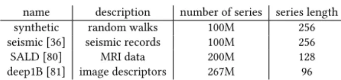
Table 2: Experimental datasets

name description number of series series length

synthetic random walks 100M 256

seismic [36] seismic records 100M 256

SALD [80] MRI data 200M 128

deep1B [81] image descriptors 267M 96

distance, about the relative error of the current progressive result, or about the exact answer itself.

An analyst may choose to stop query execution as soon as the prediction interval of thek-NN distance lies above a low threshold value. Unfortunately, this strategy raises some concerns. Recent work on progressive visualization [59] dis-cusses the problem of confirmation bias, where an analyst may use incomplete results to confirm a “preferred hypothe-sis”. This is a well-studied problem in sequential analysis [82]. It relates to the multiple-comparisons problem [90] and is known to increase the probability of a Type I error (false positives). We evaluate how such multiple sequential tests affect the accuracy of our methods, but discourage their use as stopping criteria, and instead propose the following three.

A sensible approach is to make use of the relative distance error estimate ˆϵQ(t ) (see Eq. 3). For instance, the analyst

may decide to stop the search when the upper bound of the error’s interval is below a thresholdϵ = 1%. An error-based stopping criterion offers several benefits: (i) the choice of a threshold does not depend on the dataset, so its interpretation is easier; (ii) this criterion does not inflate Type I errors as long as the thresholdϵ is fixed in advance; (iii) the error ϵQ(t ) monotonically converges to zero (the same holds for

the bounds of its estimates), thus there is a unique point in timeτQ,θ,ϵat which the bound of the estimated error reaches

ϵ, where 1 − θ is our confidence level (here, θ determines the proportion of times for which the relative distance error of our result will be greater thanϵ).

A second approach is to use theτQ,ϕ bound (see

Sec-tion 4.2) to stop the search, which provides guarantees about the proportion of exact answers, rather than the distance error. It also depends on a single parameter, rather than two. To avoid the multiple-comparisons problem, we provide a single estimate of this bound at the very beginning of the search, allowing users to plan ahead their stopping strategy.

A third approach is to bound the probabilitypQ(t ).

Specifi-cally, we stop the search when this probability exceeds a level

1 −ϕ, where ϕ here represents the probability that the

cur-rent progressive answer is not the exact. We experimentally assess the tradeoffs of these three stopping criteria.

5

PREDICTION METHODS

We now present our solutions. We use the 4 datasets shown in Table 2 to showcase our methods. We further explain and use these datasets in Section 6 to evaluate our methods.

Our goal is to support reliable prediction with small train-ing sets of queries. We are also interested in expresstrain-ing the uncertainty of our predictions with well-controlled bounds, as discussed in the previous section. We thus focus on sta-tistical models that capture a small number of generic rela-tionships in the data. We first examine methods that assume constant information (IQ(t ) = IQ). They are useful for provid-ing an initial estimate before the search starts. We distprovid-inguish between query-sensitive methods, which take into account the query series Q, and query-agnostic methods, which pro-vide a common estimate irrespective ofQ (IQ = I). Inspired

by Ciacca et al. [20, 22], these methods serve as baselines to compare to a new set of progressive methods. Our progres-sive methods update information during the execution of a search, resulting in considerably improved predictions.

To simplify our analysis, we focus on 1-NN similarity

search. Our analysis naturally extends tok-NN search; a

detailed study of this case is part of our future work.

5.1

Initial 1-NN Distance Estimates

We first concentrate on how to approximate the distribution

functionhQ,0(x) (see Equation 4), thus provide estimates

before similarity search starts.

As Ciaccia et al. [20], we rely on witnesses, which are “training” query series that are randomly sampled from a dataset. Unlike their approach, however, we do not use the distribution of raw pairwise distancesFQ(·). Instead, for each

witness, we execute 1-NN similarity queries with a fast state-of-the-art algorithm, such as iSAX2+ [15], or DSTree [85]. This allows us to derive directly the distribution of 1-NN distances and predict the 1-NN distance of new queries.

This approach has two main benefits. First, we use the tree structure of the above algorithms to prune the search space and reduce pre-calculation costs. Rather than calculat-ing a large number of pairwise distances, we focus on the distribution of 1-NN distances with fewer distance calcula-tions. Second, we achieve reliable and high-quality approx-imation with a relatively small number of training queries (≈ 100 − 200) independently of the dataset size (we report and discuss these results in Section 6).

Query-Agnostic Model (Baseline). Let W = {Wj|j =

1..nw}be a set ofnw = |W| witnesses randomly drawn

from the dataset. We execute a 1-NN similarity search for each witness and build their 1-NN distance distribution. We then use this distribution to approximate the overall

(query-independent) distribution of 1-NN distancesдn(·) and its

cumulative probability functionGn(·). This method is

com-parable to Ciaccia et al. [22] query-agnostic approximation method and serves as a baseline.

Query-Sensitive Model. Intuitively, the smaller the dis-tance between the query and a witness, the better the 1-NN

0 2 4 6 8 10 12 0 5 10 15 0 1 2 3 4 5 0 2 4 6 8 10 12 0 1 2 3 4 5 0 2 4 6 8 0 2 4 6 8 0 2 4 6 8 10 12 y = 1.2x + 1.1 R2 = .78 y = 2.3x - 3.3R2 = .37 y = 1.5x - 2.0R2 = .37

seismic SALD deep1B synthetic

Re al 1-NN Dist an ce

Weighted Witness 1-NN Distance

y = 1.4x - 0.5 R2 = .65

Figure 2: Linear models (red lines) predicting the real

1-NN distancedQ,1nn based on the weighted witness

1-NN distancedwQ forexp = 5. All models are based

onnw = 200 random witnesses and nr = 100 queries,

and tested on 500 queries (in orange). The blue dashed lines show the range of their 95% prediction intervals.

of this witness predicts the 1-NN of the query. We capture this relationship through a random variable that expresses

the weighted sum of the 1-NN distance of allnwwitnesses:

dwQ= nw X j=1 (aQ, j·d_W i,1nn) (8)

The weightsaQ, j are derived as follows:

aQ, j = d (Q,Wj) −exp nw P i=1d (Q,Wi) −exp (9)

Our tests have shown optimal results for exponentsexp that

are close to 5. For simplicity, we useexp = 5 for all our

analyses. Additional tests have shown that the fit of the model becomes consistently worse if witnesses are selected with the GNAT algorithm [12, 20] (we omit these results for brevity). Therefore, we only examine random witnesses here.

We usedwQas predictor of the query’s real 1-NN distance

dQ,1nnand base our analysis on the following linear model:

dQ,1nn = β · dwQ + c (10)

Figure 2 shows the parameters of instances of this model for the four datasets of Table 2. We conduct linear regres-sions by assuming that the distribution of residuals is normal (Gaussian) and has equal variance.

Since the model parameters (β and c) and the variance are dataset specific, they have to be trained for each individual dataset. To train the model, we use an additional random sample ofnr training queries that is different from the sample of witnesses. Based on the distance of each training queryQi

from the witnesses, we calculatedwQi (see Equation 8). We

also run similarity search to find its 1-NN distancedQi,1nn.

We then use all pairs(dwQi, dQi,1nn), where i = 1..nr, to

build the model. The approach allows us to construct both point estimates (see Equation 8) and prediction intervals (see Figure 2) that provide probabilistic guarantees about the range of the 1-NN distance.

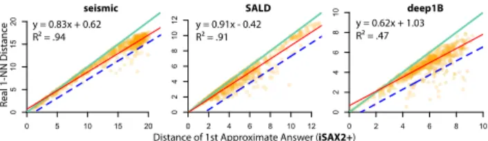
0 5 10 15 20 0 5 10 15 20 0 2 4 6 8 10 12 0 2 4 6 8 10 12 0 2 4 6 8 10 0 2 4 6 8 10 Re al 1-NN Dist an ce

Distance of 1st Approximate Answer (iSAX2+) y = 0.83x + 0.62

R = .94 y = 0.91x - 0.42R = .91

y = 0.62x + 1.03 R = .47

seismic SALD deep1B

Figure 3: Linear models (red solid lines) predicting the

real 1-NN distance dQ,1nn based on iSAX2+ first

ap-proximate answer distance. All models trained with 200 queries. The 500 (orange) points in each plot are queries out of the training set. Green (solid) lines (y = x) are hard upper bounds, set by the approximate an-swer. Blue lines show the range of one-sided 95% pre-diction intervals that form probabilistic lower bounds.

5.2

Progressive 1-NN Distance Estimates

So far, we have focused on initial 1-NN distance estimates. Those do not consider any information about the partial results of a progressive similarity-search algorithm. Now, given Definition 4.1, the distance of a progressive result dQ,R(ti) will never deteriorate and thus can act as an upper

bound for the real 1-NN distance. The challenge is how to provide a probabilistic lower bound that is larger than zero. Our approach relies on the observation that the approxi-mate answers of index-based algorithms are generally close to the exact answers. Figure 3 illustrates the relationship between the true 1-NN distance and the distance of the first progressive (approximate) answer returned by iSAX2+ [15]. (The results for the DSTree index [85] that follows a com-pletely different design from iSAX2+ are very similar; we omit them for brevity). We observe a strong linear relation-ship for both algorithms, especially for the DSTree index. We can express it with a linear model and then derive proba-bilistic bounds in the form of prediction intervals. As shown in Figure 3, the approach is particularly useful for construct-ing lower bounds. Those are clearly greater than zero and provide valuable information about the extent to which a progressive answer can be improved or not.

Since progressive answers improve over time and tend to converge to the 1-NN distance, we could take such informa-tion into account to provide tighter estimates as similarity search progresses. To this end, we examine different progres-sive prediction methods. They are all based on the use of a dataset ofnrtraining queries that includes information about

all progressive answers of a similarity search algorithm to each query, including a timestamp and its distance. Linear Regression. Lett1, t2, ..., tmbe specific moments of

interest (e.g., 100ms, 1s, 3s, and 5s). Giventi, we can build a

time-specific linear model:

wheredQ,R(ti) is Q’s distance from the progressive answer at

timeti. As an advantage, this method produces models that are well adapted to each time of interest. On the downside, it requires the pre-specification of a discrete set of time points, which may not be desirable for certain application scenarios. However, building such models from an existing training dataset is inexpensive, so reconfiguring the moments of in-terest at use time is not a problem.

The above model can be enhanced with an additional termβ · dwQ (see Equation 8) that takes witness information

into account. However, this term results in no measurable improvements in practice, so we do not discuss it further. Kernel Density Estimation. A main strength of the previ-ous method is its simplicity. However, linearity is a strong assumption that may not always hold. Other assumption violations, such as heteroscedasticity, can limit the accuracy of linear regression models. As alternatives, we investigate non-parametric methods that approximate the density distri-bution functionhQ,t(·) based on multivariate kernel density

estimation [27, 83].

As for linear models, we rely on the functional relation-ship between progressive and final answers. We represent this relationship as a 3-dimensional density probability func-tionkQ(x,y, t ) that expresses the probability that the 1-NN

distance fromQ is x, given that Q’s distance from the

pro-gressive answer at timet is y. From this function, we derive hQ,t(x) by setting y = dQ,R(t ).

We examine two approaches for constructing the function kQ(·, ·, ·). As for linear models, we specify discrete moments

of interestti and then use bivariate kernel density estima-tion [84] to construct an individual density probability func-tionkQ(·, ·, ti). Alternatively, we construct a common density

probability function by using 3-variate kernel density esti-mation. The advantage of this method is that it can predict the 1-NN distance at any point in time. Nevertheless, this comes with a cost in terms of precision (see Section 6).

The accuracy of kernel density estimation highly depends on the method that one uses to smooth out the contribution of points (2D or 3D) in a training sample. We use gaussian ker-nels, but for each estimation approach, we select bandwidths with a different technique. We found that the plug-in selector of Wand and Jones [84] works best for our bivariate approach, while the smoothed cross-validation technique [27] works best for our 3-variate approach.

Measuring Time. So far, we have based our analysis on time. Nevertheless, time (expressed in seconds) is not a reli-able measure for training and applying models in practice. The reason is that time largely depends on the available computation power, which can vary greatly across different hardware settings. Our solution is to use alternative mea-sures that capture the progress of computation without being

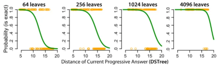
5 10 15 20 .0 .2 .4 .6 .8 1.0 5 10 15 20 .0 .2 .4 .6 .8 1.0 5 10 15 20 .0 .2 .4 .6 .8 1.0 5 10 15 20 .0 .2 .4 .6 .8 1.0 Probability 1-NN found

Probability (is exact)

64 leaves 256 leaves 1024 leaves 4096 leaves

Distance of Current Progressive Answer (DSTree)

Figure 4: Estimating the probability of exact answers with 100 training queries based on the current pro-gressive answer (seismic dataset). We show the logis-tic curves (in green) at different points in time (64, 256, 1024, and 4096 leaves) and 200 test queries (in orange). affected by hardware and computation loads. One can use either the number of series comparisons (i.e., the number of distance calculations), or the number of visited leaves. Both measures can be easily extracted from the iSAX2+ [15], the DSTree [85], or other tree-based similarity-search algo-rithms. Our analyses in this paper are based on the number of visited leaves (Leaves Visited). We should note that for a given number of visited leaves, we only consider a single approximate answer, which is the best-so-far answer after traversing the last leaf.

5.3

Estimates for Exact Answers

We investigate two types of estimates for exact answers (see Section 4.2): (i) progressive estimates of the probability pQ(t ) that the 1-NN has been found; and (ii) query-sensitive

estimates of the timetQ that it takes to find the exact answer.

We base our estimations on the observation that queries with larger 1-NN distances tend to be harder, i.e., it takes longer to find their 1-NN. Now, since approximate distances are good predictors of their exact answers (see previous subsection), we can also use them as predictors ofpQ(t ) and tQ.

Probability Estimation. Lett1, t2, ..., tm be moments of

in-terest, and letdQ,R(ti) be the distance of the progressive

result at timeti. We use logistic regression to model the probabilitypQ(ti) as follows:

ln pQ(ti)

1 −pQ(ti) =βti·dQ,R(ti) + cti (12)

Again, we can use the number of visited leaves to represent time. Figure 4 presents an example for the seismic dataset, where we model the probability of exact answers for four points in time (when 64, 256, 1024, and 4096 leaves are vis-ited). We observe that over time, the curve moves to the right range of distances, and thus, probabilities increase.

Note that we have considered other predictors as well (such as the time passed since the last progressive answer), but they did not offer any predictive value.

Time Bound Estimation. As we explained in Section 4.3,

we provide a single estimate fortQ at the very beginning

0 5 10 15 20 0 5 10 15 0 2 4 6 8 10 12 14 0 5 10 15 0 2 4 6 8 10 0 5 10 15

Leaf Visits (log2)

Distance of 1st Approximate Answer (DSTree)

seismic SALD deep1B

Figure 5: Upper time bounds for exact answers (ϕ = .05). Bounds (in blue) are constructed from 100 queries through quantile regression, where we estimate the 95% quantile of the logarithm of leaf visits as a func-tion of the distance of the 1st approximate answer. the distance of the first approximate answer and the number of leaves (in logarithmic scale) at which the exact answer is found. We observe that the correlation between the two vari-ables is rather weak. However, we can still extract meaningful query-sensitive upper bounds, shown in blue (dashed lines). To construct such bounds, we use quantile regression [49]. This method allows us to directly estimate the 1 −ϕ quantile of the time needed to find the exact answer, i.e., derive the

upper boundτQ,ϕ. As a shortcoming, the accuracy of

quan-tile regression is sensitive in small samples. Nevertheless, we show that 100 training queries are generally enough to ensure high-quality results.

5.4

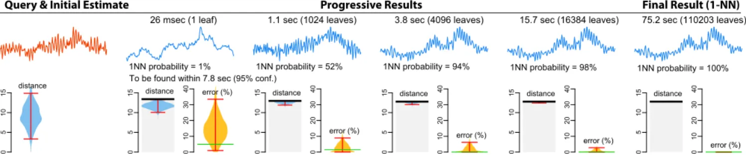
Visualization Example

Figure 6 presents an example that illustrates how the above methods can help users assess how far from the 1-NN their current answers are. We use a variation of pirate plots [70] to visualize the 1-NN distance estimate ˆdQ,1nn(t ) and the

relative error estimate ˆϵQ(t ) by showing their probability

density distribution and their 95% prediction interval. We also communicate the probabilitypQ(ti) and a probabilistic

boundτQ,ϕ(ϕ = .05) after the first visited leaf.

Observe that the initial distance estimate is rather uncer-tain, but estimates become precise at the early stages of the search. The upper bound of the error estimate drops below 10% within 1.1sec, while the probability that the current an-swer is exact is estimated as 98% after 15.7sec (total query execution time for this query is 75.2sec). Such estimates can give confidence to the user that the current answer is very close to the 1-NN. In this example, the 1-NN is found in 3.8sec.

6

EXPERIMENTAL EVALUATION

Environment. All experiments were run on a Dell T630 rack server with two Intel Xeon E5-2643 v4 3.4Ghz CPUs, 512GB of RAM, and 3.6TB (2 x 1.8TB) HDD in RAID0. Implementation. Our estimation methods were implemented in R. We use R’s lm function to carry our linear regression, the ks library [28] for multivariate kernel density estimation, and the quantreg library [32] for quantile regression. We use

a grid of 200 × 200 points to approximate a 2D density distri-bution and a grid of 60 × 180 × 180 points to approximate a 3D density distribution. Source code and datasets are in [1]. Datasets. We used 1 synthetic and 3 real datasets from past studies [30, 92]. All are 100GB in size with cardinalities and lengths reported in Table 2. Synthetic data series were gener-ated as random walks (cumulative sums) of steps that follow a Gaussian distribution (0,1). This type of data has been exten-sively used in the past [15, 33, 93] and models the distribution of stock market prices [33]. The IRIS seismic dataset [36] is a collection of seismic instrument recordings from several stations worldwide (100M series of length 256). The SALD neuroscience dataset [80] contains MRI data (200M series of length 128). The image processing dataset, deep1B [81], con-tains vectors extracted from the last layers of a convolutional neural network (267M series of length 96).

Measures. We use the following measures to assess the estimation quality of each method and compare their results: Coverage Probability: It measures the proportion of the time that the prediction intervals contain the true 1-NN distance. If the confidence level of the intervals is 1 −θ, the coverage

probability should be close to 1 −θ. A low coverage

proba-bility is problematic. In contrast, a coverage probaproba-bility that is higher than its nominal value (i.e., its confidence level) is acceptable but can hurt the intervals’ precision. In particu-lar, a very wide interval that always includes the true 1-NN distance (100% coverage) can be useless.

Prediction Intervals Width: It measures the size of prediction intervals that a method constructs. Tighter intervals are better. However, this is only true if the coverage probability of the tighter intervals is close to or higher than their nominal confidence level. Note that for progressive distance estimates, we construct one-sided intervals. Their width is defined with respect to the upper distance bounddQ,R(t ).

Root-Mean-Squared Error (RMSE): It evaluates the quality of point (rather than interval) estimates by measuring the standard deviation of the true 1-NN distance values from their expected (mean) values.

To evaluate the performance of our stopping criteria, we further report on the following measures:

Exact Answers: It measures the number of exact answers as a percentage of the total number of queries.

Time Savings: Given a load of queries and a stopping criterion, it measures the time saved as a percentage of the total time needed to complete the search without early stopping. Validation Methodology. To evaluate the different meth-ods, we use a Monte Carlo cross-validation approach that consists of the following steps. For each dataset, we randomly draw two disjoint sets of data series Wpooland Tpooland pre-calculate all distances between the series of these two sets. The first set serves as a pool for drawing random sets of wit-nesses (if applicable), while the second set serves as a pool for

26 msec (1 leaf) 1.1 sec (1024 leaves) 3.8 sec (4096 leaves) 15.7 sec (16384 leaves) 75.2 sec (110203 leaves)

0

5

10

15 distance

To be found within 7.8 sec (95% conf.)

0 5 10 15 y distance 1NN probability = 1% 0 10 20 30 40 y error (%) 0 5 10 15 y distance 1NN probability = 52% 0 10 20 30 40 y error (%) 0 5 10 15 y distance 1NN probability = 94% 0 10 20 30 40 y error (%) 0 5 10 15 y distance 1NN probability = 98% 0 10 20 30 40 y error (%) 0 5 10 15 y distance 1NN probability = 100% 0 10 20 30 40 y error (%)

Query & Initial Estimate Progressive Results Final Result (1-NN)

Figure 6: A query example from the seismic dataset showing the evolution of estimates based on our methods. The thick black lines show the distance of the current approximate answer. The red error bars represent 95% prediction intervals. The green line over the predicted distribution of distance errors shows the real error – it is unknown during the search and is shown here for illustration purposes. Estimates are based on a training set of 100 queries, as well as 100 random witnesses for initial estimates. We use the iSAX2+ index.

0

4

8

16

leavesVisited leavesVisited leavesVisited

0

4

8

16

leavesVisited leavesVisited leavesVisited

Le av es V isi ted (log2) 0 4 8 12 16 0 4 8 12 16 (DS Tr ee ) (iSAX2+)

1-NN found search complete

synthetic seismic SALD deep1B

Figure 7: Distribution (over 100 queries) of the number

of leaves visited (inloд2scale) until finding the 1-NN

(light blue) and completing the search (yellow). The thick black lines represent medians.

randomly drawing training (if applicable) and testing queries. At each iteration, we drawnwwitnesses (nw = 50, 100, 200,

or 500) and/ornr training queries (nr = 50, 100, or 200) from

W_pooland Tpool, respectively. We also drawnt = 200 testing

queries from Tpool such that they do not overlap with the

training queries. We train and test the evaluated methods

and then repeat the same procedureN = 100 times, where

each time, we draw a new set of witnesses, training, and testing queries. Thus, for each method and condition, our

results are based on a total ofN × nt = 20K measurements.

For all progressive methods, we test the accuracy of their estimates after the similarity search algorithm has visited 1 (20), 4 (22), 16 (24), 64 (26), 256 (28), and 1024 (210) leaves. Figure 7 shows the distributions of visited leaves for 100 random queries for all four datasets.

6.1

Results on Prediction Quality

Previous Approaches. We first evaluate the query-agnostic and query-sensitive approximation methods of Ciaccia et al. [20, 21]. To assess how the two methods scale with and without sampling, we examine smaller datasets with cardi-nalities of up to 1M data series (up to 100K for the query-agnostic approach). Those datasets are derived from the ini-tial datasets presented in Table 2 through random sampling.

0 20 40 60 80 1K 10K 50K 100K Dataset Cardinality Coverage (%) 1K 10K 50K 100K Dataset Cardinality 0 20 40 60 80 10K 50K 100K 1M

Dataset Cardinality Dataset Cardinality10K 50K 100K 1M

synthetic seismic SALD deep1B Query Agnostic

Full Dataset 10% sample Random Witnesses Query SensitiveGNAT

Figure 8: Coverage probabilities of query-agnostic (left) and query-sensitive (right) methods of Ciaccia et al. [20, 21] for 95% confidence level. We use 500 wit-nesses for the query-sensitive methods. We show

best-case results (with the bestexp: 3, 5, 12, or adaptive).

Such smaller dataset sizes allow us to derive the full distri-bution of distances without sampling errors, while they are sufficient for demonstrating the behavior of the approxima-tion methods as datasets grow.

Figure 8 presents the coverage probabilities of the methods. The behavior of query-agnostic approximation is especially poor. Even when the full dataset is used to derive the distri-bution of distances, the coverage tends to drop below 10% for larger datasets (95% confidence level). This demonstrates that the approximated distribution of 1-NN distances completely fails to capture the real one.

Results for the query-sensitive method are better, but cov-erage is still below acceptable levels. Figure 8 presents results

fornw = 500 witnesses. Note that our further tests have

shown that larger numbers of witnesses result in no or very little improvement, while Ciacca et al. [20] had tested a max-imum of 200 witnesses. To weight distances (see Equation 9),

we tested the exponent valuesexp = 3, 5, and 12, where

the first two were also tested by Ciacca et al. [20], while we found that the third one gave better results for some datasets. We also tested the authors’ adaptive technique. Fig-ure 8 presents the best result for each dataset, most often given by the adaptive technique.

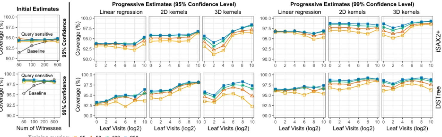
90.0 92.5 95.0 97.5 100.0 50 100 200 500 Num of Witnesses Coverage (%) 90.0 92.5 95.0 97.5 100.0 50 100 200 500 Coverage (%) Initial Estimates 95% Confidence 99% Confidence Query sensitive Query sensitive Baseline Baseline 90.0 92.5 95.0 97.5 100.0 0 2 4 6 8 10 0 2 4 6 8 10 0 2 4 6 8 10 Coverage (%) 90.0 92.5 95.0 97.5 100.0 0 2 4 6 8 10

Leaf Visits (log2) 0Leaf Visits (log2)2 4 6 8 100Leaf Visits (log2)2 4 6 8 10 90.0 92.5 95.0 97.5 100.0 0 2 4 6 8 10

Leaf Visits (log2) 0Leaf Visits (log2)2 4 6 8 100Leaf Visits (log2)2 4 6 8 10

Coverage (%) 90.0 92.5 95.0 97.5 100.0 0 2 4 6 8 10 0 2 4 6 8 10 0 2 4 6 8 10

Linear regression 2D kernels 3D kernels Linear regression 2D kernels 3D kernels

Progressive Estimates (95% Confidence Level) Progressive Estimates (99% Confidence Level)

iSAX2+

DSTree

25 50 100 200

Training queries:

Figure 9: Coverage probabilities of our estimation methods for 95% and 99% confidence levels. We show averages for the four datasets (synthetic, seismic, SALD, deep1B) and for 25, 50, 100, and 200 training queries.

4.0 4.5 5.0 5.5 6.0 50 100 200 500 Num of Witnesses Mean PI Width (95%) 8 10 12 14 50 100 200 500 Num of Witnesses 8 9 10 11 50 100 200 500 Num of Witnesses 4.5 5.0 5.5 6.0 50 100 200 500 Num of Witnesses

synthetic seismic SALD deep1B

25 50 100 200

Training queries:

Figure 10: The mean width of the 95% PI for the witness-based query-sensitive method in relation to the number of witnesses and training queries.

We observe that the GNAT method results in clearly higher coverage probabilities than the fully random method. This result is somehow surprising because Ciacca et al. [20] report that the GNAT method tends to become less accurate than the random method in high-dimensional spaces with more than eight dimensions. Even so, the coverage probability of the GNAT method is largely below its nominal level. In all cases, it tends to become less than 50% as the cardinality of the datasets increases beyond 100K, while in some cases, it drops below 20% (synthetic and seismic).

For much larger datasets (e.g., 100M data series), we expect the accuracy of the above methods to become even worse. We conclude that they are not appropriate for our purposes, thus we do not study them further.

Quality of Distance Estimates. We evaluate the coverage probability of 1-NN distance estimation methods for con-fidence levels 95% (θ = .05) and 99% (θ = .01). Figure 9 presents our results. The coverage of the Baseline method

reaches its nominal confidence level fornw = 200 to 500

witnesses. In contrast, the Query-Sensitive method demon-strates a very good coverage even for small numbers of

wit-nesses (nw = 50) and training queries (nr = 25). However,

as Figure 10 shows, more witnesses increase the precision of prediction intervals, i.e., intervals become tighter while

they still cover the same proportion of true 1-NN distances. Larger numbers of training queries also help.

The coverage probabilities of progressive estimates (Fig-ure 9-Right) are best for the 2D kernel density approach, very close to their nominal levels. Linear regression leads to lower coverage, while the coverage of the 3D kernel density approach is more unstable. We observe that although the accuracy of the models drops in smaller training sets, cov-erage levels can still be considered as acceptable even if the number of training queries is as low asnr = 25.

Figure 11 compares the quality of initial and early (i.e., based on first approximate answer) estimates provided by dif-ferent techniques: (i) Baseline, (ii) Query-Sensitive method, (iii) 2D kernel density estimate for iSAX2+, and (iii) 2D ker-nel density estimate for DSTree. For all comparisons, we set

nw = 500 and nr = 100. For these parameters, the

cover-age probability of all methods is close to 95%. We evaluate the width of their 95% prediction intervals and RMSE. We observe similar trends for both measures, where the query-sensitive method outperforms the baseline. We also observe that estimation based on the first approximate answer (at the first leaf) leads to radical improvements for all datasets. Over-all, the DSTree index gives better estimates than iSAX2+.

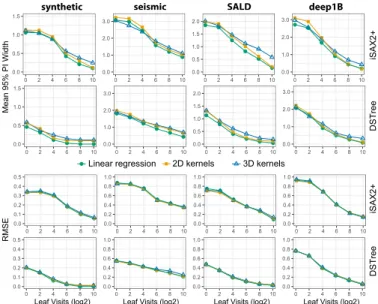
As shown in Figure 12, progressive answers lead to fur-ther improvements. The RMSE is very similar for all three estimation methods, which means that their point estimates are equally good. Linear regression results in the narrowest intervals, which explains the lower coverage probability of this method. Overall, 2D kernel density estimation provides the best balance between coverage and interval width. Sequential Tests. We assess how multiple sequential tests (refer to Section 4) affect the coverage probability of 1-NN distance prediction intervals. We focus on 2D kernel density

estimation (nr = 100), which gives the best coverage (see

0 2 4 6 8 95% PI Width 0 5 10 15 0 2 4 6 8 10 0 2 4 6 8 0.0 0.5 1.0 1.5 2.0 RMSE 0 2 4 6 0 1 2 3 0.0 0.5 1.0 1.5 2.0

Baseline Query Sensitive 1st Leaf - iSAX2+ 1st Leaf - DSTree

seismic SALD deep1B

synthetic

Figure 11: Violin plots showing the distribution of the width of 95% prediction intervals (top) and the distri-bution of the RMSE of expected 1-NN distances

(bot-tom). We usenw = 500 (baseline and query-sensitive

method) andnr = 100 (query-sensitive method and 2D

kernel model for the 1st approximate answer).

seismic SALD iSAX2+ 0.0 0.5 1.0 1.5 0 2 4 6 8 10 0.0 1.0 2.0 3.0 0 2 4 6 8 10 0.0 0.5 1.0 1.5 2.0 0 2 4 6 8 10 0.0 1.0 2.0 3.0 0 2 4 6 8 10 0.0 0.5 1.0 1.5 0 2 4 6 8 10 0.0 1.0 2.0 3.0 0 2 4 6 8 10 0.0 0.5 1.0 1.5 2.0 0 2 4 6 8 10 0.0 1.0 2.0 3.0 0 2 4 6 8 10 Mean 95% PI Width deep1B synthetic 0.0 0.1 0.2 0.3 0.4 0.5 0 2 4 6 8 10 0.0 0.2 0.4 0.6 0.8 1.0 0 2 4 6 8 10 0.0 0.2 0.4 0.6 0.8 1.0 0 2 4 6 8 10 0.0 0.2 0.4 0.6 0.8 1.0 0 2 4 6 8 10 0.0 0.1 0.2 0.3 0.4 0.5 0 2 4 6 8 10

Leaf Visits (log2)

0.0 0.2 0.4 0.6 0.8 1.0 0 2 4 6 8 10

Leaf Visits (log2)

0.0 0.2 0.4 0.6 0.8 1.0 0 2 4 6 8 10

Leaf Visits (log2)

0.0 0.2 0.4 0.6 0.8 1.0 0 2 4 6 8 10

Leaf Visits (log2)

RMSE iSAX2+ DSTree DSTree 3D kernels 2D kernels Linear regression

Figure 12: Progressive models: Mean width of 95% pre-diction intervals of 1-NN distance estimates and RMSE.

Results are based onnr = 100 training queries.

when visiting 1, 512, and 1024 leaves, and (ii) five sequential tests when visiting 1, 256, 512, 768, and 1014 leaves. We count an error if at least one of the three, or five progressive prediction intervals do not include the true 1-NN distance.

As results for DSTree and iSAX2+ were very close, we report on their means (see Figure 13(a)). The coverage of 95% prediction intervals drops from over 95% to about 90% for five tests (higher for seismic and lower for deep1B). Like-wise, the coverage of their 99% prediction intervals drops to around 95%. These results provide rules of thumb on how to correct for multiple sequential tests, e.g., use a 95% level in order to guarantee a 90% coverage in 5 sequential tests. No-tice, however, that such rules may depend on the estimation

deep1B SALD seismic synthetic 95% Level 99% Level 1 3 5 1 3 5 85 90 95 100 Num of Comparisons Coverage (%) 95% Level (φ = .05) 99% Level (φ = .01) 50 100 200 50 100 200 90.0 92.5 95.0 97.5 100.0 Training Queries Exact Answers (%)

(b) Time Bounds Coverage (a) 1-NN Distance Sequential Tests

Figure 13: (a) Effect of 3 and 5 sequential tests on the coverage of 95% and 99% prediction intervals. We use

2D kernels withnr = 100. (b) Coverage of exact

an-swers for time upper bounds (95% and 99% conf. levels).

96 97 98 99 100 .01 .05 iSAX2+ DSTree .01 .05 .01 .05 60 70 80 90 100 Exact Answers (%) iSAX2+ DSTree .01 .05 .01 .05 40 60 80 100 Time Savings (%) ϵ ϵ ϵ < (%) Q deep1B SALD seismic synthetic

Figure 14: Evaluation of the stopping criterion that

bounds the distance error (ϵQ < ϵ). We use 95%

predic-tion intervals (θ = .05) and nr = 100 training queries.

method and the time steps at which comparisons are made. An in-depth study of this topic is part of our future work. Time Bounds for Exact Answers. We are also interested in the quality of time guarantees for exact answers (refer to Section 4.2). We evaluate the coverage of our time bounds for 50, 100, and 200 training queries for confidence levels

95% (ϕ = .05) and 99% (ϕ = .01). Figure 13(b) summarizes

our results. We observe that coverage is good for training samples ofnr ≥100, but drops fornr = 50.

6.2

Results on Time Savings

We compare our stopping criteria (see Section 4.3) and assess the time savings they offer. Figure 14 shows results for our first criterion that bounds the distance error. We consider 16 discrete and uniform momentsti, wheret16is chosen to be

equal to the maximum time it takes to find an exact answer in the training sample. For eachti, we train an individual 2D

kernel density and use 95% prediction intervals (θ = .05) for estimation. The coverage (ratio of queries for whichϵQ < ϵ)

exceeds its nominal level (95%) for all datasets, which sug-gests that results might be conservative. The reason is that stopping could only occur at certain moments. For higher granularity, one can use a larger number of discrete moments.

The ratio of exact answers is close to 95% forϵ = .01 but

becomes unstable forϵ = .05, dropping to as low as 70%

for the seismic dataset. On the other hand, this results in considerable time savings, especially for DSTree: higher than 90% for the synthetic, SALD, and deep1B datasets.