ULF magnetic emissions connected with under sea bottom earthquakes

HAL Id: hal-00301572

https://hal.archives-ouvertes.fr/hal-00301572

Submitted on 1 Jan 2001

HAL is a multi-disciplinary open access

archive for the deposit and dissemination of

sci-entific research documents, whether they are

pub-lished or not. The documents may come from

teaching and research institutions in France or

abroad, or from public or private research centers.

L’archive ouverte pluridisciplinaire HAL, est

destinée au dépôt et à la diffusion de documents

scientifiques de niveau recherche, publiés ou non,

émanant des établissements d’enseignement et de

recherche français ou étrangers, des laboratoires

publics ou privés.

ULF magnetic emissions connected with under sea

bottom earthquakes

V. S. Ismaguilov, Yu. A. Kopytenko, K. Hattori, P. M. Voronov, O. A.

Molchanov, M. Hayakawa

To cite this version:

V. S. Ismaguilov, Yu. A. Kopytenko, K. Hattori, P. M. Voronov, O. A. Molchanov, et al.. ULF

magnetic emissions connected with under sea bottom earthquakes. Natural Hazards and Earth System

Science, Copernicus Publications on behalf of the European Geosciences Union, 2001, 1 (1/2),

pp.23-31. �hal-00301572�

c

European Geophysical Society 2001

Natural Hazards

and Earth

System Sciences

ULF magnetic emissions connected with under sea bottom

earthquakes

V. S. Ismaguilov1, Yu. A. Kopytenko1, K. Hattori2, P. M. Voronov1, O. A. Molchanov4, and M. Hayakawa3 1_{SPbF IZMIRAN, St. Petersburg, Russia}

2_{RIKEN IFREQ, MBRC Chiba University, Chiba, Japan} 3_{UEC, Chofu, Japan}

4_{EORC NASDA, Tokyo, Japan}

Received: 14 May 2001 – Accepted: 25 July 2001

Abstract. Measurements of ULF electromagnetic distur-bances were carried out in Japan before and during a seismic active period (1 February 2000 to 26 July 2000). A network consists of two groups of magnetic stations spaced apart at a distance of ≈ 140 km. Every group consists of three, 3-component high sensitive magnetic stations arranged in a tri-angle and spaced apart at a distance of 4–7 km. The results of the ULF magnetic field variation analysis in a frequency range of F = 0.002−0.5 Hz in connection with nearby earth-quakes are presented. Traditional Z/G ratios (Z is the verti-cal component, G is the total horizontal component), mag-netic gradient vectors and phase velocities of ULF waves propagating along the Earth’s surface were constructed in several frequency bands. It was shown that variations of the R(F ) = Z/Gparameter have a different character in three frequency ranges: F1 = 0.1 ± 0.005, F2 = 0.01 ± 0.005

and F3=0.005 ± 0.003 Hz. Ratio R(F3)/R(F1)sharply

in-creases 1–3 days before strong seismic shocks. Defined in a frequency range of F 2 = 0.01 ± 0.005 Hz during nighttime intervals (00:00–06:00 LT), the amplitudes of Z and G com-ponent variations and the Z/G ratio started to increase ≈1.5 months before the period of the seismic activity. The ULF emissions of higher frequency ranges sharply increased just after the seismic activity start. The magnetic gradient vectors (∇B ≈ 1 − 5 pT/km), determined using horizontal compo-nent data (G ≈ 0.03 − 0.06 nT) of the magnetic stations of every group in the frequency range F = 0.05 ± 0.005 Hz, started to point to the future center of the seismic activity just before the seismoactive period; furthermore they con-tinued following space displacements of the seismic activ-ity center. The phase velocactiv-ity vectors (V ≈ 20 km/s for F = 0.0067 Hz), determined using horizontal component data, were directed from the seismic activity center. Gra-dient vectors of the vertical component pointed to the clos-est seashore (known as the “sea shore” effect). The location of the seismic activity centers by two gradient vectors,

con-Correspondence to: V. S. Ismaguilov

(galina@gh5667.spb.edu)

structed at every group of magnetic stations, gives an ≈10 km error in this experiment.

1 Introduction

On the basis of modern knowledge, one can conclude that the main processes in the Earth’s crust, connected with the earthquake preparation and reflected in ULF electromagnetic fields in a frequency range of f = 0.011 Hz, are the follow-ing: direct ULF radiation from the EQ origin zone (Kopy-tenko et al., 1990, 1993; Fraser-Smith et al., 1990; Bernardy et al., 1991; Molchanov et al., 1992); and the changing of a geoelectric conductivity inside and nearby the EQ hearth zone leads to the changing of amplitudes of reflected elec-tromagnetic waves generated by outer sources (Mogi, 1985; Rokitjanskij, 1975; Kovtun, 1980; Gasanenko, 1963).

Spatial/temporal ULF characteristics observed on the Earth’s surface are fragmental. This is caused by infrequent ULF magnetic measurements in seismic active zones during the earthquakes. Construction of magnetic variation polar-ization (the ratio of the vertical component of the magnetic field variations to the horizontal one), calculated from mag-netic data measured on the Earth’s surface by 3-component magnetometers, is traditional when investigating ULF mag-netic emissions in the seismic active zones. It was shown (Hayakawa et al., 1996a; Hayakawa et al., 1996b; Kopytenko et al., 1999) that there is an increasing of the Z/H ratio be-fore a strong earthquake takes place, and after the earthquake the ratio decreases. We continue to use this method. Time evolutions of the ULF magnetic variation amplitudes before and during seismic active periods were investigated in this work too.

A phase-gradient method (Kopytenko et al., 2000) using three-point measurements of magnetic field variations is ap-plied. A vector of the phase velocity of waves propagating from a source is always directed from the source. A vector of the gradient of the wave intensities is always directed to the source. The method gives an opportunity to construct the

24 V. S. Ismaguilov et al.: ULF magnetic emissions connected with earthquakes 13 0.1 1.0 R= Z /G (rel .u nit s) 2 3 4 5 6 7 EQ mag nit ude 0 50 100 150 EQ nu m (cou nt s) 0 2 4 0 5 10 15 R( F 2) /R (F 1) F1 F2

1-Apr 11-Apr 21-Apr 1-May 11-May 21-May 31-May 10-Jun 20-Jun 30-Jun 10-Jul 20-Jul 30-Jul

0 4 8 12 K-in de x A B C D E Fig.1 Fig.2 Ms=6.4 Izu Chiba 100 km Se Mo Ka ki Uc Un Tokyo

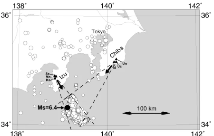
Fig. 1. Location of magnetic stations (black triangles) and seismic

shock epicenters (circles). Black circle is the epicenter of the earth-quake; black arrows represent the direction of the magnetic gradient vectors defined in the frequency range of f = 0.05 ± 0.005 Hz dur-ing the period of 00:00–06:00 LT, 1 July 2000. Dashed lines are gradient cones of the ULF electromagnetic source location. Sym-bols Se, Mo, Ka, U n, U c and Ki represent the first two letters of the names of the magnetic stations.

phase velocity and the gradient vectors along the Earth’s sur-face using three-points measurements. It provides the pos-sibility of finding a direction to the ULF source and of de-terming the position of seismic activity centers, if the ULF disturbances are accompanied by these centers.

2 Experiment

Electromagnetic measurements were performed in a seismi-cally active zone of Japan by two special sets of ground-based gradient installation, spaced about 140 km apart. The special array consists of three MVC-2DS high sensitive tor-sion magnetometers (50 Hz sampling rate, GPS system for data synchronization), arranged in a triangle and spaced ≈ 4– 7 km apart. One set of the magnetometers was installed at the Izu peninsula (Seikoshi, Mochikoshi and Kamo) another one at the Chiba peninsula (Unobe, Kiyosumi and Uchiura). The seismic active period began on 27 June 2000 and lasted more than 2 months. The positions of the magnetic stations and epicenters of the seismic shocks with magnitude M ≥ 2 are shown in the Fig. 1. The size of the circles in Fig. 1 corre-sponds to the magnitude of the seismic shocks. The seismic shocks with the magnitude M ≥ 2 were taken into consider-ation in this work since the shocks with smaller magnitudes were not observed at the recordings of the closest magnetic station (Kamo). The strongest shock (EQ) had the magnitude M = 6.4. The epicenter of this EQ was situated at a depth of ≈ 15 km under the sea surface at a distance of ≈ 80 km to the southeast from the magnetic stations located at the Izu peninsula and ≈ 140 km to the southwest from the magnetic stations located at the Chiba peninsula.

3 Data processing and results

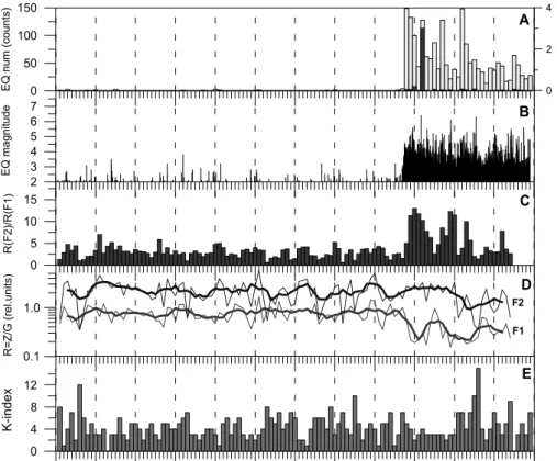
Magnetic data from the Mochikoshi station were used for the construction of Fig. 2. This figure presents a connection of the magnetic field component ratios with the seismic activ-ity. The number of seismic shocks during 6-hour intervals of every day (00:00–06:00 LT) during the period from 1 April to 27 July 2000 are shown as columns with a light color in the top panel (a) of Fig. 2. Columns with a dark color in the same panel correspond to the energy of the shocks with M > 2 summarized in every time interval. The energy of EQ was calculated according with the formula

log(E) = α + βM (1)

where E is EQ energy, and M is a magnitude of the EQ. Coefficients α = 12.32 and β = 1.42 were proposed in Mogi (1985) and King et al. (1969). Most of the EQ energy was selected on 1 July 2000 and is connected to the strongest EQ.

The seismic shocks with M ≥ 2 are plotted in panel (b). Only shocks with epicenters situated closer than 120 km from the Mochikoshi station were taken into account. Strong seis-mic activity began on 27 June 2000 at ≈ 15:00 LT and lasted more than 3 months. The strongest EQ (M = 6.4) took place on 1 July 2000 at 16:01:56 LT.

The lowest panel (e) in Fig. 2 presents K indexes cal-culated at the Kakioka observatory and summarized during the same time intervals (00:00–06:00 LT). The nighttime in-tervals were chosen due to the lower level of the industrial noise. Strong magnetic storms occured on 6 April, 5 May, 23 May, 9 June, 12 June, 15 June and 15 July.

The magnetic component ratios R = Z/G are marked in panel (d) of Fig. 2 as F1and F2. Symbol Z means the

ver-tical component and G represents the total horizontal com-ponent. The lower curve in panel (d) presents the Z/G ratio in the frequency range of F1=0.0950.105 Hz and the upper

curve is the same ratio but for the lower frequency range of F2 =0.0020.008 Hz. These ratios and power spectra

densi-ties in frequency range F = 0.002 − 0.2 Hz were obtained using the maximum entropy spectral method. It is clearly seen that F1 curve values sharply decrease just before the

beginning of the seismic activity. F2 curve values have no

strong variation associated with the seismic activity, but the variations have a good correlation with the magnetic activity plotted in the lowest panel. The parameter R(F2)decreases

when the magnetic activity increases.

The histogram in panel (c) is a ratio of the values of R(F2)

and R(F1) plotted in panel (d). This parameter was

con-structed to emphasize the difference in time behaviour of these curves. As seen from this panel, the length of the histogram columns decrease when the magnetic activity in-creases.

Time evolutions of the emissions of the total horizontal magnetic field component G and Z/G ratios before and dur-ing the seismic active period (1 February to 26 July 2000) in 4 narrow-band ranges (from 0.002 to 0.2 Hz) are plotted

V. S. Ismaguilov et al.: ULF magnetic emissions connected with earthquakes 25 13 0.1 1.0 R= Z /G (rel .u nit s) 2 3 4 5 6 7 EQ mag nit ude 0 50 100 150 EQ nu m (cou nt s) 0 2 4 0 5 10 15 R( F 2) /R (F 1) F1 F2

1-Apr 11-Apr 21-Apr 1-May 11-May 21-May 31-May 10-Jun 20-Jun 30-Jun 10-Jul 20-Jul 30-Jul 0 4 8 12 K-in de x A B C D E Fig.1 Fig.2 Ms=6.4 Izu Chiba 100 km Se Mo Ka ki Uc Un Tokyo

Fig. 2. Comparison of magnetic field component ratios Z/G with seismic activity in two frequency ranges of F1 = 0.1 ± 0.005 and

F2=0.005 ± 0.003 Hz (Mochikoshi st., Japan, 2000). (A) The number of EQ during 6-hour intervals (00:00–06:00 LT) for every day (light

color) and summary of the energy of earthquakes in these time intervals (dark color); (B) The magnitudes of the earthquakes with M > 2;

(C) The ratio of the two curves from panel (D) with R(F2)/R(F1); (D) The magnetic field component ratios (R = Z/G) in two frequency

ranges of F1and F2, where bold curves are 5-day running means; (E) The K-indexes of the Kakioka magnetic station (sums in intervals

00:00–06:00 LT).

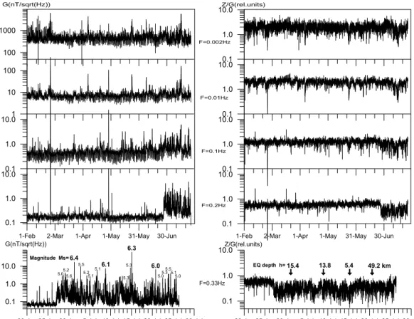
in the upper part of Fig. 3. The time evolutions for the fre-quency f = 0.33 ± 0.03 Hz are presented in the lower part of the figure for a shorter time interval (20 June to 27 July 2000). The numbers in the lower part represent the seismic shock magnitudes (left side) and the seismic shock depths (right side). EQ with M = 6.3 produces a maximal mag-netic effect in the higher frequency range, probably due to the smallest depth (5.4 km). The effect of a strong magnetic storm is clearly seen in the lower frequency ranges just af-ter this EQ. The curves in Fig. 3 were constructed using the spectral maximum entropy method. The increasing of the G component amplitude and the Z/G ratio decreasing are seen just before the start of the seismic activity in the higher fre-quency ranges of 0.1, 0.2 and 0.33 Hz. The lower frequen-cies have none of the same sharp features connected with the seismic activity beginning, but the amplitude of the G component and the Z/G ratio both have noticeable 20-day variations before the seismic activity start. Two to three days before the strongest seismic shocks (M > 6.0), we observe a considerable increase in the emission intensities in the higher frequencies. These amplitude intensifications can possibly be the short-term precursors of strong earthquakes.

Time evolutions of the magnetic field amplitudes, gradi-ents and Z/G ratios are presented in Fig. 4. The data of the magnetic field variations from three stations (Seikoshi, Mochikoshi and Kamo) were used. The data were prelimi-nary filtered by a pass-band digital filter in a frequency range of F = 0.005 ± 0.003 Hz. Each panel in the figure contains 3 curves marked by the symbols S, M, K, which represent the first letter of the magnetic station name. The three upper panels of Fig. 4 present the time evolution of the RMS values of the vertical (Z), and the total horizontal (G) components of the magnetic field variations and the Z/G ratio. The RMS values were calculated for 6-hour nighttime intervals (00:00– 06:00 LT,) using the whole period under investigation.

As seen from Fig. 4, the amplitudes of the magnetic field variations have a tendency to increase with time. The in-creasing had started ≈ 1.5–2.0 months before the seismic ac-tive period and changed from ≈ 0.15 up to ≈ 0.2 nT in the Z component and from ≈ 0.07 to ≈ 0.08 nT in the G com-ponent. The increasing in the vertical component is more pronounced than in the total horizontal component. This fact is reflected in the Z/G ratio (upper most panel). One can see an increase in this ratio before the seismic active period.

26 V. S. Ismaguilov et al.: ULF magnetic emissions connected with earthquakes

14

1-Feb 2-Mar 1-Apr 1-May 31-May 30-Jun

0.1 1.0 10.00.1 1.0 10.01 10 100 100 1000 F=0.2Hz F=0.1Hz F=0.01Hz F=0.002Hz

1-Feb 2-Mar 1-Apr 1-May 31-May 30-Jun

0.1 1.0 10.00.1 1.0 10.00.1 1.0 10.00.1 1.0 10.0 G(nT/sqrt(Hz)) Z/G(rel.units)

20-Jun 25-Jun 30-Jun 5-Jul 10-Jul 15-Jul 20-Jul 25-Jul 30-Jul 0.1

1.0 10.0

20-Jun 25-Jun 30-Jun 5-Jul 10-Jul 15-Jul 20-Jul 25-Jul 30-Jul 0.1 1.0 10.0 F=0.33Hz 6.4 6.3 6.1 6.0 5.05.2_5.6 5.5 5.2 5.1 5.1 5.3 5.3 5.05.3 5.5 5.1 5.0 G(nT/sqrt(Hz)) Z/G(rel.units) 15.4 13.8 5.4 49.2 km Magnitude Ms= EQ depth h=

1-Apr 21-Apr 11-May 31-May 20-Jun 10-Jul 30-Jul

-100 -50 0 50 100 dZ (p T /( km (H z) ) -50 0 50 dG (p T /( km (H z) ) N S E W K-M K-S M-S K-M K-S M-S 0.1 0.2 0.3 Z( nT ) 0.0 0.1 0.2 G( nT ) 2 3 4 Z/ G MK S K M S K S M Seismic active period

Fig.3

Fig.4

Fig. 3. Time evolutions of the total horizontal magnetic field component G and the Z/G ratios before and during the seismic active period of

1 February to 26 July 2000 in 4 narrow-band frequency ranges (upper part). Time evolution of the total horizontal magnetic field component

Gand the Z/G ratios for frequency F = 0.33 ± 0.03 Hz during the period of 20 June to 27 July 2000 (lower part). Japan, st. Mochikoshi.

The two lowest panels in Fig. 4 present the time be-haviour of the gradients of the G component of the mag-netic field variations in the directions of Kamo-Seikoshi, Mochikoshi-Seikoshi, Kamo-Mochikoshi for the same night-time intervals. The gradients were calculated using the spec-tral method. The square roots of the Z and G compo-nents power spectral density, calculated for the same 6-hour nighttime intervals, were integrated in the frequency band of F =0.01 ± 0.005 Hz after those differences were calculated for the pairs of magnetic stations: Mochikoshi, Kamo-Seikoshi, Mochikoshi-Seikoshi. The vectors of the gradients were approximately pointed to the north at the beginning of May 2000 (two months before the seismic activity start) and to the southeast at the beginning of June 2000 (three weeks before the seismic activity start). The southeast direction is the direction of the future seismic activity region. To delete the occasional jumps in the results plotted in Fig. 4, three-point median filtering was used. All curves in Fig. 4 are 20-day running means.

4 Phase-gradient method of data processing

Three, 3-component magnetic stations arranged in a trian-gle and spaced about 4–7 km apart provide an opportunity to construct vectors of phase velocities of the ULF magnetic

waves propagating from a source and the magnetic field gra-dients along the Earth’s surface. Any two pairs of magnetic stations can be used for the vector calculations.

Suppose we choose the following coordinate system: X axis is directed from magnetic station 1 to station 2, Y axis is orthogonal to the X axis and directed along the Earth’s surface toward station 3, Z axis is a vertical one and directed downward. Let us choose the following two pairs of stations: 1–2 and 1–3. In this case, for the phase velocity vector, we have: α = ±arccos " V31cos(β) q V2₂₁+V2₃₁−2V21V31sin(β) # |V | = V21cos(α) = V31sin(α + β) (2)

For the gradient vector:

α = ±arccos " G21cos(β) q G2 21+G231−2G21G31sin(β) # |G| = G21cos(α) = G31sin(α + β) (3)

The angle α in Eqs. (2) and (3) is the angle between the X axis and the directions of the vectors. The angle β is the angle between the Y axis and a line connecting stations 1 and 3. In Eqs. (2) and (3), V21, V31 values (phase velocities in

V. S. Ismaguilov et al.: ULF magnetic emissions connected with earthquakes 27 the direction from station 2 to the station 1 and from station 3

to station 1) and G21, G31values (gradients in the directions

from station 2 to station 1 and from the station 3 to station 1 can be defined in the following way:

V21 =d21/T21, V31=d31/T31,

G21=1 B21/d21, G31 =1B31/d31 (4)

where d21, d31represent the distances between the magnetic

stations situated at points 2 and 1, 3 and 1, respectively; T21,

T31are the time (phase) shifts of the ULF geomagnetic

pulsa-tions between the magnetic stapulsa-tions 2 and 1, 3 and 1, respec-tively; 1B21, 1B31 represent the values of the differences

(taking into account the phase shifts) between stations 2 and 1, 3 and 1 in any magnetic field component, respectively. For the geomagnetic coordinate system, similar formulas were reported in Kopytenko et al. (2000).

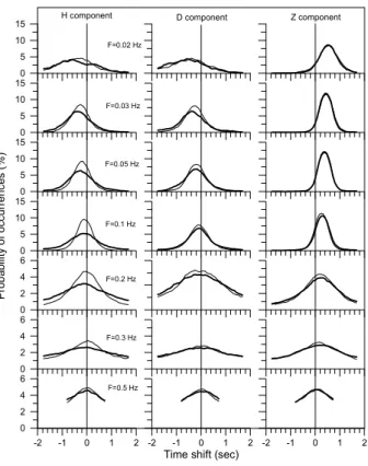
The phase shift distributions are plotted in Fig. 5. Ini-tial data were preliminary filtered by pass-band filters with central frequencies shown in the figure and a half-width of 0.005 Hz. The phase shifts of magnetic field variations be-tween pairs of magnetic stations were defined for the night-time intervals 00:00–06:00 LT. The length of the data win-dow for the determination of the time shifts and gradients was T = 5/fc(fc is the central frequency of the pass-band

filter). The data window moved along the 6-hour data real-ization with a step equal to half of the window.

Maximums of the time shift distributions (most probable values) have a negative sign for the horizontal component of the magnetic field variations and a positive sign for the ver-tical component, as can be seen from Fig. 5. This means that the horizontal component waves of the ULF magnetic field variations propagate primarily in the direction from Mochikoshi to Seikoshi (from southeast to northwest), but the waves in the Z component propagate in the opposite di-rection. Thin curves present the phase distributions in the time interval 00:00-06:00 LT 26 June 2000 (just before the beginning of the seismic active period), and bold curves were plotted for the time interval 00:00–06:00 LT, 1 July 2000 (during the seismic active period). The influence of the seis-mic activity itself is seen in the broadening of the distribu-tions. It can be connected to the increase in the seismic active region size and to the probable increase in the ULF source size. There are no seismic shacking effects in the investigated frequency range, since we do not observe an additional max-imum at the ≈ −0.5 s shift. The shift has to arise at the phase distributions as a time interval of the seismic wave propaga-tion between the two magnetic stapropaga-tions.

The horizontal component curves in Fig. 5 have the dis-tributions with a larger half-width during the seismic active period. The influence of the seismic activity in the verti-cal component phase shift distributions is very small. The time shifts depend on the frequencies: the longer the period is of the magnetic field variations, the higher the absolute value of the time shift. The dependence between the time shifts and the frequencies is approximately the following -1 t ≈ F−1/2. Hence, the phase velocity values of the elec-tromagnetic waves along the Earth’s surface have the inverse

14

1-Feb 2-Mar 1-Apr 1-May 31-May 30-Jun

0.1 1.0 10.00.1 1.0 10.01 10 100 100 1000 F=0.2Hz F=0.1Hz F=0.01Hz F=0.002Hz

1-Feb 2-Mar 1-Apr 1-May 31-May 30-Jun

0.1 1.0 10.00.1 1.0 10.00.1 1.0 10.00.1 1.0

20-Jun 25-Jun 30-Jun 5-Jul 10-Jul 15-Jul 20-Jul 25-Jul 30-Jul

0.1 1.0 10.0

20-Jun 25-Jun 30-Jun 5-Jul 10-Jul 15-Jul 20-Jul 25-Jul 30-Jul

0.1 1.0 10.0 F=0.33Hz 6.4 6.3 6.1 6.0 5.05.2_5.6 5.5 5.2_5.15.1 5.3 5.3 5.05.3 5.5 5.1 5.0 G(nT/sqrt(Hz)) Z/G(rel.units) 15.4 13.8 5.4 49.2 km Magnitude Ms= EQ depth h=

1-Apr 21-Apr 11-May 31-May 20-Jun 10-Jul 30-Jul

-100 -50 0 50 100 dZ (p T /( km (H z) ) -50 0 50 dG (p T /( km (H z) ) N S E W K-M K-S M-S K-M K-S M-S 0.1 0.2 0.3 Z( nT ) 0.0 0.1 0.2 G( nT ) 2 3 4 Z/ G M K S K MS K S M Seismic active period

Fig.3

Fig.4

and the Z/G ratios before and during the seismic active period at 3 magnetic stations (Mochikoshi, Seikoshi and Kamo, 1 April to 27 July 2000). The frequency range is F = 0.005 ± 0.003 Hz. Symbols K, M, S represent the results of the data processing using Kamo, Mochikoshi, Seikoshi data. Vertical dashed line represents the moment when the seismic activity starts. Arrows at the second from the bottom panel show the directions of the total horizontal component gradients. All curves are 20-day running means.

dependence. It corresponds to the well-known expression (Kovtun, 1980) for the phase velocity of the electromagnetic plane waves: V = 103(10ρF )1/2(F is a frequency and ρ is an apparent resistivity).

An example of the amplitude and magnetic gradient sta-tistical distributions is presented in Fig. 6. Maximums of the distributions are the most probable values of the ampli-tudes and gradients. The histograms were constructed for the time interval of 00:00–06:00 LT, 26 June 2000. The raw data were preliminary filtered by the pass-band filter (F = 0.05 ± 0.005 Hz). The amplitude (peak-to-peak val-ues) distributions of the total horizontal component (G = H sin α + D cos α, α = arctan(H /D)) at the Izu and Chiba peninsulas are plotted in the left part of the figure. The most probable amplitude values are ≈ 0.035 nT (Chiba) and ≈0.065 nT (Izu). The gradient distributions are plotted in the right side of Fig. 6. The negative sign of the gradient values means that the gradient vector is directed from Seikoshi to Mochikoshi (Izu), and from Unobe to Kiyosumi (Chiba). As seen from Fig. 6, the gradient vectors of the total horizontal component are directed to the southeast from Izu and to the

28 V. S. Ismaguilov et al.: ULF magnetic emissions connected with earthquakes 15 -2 -1 0 1 2 0 2 4 6 -2 -1 0 1 2

Time shift (sec) -2 -1 0 1 2 0 2 4 6 0 2 4 6 0 5 10 15 P ro b ab ilit y of oc cu rr enc es (%) 0 5 10 150 5 10 150 5 10

15 H component D component Z component

F=0.02 Hz F=0.03 Hz F=0.05 Hz F=0.1 Hz F=0.2 Hz F=0.3 Hz F=0.5 Hz

Fig.5

tion from st. Seikoshi to st. Mochikoshi for 3 magnetic field com-ponents in 7 frequency ranges. Thin curves are plotted for period of 00:00–06:00 LT, 26 June 2000 (before the start of the seismic active period), bold curves represent the period of 00:00–06:00 LT, 1 July 2000 (during the seismic active period). All curves are 7-point run-ning means.

southwest from Chiba (to the side of the seismic activity zone in both cases), but the gradient vectors of the vertical com-ponent are directed to the northwest from Izu group of the stations (to the closest seashore). Z gradients at Chiba had values close to zero in the direction from Unobe to Kiyosumi. A line connecting Unobe and Kiyosumi stations is approxi-mately parallel to the closest seashore; hence, the “seashore” effect does not produce outstanding gradients in this direc-tion.

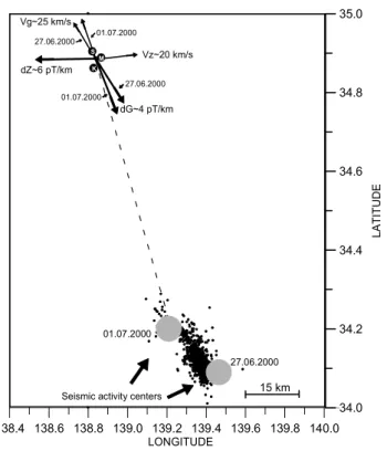
Figures 5 and 6 were constructed using one pair of the magnetic stations from two groups at Izu and Chiba: Seikoshi-Mochikoshi or Unobe-Kiyosumi. Using three-point measurements at any group of magnetic stations, we can calculate the total horizontal (along the Earth’s surface) vectors of the phase velocities and gradients of the magnetic variations in accordance with the Eqs. (2–4). These vectors for the ULF emissions with a period of T = 15 s for the time interval 00:00–06:00 LT, 27 June and 1 July 2000 are plotted in Fig. 7 using the data from the Izu group of stations. Seis-mic activity centers were defined using epicenters of the seis-mic shocks with M > 3. Black points mark the epicenters. Grey circles mark the activity centers. These centers shifted at a distance of ≈ 15 km during 5 days, as can be seen from

16 0 40 80 120 160 200 Amplitude of G comp. (pT) 0 2 4 6 8 Probability of occurrences (%) 0 2 4 6 8 -20 -10 0 10 20 Gradient (pT/km) 0 5 10 15 20 25 Probability of occurrences (%) 0 5 10 15 20 25 Izu Chibo

Seikoshi - Mochikoshi (Izu)

G comp. Z comp.

Unobe - Kiyosumi (Chibo)

G comp. Z comp. 138.4 138.6 138.8 139.0 139.2 139.4 139.6 139.8 140.0 140.2 LONGITUDE K 27.06.2000 01.07.2000

Seismic activity centers 15 km

M Vz~20 km/s S S Vg~25 km/s dG~4 pT/km dZ~6 pT/km 27.06.2000 01.07.2000 27.06.2000 01.07.2000 34.0 34.2 34.4 34.6 34.8 35.0 LA TI T U D E Fig.6 Fig.7

Fig. 6. Distributions of the total horizontal component amplitudes

(left) and the magnetic field gradients (right) at the Izu and Chiba peninsulas for the geomagnetic variations (F = 0.05 ± 0.005 Hz) during the period of 00:00–06:00 LT, 26 June 2000. The black color represents the total horizontal component, thegrey color represents the vertical component.

Fig. 7. On the 27 June 2000, the gradients and phase veloc-ity vectors at Izu rotated 01.07 relatively counterclockwise at an ≈ 100 angle accordingly to the seismic activity cen-ters displacement. We can see that the horizontal component gradient vectors are directed to the source of the ULF emis-sions. The phase velocity vectors of the ULF waves point in the direction from the source. The vertical component vec-tors point to the closest seashore situated at ≈ 5 km from the Seikoshi magnetic station despite a good correlation between the ULF variations in the Z and G magnetic components.

5 Discussion

The results of the investigation of the ULF magnetic distur-bances are presented in Figs. 2 to 4. It is clearly seen that the disturbances with periods close to T = 100 s have the usual “precursor” behaviour where the Z/G ratio started to increase ≈ 1 month before the seismic activity and the ra-tio then decreased during the seismic activity (Hayakawa et al., 1996a, 1996b; Kopytenko et al., 1999). The emission amplitudes in the total horizontal and vertical components have a clear increase during ≈ 1.5 months before the seismic shocks begin (Fig. 4). The disturbances of the longer period (T = 200 s) have not the same peculiarity during this event.

The ULF emissions with a shorter period (T = 10 s) have a different time evolution that was not observed earlier. We can see from Fig. 2 (curve F1) that just before the seismic

active period, the Z/G ratio of these emissions (parameter R(F1)) decreases, while the parameter R(F2)has very small

variations. The ratio R(F2)/R(F1)has sharp variations after

the beginning of the seismic active period (the middle panel in Fig. 2). Strongest seismic shocks are followed by the max-imal values of this ratio except EQ with M = 6.0 (probably due to big EQ depth of 49.2 km). Therefore, the variations

V. S. Ismaguilov et al.: ULF magnetic emissions connected with earthquakes 29 in the R(F ) = Z/G parameter have a different character in

three frequency ranges: F1=0.02 − 0.5, F2=0.01 ± 0.005

and F3=0.005 ± 0.003 Hz. The ratio R(F3)/R(F1)sharply

increases after the beginning of strong seismic activity. This phenomenon is probably caused by the intensive ULF elec-tromagnetic radiation from the seismic source. As seen in Fig. 2, the strong magnetic storm influence leads to a de-creasing of the Z/G ratios in the longest period range.

The essence of this effect has become clear after an inves-tigation of the results presented in Figs. 5 to 7. As it was reported in the previous sections, the phase-gradient method provides the opportunity to find the vectors of the phase ve-locities of ULF waves propagating along the Earth’s surface and their magnetic gradients by using the special magne-tometer array (three, 3-component magnetic stations situated at the top of the triangle and spaced a small distance apart). To find the most probable values, the statistical distributions of the phase and magnetic gradients were constructed simi-larly to the distributions presented in Figs. 5 and 6. Using the horizontal component vectors, we can find the direction of the ULF source from the Izu and Chiba peninsulas. This pro-cedure can be called “magnetic location” of the ULF electro-magnetic sources. The black arrows in Fig. 1 show electro-magnetic gradient directions from Izu and Chiba. The dashed lines in Fig. 1 present the gradient cones used for the magnetic location in the frequency range of F = 0.067 ± 0.005 Hz. The most probable values of the gradients were found from the statistical gradient value distribution constructed for pe-riod of 00:00–06:00 LT, 1 July 2000. The cone borders were determined using half of the distribution heights. It is clearly seen that the location area covers the region of the seismic shock epicenters. The location area center is a 5– 10 km distance from the strongest earthquake with magni-tude M = 6.4. Therefore, we can propose that the seismic hearth is the source of the ULF electromagnetic disturbances in a wide frequency range.

The magnetic gradient of the ULF disturbances in the ver-tical component is directed to the closest seashore (Fig. 7); we probably observe a so-called “seashore” effect. The phase velocity vector in the Z component is directed from the shore. The directions of the phase velocity and gradient vec-tors do not coincide with the Z and G components, but the magnetic variations (the wave forms) in all the components are well correlated. This means that they have a common primary source. We suppose that the vertical magnetic com-ponent variations were caused by induction currents in sea water (sea depth is more than 1 km to the west of the Izu peninsula). The currents are inducted by the horizontal com-ponent variations (orthogonal to the seashore) propagating from the seismic source region and they produce magnetic field variations just in the Z component.

As seen from Fig. 6, the most probable amplitudes (peak-to-peak values) of the ULF signal are ≈ 0.035 nT at Chiba (distance from the center of the seismic activity ≈ 135 km) and ≈ 0.060 nT at Izu (distance from the seismic activity cen-ter ≈ 85 km). If we neglect a damping in the Earth’s crust, we can assume that the amplitude of the ULF emissions changes

16

0

40

80

120

160

200

Amplitude of G comp. (pT)

0

2

4

6

8

Probability of occurrences (%)

0

2

4

6

8

-20

-10

0

10

20

Gradient (pT/km)

0

5

10

15

20

25

Probability of occurrences (%)

0

5

10

15

20

25

Seikoshi - Mochikoshi (Izu)

G comp. Z comp.

Unobe - Kiyosumi (Chibo)

G comp. Z comp. 138.4 138.6 138.8 139.0 139.2 139.4 139.6 139.8 140.0 140.2 LONGITUDE K 27.06.2000 01.07.2000

Seismic activity centers 15 km

M Vz~20 km/s S S Vg~25 km/s dG~4 pT/km dZ~6 pT/km 27.06.2000 01.07.2000 27.06.2000 01.07.2000 34.0 34.2 34.4 34.6 34.8 35.0 LA TI T U D E

Fig.6

Fig.7

Fig. 7. Vectors of gradients and phase velocities of ULF magnetic

emissions (F = 0.067 Hz). Black circles (with the letters S, M,

Kinside) represent the magnetic stations Seikoshi, Mochikoshi and

Kamo. Black points represent the epicenters of seismic shocks with magnitudes M > 3 for the time period 27 June to 2 July 2000. The letters V g (for the total horizontal component) and V z (for the vertical component) mark the vectors of the phase velocities along the Earth’s surface. The vectors of the gradients are marked by the letters dG and dZ. The grey circles represent the seismic activity centers on 27 June and 2 July 2000. The dashed line connects the magnetic stations and the epicenter of the strongest EQ with M = 6.4.

with the distance from the source as ≈ 1/R. A simple de-pendence can be proposed:

B(R) = A0exp(−f βR)/R (5)

where B is the ULF emission amplitude; R is the distance from the source center; A0and β are the parameters

depend-ing on the intensity of the source and dampdepend-ing in the Earth’s crust; f is the frequency of the electromagnetic wave. By using Eq. (5) and the amplitude values from Fig. 6, we can find that for the frequency of F = 0.05 Hz, the amplitude value equals ≈ 1.2 nT at the 5 km distance from the center of the ULF source (approximately at the border of the seismic activity region) and ≈ 0.6 nT at the distance 10 km. Simi-lar values were observed near the Loma-Prietta EQ epicenter (Fraser-Smith et al., 1990; Bernardy et al., 1991).

A ULF generation mechanism can be connected with a re-gion where the intense producion of microcracks in the seis-mic activity hearth takes place(Molchanov and Hayakawa, 1994a, 1994b, 1998). Observed from a large distance, the magnetic field component of the ULF emissions has to de-pend on the orientation of the microcracks (Molchanov and

30 V. S. Ismaguilov et al.: ULF magnetic emissions connected with earthquakes Hayakava, 1998). In the investigated event, we primarily

ob-served the horizontal component. This means that the micro-cracks have primarily opened in the vertical direction. Any local closed configuration of currents inside a seismic active region cannot produce the magnetic field emissions depend-ing on the distance as 1/R. The production of such a depen-dence can be received if the electric charge acceleration is the mechanism of the electromagnetic emissions. Movement of the walls accelerates the electric charges in the microcrack walls during the microcrack’s opening process and transverse electromagnetic fields are then radiated. These fields will change with a distance as 1/R. The model of the electric dipole oscillations was reported by Warwick et al. (1982) and Gershenzon et al. (1989).

Unfortunately, the frequencies (f > 1 MHz) in this gen-eration mechanism are top high, as discussed by Molchanov and Hayakawa (1998). The frequencies of the electromag-netic waves can be much lower if we assume that the electro-magnetic fields are produced by the acceleration of charged water dust and small particles that arise from inside the mi-crocracks during the opening process. The charged parti-cles will be accelerated during the time when the electric charge exists inside the microcrack walls, or during the time when the conductive currents exist, which destroy the micro-crack walls charge. As reported in Molchanov and Hayakawa (1998), this time is > 10−3s (the time depends on a size of the microcracks and a conductivity of a media around the microcracks); hence, it leads to lower frequencies than those in the models of Warwick et al. (1982); and Gershenzon et al. (1989). In the proposed generation mechanism, the ver-tical direction of the microcrack’s opening is also necessary to receive at a large distance the horizontal magnetic field component of the emissions.

A mechanism of the ULF electromagnetic field genera-tion, associated with the deformation of a solid, was pro-posed in Vallianatos and Tzanis (1998, 1999a, 1999b) and Tzanis et al. (2000). The solid deformation generates electric currents. Therefore, we can observe ULF electromagnetic waves outside the deformation zone. But in this case, the ULF emission amplitudes will change with a distance from the source close to the 1/R law, only if the size of the current system will be much more than a distance from the current system to the observational points.

6 Summary

The next properties of the ULF emissions can be defined: – The emissions arise just before and during the seismic

activity period;

– The waveform of the emissions looks like a wide-band electromagnetic noise;

– The horizontal magnetic component of the emissions was primarily observed at the Izu and Chiba peninsu-las during the investigated event;

– The ULF variations in the vertical magnetic component were caused by induction currents in sea water (the sea depth is more than 1 km near the Izu peninsula); – The emission amplitudes increase with frequency

in-creasing;

– The emission amplitudes have a distance dependence of

≈1/R.

Long-period variations in the amplitudes of the ULF dis-turbances in the Z and G magnetic field components and the increasing of the Z/G ratio before the seismic active period can serve as middle-term predictors of a strong EQ. The am-plitude intensifications of the ULF emissions in frequencies of 0.5–0.05 Hz can be the short-term precursors of strong earthquakes.

As it was shown in this work, the direction of the gradient and the phase velocity vectors of the ULF magnetic distur-bances, calculated in the way described above, points to the region of the EQ preparation. Two groups of magnetic sta-tions spaced at a distance of 50-150 km provide the opportu-nity to locate this region at distances of ≤ 100 km from the magnetic stations. Using the observations of the ULF elec-tromagnetic disturbances and the suggested method of the magnetic location of the ULF electromagnetic sources are very important for EQ predictions since many strong EQs have no foreshocks (Mogi, 1985).

References

Bernardy, A., Fraser-Smith, A. C., McGill, P. R., and Villard, Jr., O. G.: ULF magnetic field measurements near the epicenter of the

Ms = 7.1 Loma Prieta earthquake, Phys. Earth. Planet. Inter.,

68, 45–64, 1991.

Fraser-Smith, A. C., Bernardy, A., McGill, P. R., Ladd, M. E., Helli-well, R. A., and Villard, Jr., O. G.: Low frequency magnetic field measurements near the epicenter of the Loma-Prieta earthquake, Geophys. Res. Lett., 17, 1465–1468, 1990.

Gasanenko, L. B.: Impedance of ULF direct line current field sit-uated above earth. In: ‘Electromagnetic sounding and magne-totelluric methods of exploring’, St.-Petersburg, Leningrad Uni-versity, 47–58, 1963.

Gershenson, N. I., Gohberg, M. B., Karakin, A. V., Petviashvili, N. V., Rykunov, A. L.: Modelling of connection between earth-quake preparation process and crustal electromagnetic emission, Phys. Earth Planet. Interiter., 57, 128–138, 1989.

Hayakawa, M., Kawate, R., Molchanov, O. A., Yumoto, K.: Results of Ultra-low-frequency magnetic field measurements during the Guam earthquake of 8 August 1993, Geophys. Res. Lett., 23, 241–244, 1996a.

Hayakawa, M., Kawate, R., Molchanov, O. A.:

Ultra-Low-Frequency Signatures of the Guam Earthquake on 8 August 1993 and Their Implication, J. Atm. Electr., 16, 3, 193–198, 1996b. King, V. Y. and Knopoff, L.: Bull. Seismol. Soc. Am., 59, 269,

1969.

Kopytenko, Yu. A., Matiashvily, T. G., Voronov, P. M., Kopy-tenko, E. A., and Molchanov, O. A.: Discovering of ultra-low-frequency emissions connected with Spitak earthquake and his

aftershock activity on data of geomagnetic pulsations observa-tions at Dusheti and Vardzija, Moscow, IZMIRAN, Preprint 3 (888), 27, 1990.

Kopytenko, Yu. A., Matiashvili, T. G., Voronov, P. M., Kopytenko, E. A., and Molchanov, O. A.: Detection of Ultra-Low-Frequency emissions connected with the Spitak Earthquake and its after-shock activity, based on geomagnetic pulsations data at Dusheti and Vardzia observatories, Phys. Earth and Planet. Inter., 77, 85– 95, 1993.

Kopytenko, Yu. A., Matiashvili, T. G., Voronov, P. M., and Kopytenko, E. A.: Observation of electromagnetic Ultra-low-frequency Lithospheric Emissions (ULE) in the Caucasian seis-mically active area and their connection with the earthquakes, In: “Electromagnetic Phenomena Related to Earthquake Prediction” edited by Hayakawa, M. and Fujinava, Y., Tokyo, TERRAPUB, 175–180, 1994.

Kopytenko, Yu. A., Ismaguilov, V. S., Voronov, P. M., Kopytenko, E. A., Molchanov, O. A., Hayakawa, M., and Hattori, K.: Mag-netic disturbances in ULF range connected with seismic sources, 2nd International Conference on Marine Electromagnetics - Mar-elec 99, France, Conference proceedings, 435–445, 1999. Kopytenko, Yu. A., Ismaguilov, V. S., Kopytenko, E. A., Voronov,

P. M., and Zaitsev, D. B.: Magnetic location of geomagnetic dis-turbance sources, DAN, series “Geophysics”, 371, 5, 685–687, 2000.

Kovtun, A. A.: Using of natural electromagnetic field of the Earth under studying of Earth’s electroconductivity, St.-Petersburg, Leningrad University, p. 195, 1980.

Mogi, K.: Earthquake prediction, “Academic Press”, Tokyo, p. 382, 1985.

Molchanov, O. A., Kopytenko, Yu. A., Voronov, P. M., Kopytenko, E. A., Matiashvili, T. G., Fraser-Smith, A. C., and Bernardy, A.: Results of ULF magnetic field measurements near the epicenters

of the Spitak (MS=6.9) and the Loma-Prieta (MS=7.1)

earth-uakes: Comparative analysis, Geophys. Res. Lett.,19, 1495– 1498, 1992.

Molchanov, O. A. and Hayakawa, M.: Generation of ULF Seismo-genic Electromagnetic Emission: A Natural Consequence of Mi-crofracturing Process, In: “Electromagnetic Phenomena Related to Earthquake Prediction” (Eds) Hayakawa, M. and Fujinava, Y., Tokyo, TERRAPUB, 537–563, 1994a.

Molchanov, O. A., Hayakawa, M., and Rafalsky, V. A.: Penetra-tion of Electromagnetic Emissions from an Underground Seismic Source into the Atmosphere, Ionosphere and Magnetosphere, In: “Electromagnetic Phenomena Related to Earthquake Prediction” (Eds) Hayakawa, M. and Fujinava, Y., Tokyo, TERRAPUB, 565–606, 1994b.

Molchanov, O. A. and Hayakawa, M.: On the generation mech-anism of ULF seismogenic electromagnetic emissions, Phys. Earth Planet. Inter., 105, 201–210, 1998.

Rokitjanskij, I. I.: “Investigation of electroconductivity anomalies by method of magnetovariation profiling”. Kiev, p. 279, 1975. Tzanis, A., Vallianatos, F., and Gruszow, S.: Identification and

dis-crimination of transient electric earthquake precursors: Fact, fic-tion and some possibilities, Phys. Earth Planet Int., 121, 223– 248, 2000.

Vallianatos, F. and Tzanis, A.: Electric current generation associ-ated with the deformation rate of a solid: preseismic and coseis-mic signals, Phys. Chem. Earth, 23, 933–938, 1998.

Vallianatos, F. and Tzanis, A.: A model for generation of precur-sory electric and magnetic fields associated with the deformation rate of the earthquake focus, In: “Atmospheric and Ionospheric Electromagnetic Phenomena Associated with Earthquakes”, (Ed) Hayakawa, M., Terra Scientific Publishing Co, 1999a.

Vallianatos, F. and Tzanis, A.: On possible scaling laws between electric earthquake precursors (EEP) and earthquake magnitude, Geoph. Res. Letters, 26, 13, 2013–2016, 1999b.

Warwick, J. W., Stocker, C., and Meyer, T. R.: Radio emission associated with rock fracture: possible application to the Great Chilean earthquake of 22 May 1960, J. Geophys. Res., 87, 2851– 2859, 1982.