Modeling the nitrogen fluxes in the Black Sea using a 3D coupled hydrodynamical-biogeochemical model: transport versus biogeochemical processes, exchanges across the shelf break and comparison of the shelf and deep sea ecodynamics

(1)

HAL Id: hal-00298313

https://hal.archives-ouvertes.fr/hal-00298313

Submitted on 21 Jun 2004

HAL is a multi-disciplinary open access

archive for the deposit and dissemination of sci-entific research documents, whether they are pub-lished or not. The documents may come from teaching and research institutions in France or abroad, or from public or private research centers.

L’archive ouverte pluridisciplinaire HAL, est destinée au dépôt et à la diffusion de documents scientifiques de niveau recherche, publiés ou non, émanant des établissements d’enseignement et de recherche français ou étrangers, des laboratoires publics ou privés.

Modeling the nitrogen fluxes in the Black Sea using a

3D coupled hydrodynamical-biogeochemical model:

transport versus biogeochemical processes, exchanges

across the shelf break and comparison of the shelf and

deep sea ecodynamics

M. Grégoire, J. M. Beckers

To cite this version:

M. Grégoire, J. M. Beckers. Modeling the nitrogen fluxes in the Black Sea using a 3D coupled hydrodynamical-biogeochemical model: transport versus biogeochemical processes, exchanges across the shelf break and comparison of the shelf and deep sea ecodynamics. Biogeosciences Discussions, European Geosciences Union, 2004, 1 (1), pp.107-166. �hal-00298313�

(2)

BGD

1, 107–166, 2004

Modeling the nitrogen fluxes in the

Black Sea M. Gr ´egoire and J. M. Beckers Title Page Abstract Introduction Conclusions References Tables Figures J I J I Back Close

Full Screen / Esc

Print Version Interactive Discussion

Biogeosciences Discussions, 1, 107–166, 2004 www.biogeosciences.net/bgd/1/107/

SRef-ID: 1810-6285/bgd/2004-1-107 © European Geosciences Union 2004

Biogeosciences Discussions

Biogeosciences Discussions is the access reviewed discussion forum of Biogeosciences

Modeling the nitrogen fluxes in the Black

Sea using a 3D coupled

hydrodynamical-biogeochemical model:

transport versus biogeochemical

processes, exchanges across the shelf

break and comparison of the shelf and

deep sea ecodynamics

M. Gr ´egoire1, 2 and J. M. Beckers1

1

University of Li `ege, 1 Mare, B6c, Sart-Tilman, 4000 Li `ege, Belgium 2

Netherlands Institute of Ecology (NIOO – KNAW), Centre for Estuarine and Marine Ecology, Korringaweg 7, 4401 NT Yerseke, The Netherlands

Received: 28 May 2004 – Accepted: 15 June 2004 – Published: 21 June 2004 Correspondence to: M. Gr ´egoire (m.gregoire@nioo.knaw.nl)

(3)

BGD

1, 107–166, 2004

Full Screen / Esc

Abstract

A 6-compartment biogeochemical model of nitrogen cycling and plankton productivity has been coupled with a 3D general circulation model in an enclosed environment (the Black Sea) so as to quantify and compare, on a seasonal and annual scale, the typical internal biogeochemical functioning of the shelf and of the deep sea as well as 5

to estimate the nitrogen and water exchanges at the shelf break. Model results indicate that the annual nitrogen net export to the deep sea roughly corresponds to the annual load of nitrogen discharged by the rivers on the shelf.

The model estimated vertically integrated gross annual primary production is 130 g C m−2yr−1for the whole basin, 220 g C m−2yr−1for the shelf and 40 g C m−2yr−1 10

for the central basin. In agreement with sediment trap observations, model results indi-cate a rapid and efficient recycling of particulate organic matter in the sub-oxic portion of the water column (60–80 m) of the open sea. More than 95% of the PON produced in the euphotic layer is recycled in the upper 100 m of the water column, 87% in the upper 80 m and 67% in the euphotic layer. The model estimates the annual export 15

of POC towards the anoxic layer to 4 1010mol yr−1. This POC is definitely lost for the system and represents 2% of the annual primary production of the open sea.

1. Introduction

Recent decades have seen a degradation of the environmental quality in various basins of the world’s oceans caused by eutrophication and pollution problems resulting from 20

increased anthropogenic inputs of terrestrial origin (e.g. mineralized nutrients, organic and inorganic pollutants). Such problems affect particularly the coastal zone located at the interface between the continent and the ocean and thus exposed to increasing socio-economic pressures at sea and from the drainage basin network and may lead to dramatic alterations of the structure and functioning of the ecosystem with an amplitude 25

(4)

BGD

1, 107–166, 2004

Full Screen / Esc

particular, as a result of their small inertia related to their geometry, the various semi-enclosed seas and semi-enclosed inland bodies are the regions the most sensitive to natural and anthropogenic perturbations of their environment.

Because the eutrophication-induced biological production has severe consequences for local tourism, fishery and economy, ecosystem modeling studies devoted to coastal 5

regions and shelf seas have received a particularly great interest (e.g. Dippner, 1993; Yanagi et al., 1995; Patsch and Radach, 1997; Tagushi and Nakata, 1998; Lancelot et al., 2002). Indeed, ecosystem models are necessary to assess the ecosystem’s vulnerability to contaminants of anthropogenic origin and to calculate the transfer and accumulation of toxic substances from one level of the foodweb to the next. Further-10

more, one realizes that the study of the eutrophication problems and their impacts on the basin scale ecosystem cannot be made without considering the physical processes leading to the mixing and transport of pollutants and biogeochemical constituents dis-charged by the rivers. For this reason, box models are more and more replaced by time-dependent three-dimensional active transport-dispersion models, with multiple in-15

teractions between the state variables, for predicting coupled physical-biogeochemical dynamical processes in marine ecosystems of various regions of the world’s oceans (e.g. Sarmiento et al., 1993; McGillicuddy et al., 1995; Delhez, 1996; Gr ´egoire 1998a, Gr ´egoire and Lacroix, 2001). Such models are absolutely needed if one wants to quan-tify the nutrient and water exchanges between the shelf and the deep sea at the shelf 20

break. Such a model is presented here and is applied in the Black Sea.

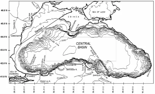
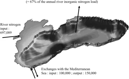
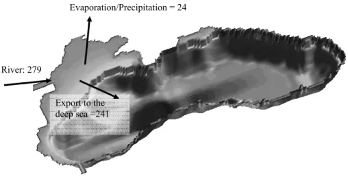
The Black Sea is by large an elliptical basin with an area of 423 000 km2 and a vol-ume of 534 000 km3which has only restricted exchanges with the Mediterranean Sea through the narrow Bosphorus strait (Fig. 1). This marine area exhibits topographic and hydrographic specificities which make it interesting for testing models and pro-25

cesses. It presents a large variety of topography with a flat abyssal plain (maximum depth 2200 m) in the central part and an almost 200 km wide shelf in the north-western area (depth <100 m, constituting 25% of the total area). The northwestern shelf forms a shallow receptacle for the most important Black Sea rivers (i.e. the Danube, the Dnestr

(5)

BGD

1, 107–166, 2004

Full Screen / Esc

and the Dnepr), and is well known to be a region of enhanced biological production fed by the nutrients brought by the river discharges, as shown by satellite images (e.g. Sur et al., 1994; Nezlin et al., 1999). The landlocked geometry of the Black Sea basin makes easier the computation of water and nitrogen budgets to check the internal con-sistency of the model dynamics and the convergence towards a steady state solution. 5

The Black Sea is a typical example of estuarine basin and therefore, its overall mass budget and hydrochemical structure critically depend on elements of the hydrological balance. Its hydrographic regime is characterized by low salinity surface waters of river origin overlying high-salinity deep waters of Mediterranean origin. As a result, a permanent pycnocline (or more precisely a halocline) develops with a depth vary-10

ing horizontally according to the local hydrodynamics between 100–150 m and inhibits the exchanges between the surface and deep waters. These conditions have made the Black Sea almost completely anoxic with oxygen only in the upper 150 m depth (13% of the sea volume) and hydrogen sulfide and methane in the deep waters. The atmospheric forcings only affect the surface layer and cold intermediate waters and, 15

therefore, waters below 500 m depth are essentially stagnant. The residence time in-creases from a few years for the layer of the main pycnocline (e.g. Unluata et al., 1990; Buesseler et al., 1991) to a few thousands of years for the deepest layer (e.g. Ozsoy and Unluata, 1997).

The above specific features give enough arguments to consider the Black Sea as a 20

natural test area for modeling studies where the different factors leading to the degra-dation of its ecosystem can be identified and analyzed. Most of the mathematical models applied to the Black Sea to study the functioning of its ecosystem are limited to interaction box models (e.g. Cokacar and Ozsoy, 1998; Ozsoy et al., 1998) or to one-dimensional (vertical) coupled physical biogeochemical models usually describing 25

the nitrogen cycling (e.g. Lebedeva and Shushkina, 1994; Oguz et al., 1996, 1999; Staneva et al., 1998; Lancelot et al., 2002). Models applied in the suboxic zone and describing the nitrogen and sulfur cycles coupled with oxygen dynamics (e.g. Yakushev and Neretin, 1997; Oguz et al., 1998) and also, to the manganese cycle (e.g. Yakushev,

(6)

BGD

1, 107–166, 2004

Full Screen / Esc

1998; Oguz et al., 2000) have also been developed.

The model presented in this paper is used with the aim of understanding the macroscale (i.e. time scales of a few weeks to months) Black Sea’s ecohydrodynamics and more specifically: (1) to estimate the transport at the shelf break of water, biogenic nutrients and plankton (2) to understand, quantify and compare the nitrogen cycling of 5

the north-western shelf and of the deep sea, (3) to quantify the vertical flux of nitrate and PON at different depths of the central basin as well as its seasonal variability, (4) to estimate the free nitrogen production due to the denitrification process occurring in oxygen-deficient waters and (5) to quantify the role of the Black Sea basin in the carbon exportation and sequestration (the efficiency of the biological pump) in the deep layers. 10

The paper is organized as follows. Section 2 briefly describes the coupled model and its convergence towards a steady state solution as well as the numerical scheme used to discretize the evolution equations of the biogeochemical components. Model results are described in Sect. 3. First, the main characteristics of the Black Sea’s macroscale ecohydrodynamics simulated by the model are illustrated. Then, the sea-15

sonal variability of the water and nutrients transports at the shelf break is analyzed and the nitrogen budgets of the whole basin, the north-western shelf and the central basin are quantified. Finally, a discussion and conclusions are presented in Sect. 4.

2. The mathematical tool: description of the three-dimensional model

The three-dimensional model results from the on-line coupling between a general cir-20

culation model and an ecosystem model.

2.1. The hydrodynamical model

The macroscale hydrodynamics of the Black Sea has been numerically simulated with the GHER general circulation model covering the whole basin (27.15◦E– 42.64◦E×40.61◦N–46.68◦N). The GHER primitive equation model is derived from the 25

(7)

BGD

1, 107–166, 2004

Full Screen / Esc

general “marine weather” model by averaging over a time scale of several weeks. This model is three-dimensional, non linear, baroclinic and solves for the free surface, the three components of the current field, temperature, salinity and turbulent kinetic en-ergy. Being an estuarine basin, the Black sea is very sensitive to variations in the fresh water balance. The resulting free surface movements are of utmost importance 5

for establishing the circulation, and therefore the use of a free surface model allows to more adequately describe the variations of the sea surface elevation induced by river runoff (Stanev and Beckers, 1999). The model uses a refined turbulent closure scheme defined by the turbulent kinetic energy and a mixing length which is calculated alge-braically from a parametric neutral mixing length formulation modified by stratification 10

effects. The density field is computed from the model temperature and salinity fields using a standard state equation for the sea water. Subgrid scale processes are param-eterized by a laplacian operator with a horizontal diffusion coefficients of 500 m2s−1for momentum and 50 m2s−1for scalars. The GHER general circulation model has been successfully applied to explore the general circulation of the Bering Sea (e.g. Deleer-15

snijder and Nihoul, 1988), the Mediterranean Sea (e.g. Beckers, 1991), the North Sea (e.g. Delhez, 1996), and, more recently, the Black Sea (e.g. Gr ´egoire, 1998a; Gr ´egoire et al., 1998b, 2004; Stanev and Beckers, 1999; Beckers et al., 2001).

2.2. The ecosystem model

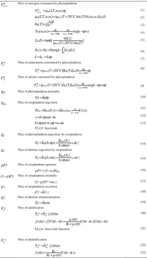
The biogeochemical model describes the nitrogen cycling through the pelagic foodweb 20

(all the biogeochemical state variables are expressed in mmol N m−3 except benthic detritus which are expressed in mmol N m−2) and its state variables are defined ac-cording to the recommendations of the GLOBEC Numerical Modeling group as those which are thought to be necessary and sufficient to characterize the main features of the ecosystem response to a 3D environment at seasonal scales (GLOBEC, 1997). It is 25

described by a 6 aggregated variables defined on the base of the functional role played in the trophic dynamics by planktonic populations: the phytoplankton and zooplankton biomass without reference to species, total pelagic detritus (lumping together dissolved

(8)

BGD

1, 107–166, 2004

Full Screen / Esc

and particulate dead organic matter), nitrate, ammonium and benthic detritus. The phy-toplankton (ϕ) represents all the primary producers. All the heterotrophs with a size ranging between 2 µm and 2 mm are described by the zooplankton compartment (z). The dead organic matter (particulate and dissolved) (ω) is described by the detritus compartment. Since the microbial loop of the Black Sea’s oxygenated waters is partic-5

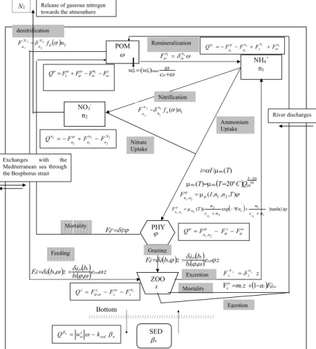
ularly efficient (e.g. Sorokin, 1983; Karl and Knauer, 1991), the bacterioplankton has been eliminated from the model assuming quasi-equilibrium, prey-predator relation-ships within the microbial loop. Also, particulate organic material is directly converted to ammonium. Finally, the sediments are described by the benthic nitrogen pool β_n.

A schematic representation of the ecosystem model with all the interaction terms 10

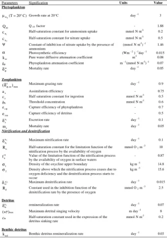
written on the arrows is given in Fig. 2. The evolution equations of the biogeochem-ical state variables and the mathematbiogeochem-ical formulation of the biogeochembiogeochem-ical interac-tions are described in extenso in Gr ´egoire (1998a) and Gr ´egoire et al. (2004) and are summarized in the Appendix 1. The initial and boundary conditions used to force the hydrodynamical and biogeochemical models are described in the Appendix 2.

15

The estimation of biogeochemical parameters is based on available observations and studies (e.g. Oguz et al., 1996, 1998; Ozsoy et al., 1998) realized in the Black Sea or in other similar environments such as the Baltic Sea and the North Sea. Since, in a 3 D frame, one year of integration takes about 3 days of computation, some preliminary sensitivity studies are made with a box version of the model to determine the key 20

parameters on the outcome of the ecosystem model (e.g. the sedimentation velocity, the maximum grazing rate). Once these parameters are known, the calibration of the 3D model consists essentially in adjusting them by a series of sensitivity experiments until the simulations show a good agreement with the available observations set.

2.3. Implementation of the model 25

The mathematical model offers a 3D view of the marine system and is formulated in the so-called σ-coordinate system to follow the bathymetry as closely as possible and to avoid the rigid lid approximation for the motions of the free surface (a

(9)

two-BGD

1, 107–166, 2004

Full Screen / Esc

fold σt coordinate system is used in regions of large bathymetric variations and of large depths). The numerical resolution is achieved through the 3D-finite differencing method on an Arakawa C-grid. To simulate the general circulation and associated synoptic structures, the domain is covered with a 15×15 km horizontal numerical grid and 25 vertical σ-layers. The model marginally solves the rossby radius of deformation 5

in the Black Sea which is about 20 km. The spacing of the vertical layers is adjusted to offer a finer resolution in the vicinity of the surface and of the thermocline (the thickness of the vertical layers is about 5 m in the upper 30 m and 10 m down to 100 m).

A centered-space differencing scheme is used to discretize the horizontal and ver-tical diffusion terms while an hybrid scheme, combining a centered and a streamline 10

upwind discretization scheme is used for the advection (horizontal and vertical) terms. An explicit time step scheme is used to discretize horizontal fluxes while an implicit scheme is used on the vertical avoiding computational instabilities which may arise due to the use of a fine vertical resolution in the surface and bottom layers. The mode splitting technique is used to solve the equations of the rapidly evolving sur-15

face gravity waves (Madala and Piacsek, 1977). The resolution of a particular equation is done using the most recent value for each variable. The discretization of the produc-tion/destruction term of each biological state variable is based on a Patankar technique (Patankar, 1980). An explicit scheme is used for the production term while the destruc-tion term is linearly implicitly discretized. Then, disregarding the denitrificadestruc-tion term 20

which represents a definitive nitrogen loss for the system, the sum of all the biogeo-chemical interaction terms is not strictly equal to zero as it should be if the system was fully numerically conservative. With a totally explicit numerical scheme, the sum of all the biogeochemical interaction terms would be exactly zero after discretization. How-ever, an explicit scheme is completely instable whatever is the time step of integration. 25

To reduce the artificial production/destruction of matter, the dominant biological fluxes (i.e. the phytoplankton growth rate, the grazing rate) have to be computed at a given time-step consistently and therefore, the sequence of integration of the biogeochemical equations corresponds to the sense of the flux of matter in the ecosystem (i.e. inorganic

(10)

BGD

1, 107–166, 2004

Full Screen / Esc

nitrogen, phytoplankton, zooplankton, detritus). To quantify the conservation properly of the numerical scheme used in this study, one computes the evolution of the sum of the biogeochemical interaction terms (disregarding the denitrification term). It has been found that with a time step of 1 h, the annual mean value of this sum is at maxi-mum by two to three orders of magnitude lower than the typical value of the interaction 5

terms. The maximum values are found in regions particularly active from a biological point of view and characterized by rapid fluctuations in the biogeochemical constituents on time scales comparable to the time step of integration (e.g. the Danube’s discharge area, the western coast). Also, integrated over the whole basin and year, this artificial creation/destruction of matter due to the non-perfect numerically conservativity of the 10

model was estimated to represent 1.3% of the order of magnitude of annual basin-wide integrated biogeochemical fluxes.

2.4. Transient adjustment

After ten years of integration of the physical model, the amplitude of the seasonal cycle is more or less established in response to the imposed external forcings and to the 15

internal processes in the system. During the 10-year spin-up, the annual mean vertical stratification does not show substantial trends and remains close to the initial data. Af-ter this spin-up time, the hydrodynamical model is in balance and the basin inventory of water and salt remain constant over the annual cycle (Stanev and Beckers, 1999). This does not mean that trends are totally absent but, at the scale of our study (i.e. the 20

seasonal cycle), the small trends, which may be potentially important for paleoceanog-raphy, could not significantly affect the results of the model. Using the results of the tenth year of integration of the physical model, the biological model of the upper layer ecosystem is then integrated to obtain almost repetitive yearly cycles of the biological variables (this is the case after three years of integration).

25

The quantitative measure of testing the attainment of the cyclical state is to check whether the 3D integrated (i.e. over the two horizontal directions and over the vertical) total nitrogen content, N (=n+n+ϕ+ z + ω + β) is approaching to a constant value

(11)

BGD

1, 107–166, 2004

Full Screen / Esc

over the annual cycle. This requires a perfect equilibrium between the nitrogen sources (i.e. the rivers and the Mediterranean inputs) and sinks (i.e. the denitrification, the ex-port towards the anoxic layer and Mediterranean Sea). Since the river inputs and the Mediterranean exchanges are almost entirely imposed from the data (in the Bosphorus Strait, nutrients profiles measured in-situ are imposed, see Appendix 2; for the water 5

fluxes, the fluxes give a water budget in equilibrium), the obtainment of an equilibrium solution will depend essentially on the ability of the model to represent adequately the amplitude of denitrification and sedimentation towards the deep waters. However, it is well known from sediment trap analysis and modeling studies that the amount of organic matter sedimenting towards the deep basin represents only a few percents of 10

the amount of organic matter produced by photosynthesis (e.g. Karl and Knauer, 1991; Oguz et al., 1999; Gr ´egoire and Lacroix, 2003). Therefore, to reach a steady state, the modelled denitrification process occurring in the water column should be able to elim-inate a high percentage of the huge river nitrogen inputs. Figure 3 gives the different terms of the model estimated basin wide integrated annual nitrogen budget (in t N yr−1). 15

The basin wide nitrogen budget established from model results is not in equilibrium The nitrogen content of the whole basin (mainly the nitrate content) increases by 3% each year of integration. Figure 3 shows that the denitrification process constitutes the pri-mary loss of nitrogen in the Black Sea with an estimated annual loss of free nitrogen of about 4.5×105t. Therefore, 67% of the total annual load of inorganic nitrogen brought 20

into the shelf by the rivers is irreversibly lost by denitrification (the annual load of inor-ganic nitrogen brought by the rivers equals 671,169). This last value is lower than the estimation of 75% made by Konovalov et al. (2000) with a budget model. Integrating over the whole basin the results of a 1D model, Yakushev and Neretin (1997) estimated to 106t the annual amount of free nitrogen produced by denitrification. Thus, the model 25

seems to underestimate the basin wide free nitrogen production due to denitrification as a result of the incapacity of the foodweb represented by the model to assimilate all the nitrate discharged by the rivers (this point will be clarify in Sect. 3.2). However, it should be noted that, on the one hand, the calculation of free nitrogen production in the

(12)

BGD

1, 107–166, 2004

Full Screen / Esc

model does not account for nitrogen production during thiodenitrification because the contribution of this process is assumed to be negligible when compared with nitrogen production during denitrification (e.g. Yakushev and Neretin, 1997). On the other hand, it is clear that the amount of nitrogen eliminated by denitrification is strongly linked to the input of inorganic nitrogen by the rivers. The model considers that every year the 5

rivers introduce 617×103t of inorganic nitrogen. This value lies in the lower range of the observed estimates which are between 600×103t and 106t. We do not know for which value of the river discharge, Yakushev and Neretin (1997) estimated the Black Sea free nitrogen production to 106t. Therefore, we can suspect that the increase of the nitrate content after each year of integration is due to the incapacity of the ecosys-10

tem model to incorporate the totality of the river nitrate input in the upper layer organic matter cycle. Most of this unconsumed nitrate accumulates in the surface layer and does not reach the transitional layer to be eliminated by denitrification. It should also be noted that the increase of the nitrate inventory can be due to the non representation of the denitrification process as a process of benthic remineralization on the shelf. In 15

the model, PON reaching the shelf sediments is totally remineralized. No burial and denitrification have been represented. In Gregoire and Friedrich (2004), it has been found that benthic denitrification occurring on the shelf sediments may be an important pathway of nitrogen elimination in the Black Sea. Integrating over the whole shelf and year, some punctual measurements obtained in summer 1995 and spring 1997 in the 20

framework of the EU EROS 21 project, they obtained that about 60% of the PON flux reaching the shelf sediment may be eliminated by denitrification against about 8–17% for burial. With these values, about 50% of the annual load of inorganic nitrogen dis-charged by the Danube is lost through denitrification and burial. Although these last values can be criticized because they are obtained by integrating over the whole shelf 25

and year some punctual measurements realized during a few weeks, they suggest that benthic denitrification is important.

(13)

BGD

1, 107–166, 2004

Full Screen / Esc

3. Model results and discussion

3.1. The hydrodynamics

A detailed description of the Black Sea’s hydrodynamics simulated by the model is given in Gr ´egoire (1998a), Gr ´egoire et al. (1998b) and Stanev and Beckers (1999). Here the main characteristics of the general circulation and of the frontal system are 5

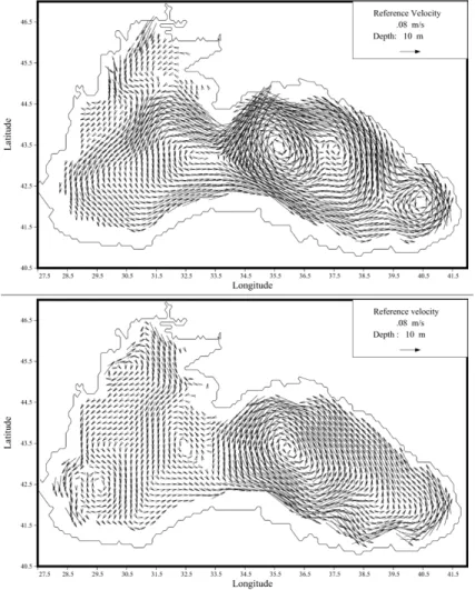
described stressing the aspects of the hydrodynamics that may affect the ecodynamics. A basin scale, coherent, cyclonic boundary current is the main feature of the Black Sea general circulation (e.g. Stanev, 1990; Oguz et al., 1992, 1993; Stanev and Beck-ers, 1999). This cyclonic circulation results essentially of the cyclonic wind pattern (positive curl of wind stress) but is also driven by the large scale hydro-thermodynamic 10

forcing (surface and lateral buoyancy) and is controlled by the topography (e.g. Stanev, 1990). The mean position of the main surface current coincides approximately with the position of the continental slope, but important deviations are observed due to eddy variability, direct impact of atmospheric forcing or interannual variability. This cyclonic type of circulation dominates the vector plots of Fig. 4, but shows pronounced seasonal 15

dependency, which is important for the transport of plankton and other biogeochemical components.

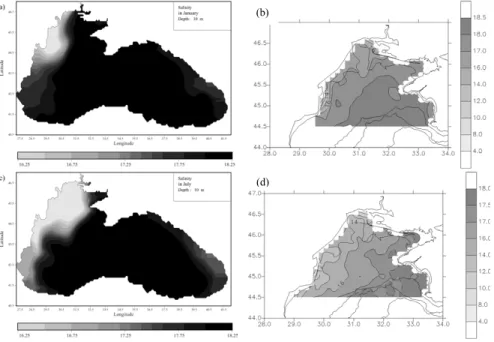
The shallow north-western shelf constitutes the coldest part of the Black Sea throughout the year (e.g. Ozsoy and Unluata, 1997; Ginzburg et al., 2001) and re-ceives the fresh water inputs of the Danube, Dnestr and Dnepr rivers. This leads to 20

the formation of a strong haline front which can be observed during the whole year with seasonal modifications in its intensity and structure resulting mainly from the pro-nounced seasonal variability of the north-western shelf circulation (Fig. 5). This strong haline front confines river waters along the western coast and prevents the mixing be-tween the coastal waters and the more saline open sea waters characterized by a 25

salinity of ≈18–18.2.

The circulation in the central and eastern parts of the sea remains relatively stable during the year, and the patterns do not show reversals of the current. On the contrary,

(14)

BGD

1, 107–166, 2004

Full Screen / Esc

the variability of the circulation is very pronounced between the main gyre and the coast, and in particular, on the north-western shelf. This variability is illustrated by the presence of semi-permanent eddies, by the ejection of filaments generated by baroclinic instabilities at the frontal interface and by the reversal of the surface current of the north-western shelf at the end of spring until the end of fall. This reversal of the 5

flow has an important impact on the distribution of the primary production of the area because it transports the rich nutrient Danube’s water towards the north-eastern part of the shelf (e.g. Gr ´egoire et al., 2004). This north-east extension of the low salinity river waters on the shelf at the end of spring has also been revealed by in-situ data (Fig. 5).

10

3.2. The ecodynamics

Both model results and observations illustrate a highly complex spatial variability of the phytoplankton annual cycle imparted by the horizontal and vertical variations of the physical and chemical properties of the water column. The frontal interface separating river waters and open sea waters is primarily a boundary between the eutrophic shelf 15

waters and the less productive open sea waters. On the north-western shelf, the model shows that the seasonal evolution of the productive waters illustrated by the satellite images is primarily connected to the seasonal variation of the north-western shelf cir-culation that leads to modification in the transport of the rich nutrients Danube’s waters. In all the regions, the phytoplankton annual cycle is characterized by the presence of a 20

winter-early spring bloom. This bloom precedes the onset of the seasonal thermocline and occurs as soon as the mixing layer depth reduces and becomes comparable or shallower than the euphotic layer depth. In the Danube’s discharge area and along the western coast, where surface waters are almost continuously enriched in river nutrient, the phytoplankton development is sustained during the whole year at the surface with 25

seasonal modifications in its intensity. On the contrary, in the central basin, the primary production in the surface layer relies essentially on nutrients being entrained in the up-per layer from below and a winter-early spring bloom is simulated in agreement with

(15)

BGD

1, 107–166, 2004

Full Screen / Esc

field observations. At the end of spring and in summer, the maximum development of the phytoplankton is observed at depth, below the thermocline, except at the Danube’s mouth where it occurs at the surface all over the year.

The qualitative comparison of model results with SeaWiFS satellite data shows that the model reproduces reasonably well the space-time evolution of the phytoplankton 5

distribution. On a quantitative point of view, however, the model underestimates the phytoplankton biomass in the Danube’s discharge area and along the western coast. In these regions, the extremely high nutrient concentrations allows the phytoplankton growth at almost nutrients saturation conditions. However, as soon as the simulated phytoplankton biomass reaches a threshold value, the zooplankton develops and main-10

tains a strong control on the phytoplankton development. This deficiency is typical of simple ecosystem models considering only one phytoplankton and one zooplankton compartment which may overestimate the grazing pressure. Similar conclusions have been found earlier by Sarmiento et al. (1993) in their North Atlantic model, and by Oguz et al. (1999) in their Black Sea model.

15

The plankton annual cycle simultaed by the model is described in extenso in Gre-goire (1998b) and GreGre-goire et al. (2004) and is compared with satellite and in-situ observations.

3.3. Primary production

The Black Sea is known as a region of moderate to high biological productivity: the 20

north-western shelf into which the major Black Sea’s rivers flow is characterized by the highest productivity while the central basin, where the biological production re-lies essentially on nutrients being entrained from below by the vertical mixing, is a region of moderate productivity. Using an algal carbon to nitrogen ratio of ∼8.5 for nitrogen limited ecosystem, the model estimates to 130 g C m−2yr−1 the vertically in-25

tegrated primary production of the whole basin which is lower than the estimates of 200 g C m−2yr−1made by Sorokin (1983).

(16)

BGD

1, 107–166, 2004

Full Screen / Esc

3.3.1. Primary production of the central basin

The vertically integrated annual primary production estimate of 40 g C m−2yr−1 from the model lies in the lower values of the observed estimates which are between 40 g C m−2yr−1 (Finenko, 1979) and 90 g C m−2yr−1 (Sorokin, 1983) from the various measurements in the central part of the sea. The model estimate is about the third of 5

the estimate of 150 g C m−2yr−1 made by Vedernikov and Demidov (1993). However, according to Oguz et al. (1999), this last value is misleading, since it is based on a multi-year composite data set, which includes more than one set of late winter-early spring bloom events that occurred on different days in different years and therefore these measurements may overestimate the annual primary production rate.

10

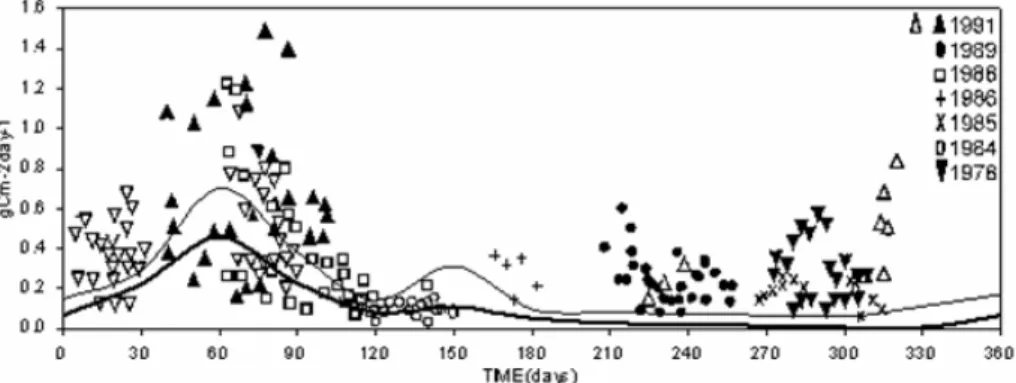
The annual cycles of the vertically integrated primary production produced by the model for the whole central basin and for the region of the eastern main cyclonic gyre (mean spatial profiles) are compared with the values of a series of measurements made between 1978–1991 and reported by Vedernikov and Demidov (1993) (Fig. 6). The highest values of 0.7 g C m−2d−1 and 0.45 g C m−2d−1 for respectively the east-15

ern gyre and the whole central area are simulated in winter-early spring (February-March) when the vertical flux of inorganic nutrients through the euphotic layer reaches its maximum (see Fig. 14). These values compare reasonably well with the in-situ mea-surements of 0.2–1.5 g C m−2d−1made by Vedernikov and Demidov (1993) (Fig. 6) as well as with the observations of 0.2–0.96 g C m−2d−1 (mean 0.4 g C m−2d−1) realized 20

by Mikaelyan (1995) at different stations of the central basin for the period February– March 1991. Model results show that the primary production is at maximum in the cen-ters of the main cyclonic gyres of the central basin and decreases towards the periph-ery. The winter-early spring bloom is followed by a secondary peak in late spring (May– June) with values between 0.31 g C m−2d−1 for the eastern gyre and 0.11 g C m−2d−1 25

for the whole central basin. These values are in agreement with typical measurements for this period which are of 0.1–0.6 g C m−2d−1 (Vedernikov and Demidov, 1993) and 0.3–0.5 g C m−2d−1 in the center of the western main cyclonic gyre in May 1988 (Karl

(17)

BGD

1, 107–166, 2004

Full Screen / Esc

and Knauer, 1991). The summer-early fall period is found to be the less productive period characterized by values less than 0.1 g C m−2d−1 (about 0.07 g C m−2d−1 for the eastern gyre and 0.02 g C m−2d−1for the whole central basin) whereas the obser-vations values vary from 0.2 to 0.6 g C m−2d−1 in the same period (Vedernikov and Demidov, 1993). These recent estimations are much higher than the 1960’s observa-5

tions (Sorokin, 1983) which gave values between 0.05 g C m−2d−1and 0.5 g C m−2d−1 for the different stations within the central Black Sea. It is reported that the primary production in the central part of the sea has increased by a factor of 3 to 4 over the last 30 years (Sorokin, 1964; Stelmakh et al., 1998). The underestimation of the primary production in early fall by the model is likely due to the underestimation of the vertical 10

mixing at this period. This period is characterized by the presence of weekly storms which are not adequately represented in the model although they are expected to en-hance temporarily the upward flux of nitrate into the surface layer (Oguz et al, 1996). Indeed, since the model is forced at the air-sea interface by the mean wind stress at macroscale produced by a monthly mean wind and not, as it should be, by the mean 15

wind stress including a quite significant component due to non-linear interactions of mesoscale winds, small scales events such as storms are not well represented and this leads to an underestimation of the production of turbulent kinetic energy at the surface. On the other hand, at the surface, temperatures values are relaxed towards climatological monthly mean values and this leads to an overestimation of surface tem-20

peratures. Therefore, the vertical mixing by convection is underestimated. Besides, it should be noted that using a relaxation scheme for the temperature to force the model at the surface instead of the heat fluxes underestimates the vertical penetration of the seasonal atmospheric signal. For instance, in spring, only the first upper 15 m are af-fected by the seasonal heating of the water column. As a result, in summer, the vertical 25

extension of the thermocline is estimated to about 13 m while field observations give a vertical extension of about 30 m. Also, the early-fall peak in primary production is delayed and only occurs in November-December when the intensification of the wind stress destroys the seasonal thermocline of the central basin. In November, the

(18)

pri-BGD

1, 107–166, 2004

Full Screen / Esc

mary production increases and reaches in December 0.2 g C m−2d−1 in the center of the eastern main cyclonic gyre which is slightly lower that the values of 0.36 g C m−2d−1 obtained as an average of measurements from all stations in the central basin at the time of the autumn bloom (Vedernikov and Demidov, 1993).

3.3.2. Primary production of the north-western shelf 5

The model estimated vertically integrated annual primary production of 220 g C m−2yr−1 is in good agreement with the measurements of Sorokin (1983) which gave a value of 250 g C m−2yr−1. These last values are much higher than the total primary production of the Gulf of Lions in the Mediterranean Sea fed by the nutrients input of the Rhone river (annual nitrate input =70 000 t, about a tenth of 10

the Danube’s input) which is estimated between 77 g C m−2yr−1 and 106 g C m−2yr−1 (Tusseau et al., 1998).

Our model estimates of the annual primary production of the shelf and of the cen-tral basin are in good agreement with the observations made for different regions of the world by Ryther (1969) which give values of 50 g C m−2yr−1 for oceanic waters, 15

100 g C m−2yr−1 for coastal and neritic regions and 300 g C m−2yr−1 for upwelled wa-ters.

3.4. Water and nitrogen exchanges between the north-western continental shelf and the deep sea

The model allows us to quantify the monthly integrated fluxes of water and of any bio-20

geochemical component at the shelf break represented by the vertical section shown in Fig. 1 (Sect. 1, surface 50 km2). The area located at the north of this section is char-acterized by a depth lower than 150 m and is considered representative for the Black Sea’s north western shelf (volume: 4,7×103km3, surface: 50×103km2).

(19)

BGD

1, 107–166, 2004

Full Screen / Esc

3.5. Water transport fluxes

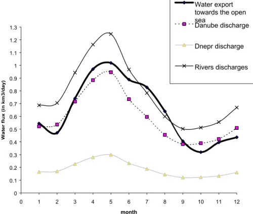
The seasonal variations of the net water transport flux follow the annual cycle of the river discharges with a peak in May and a minimum in October when the river dis-charges reach respectively their maximum and minimum values (Fig. 7). Figure 8 displaying the different terms of the north-western shelf annual water budget shows 5

that the global budget (which would be equal to zero if no error was made when diag-nostically computing the water export through Sect. 1 is equal to 14 km3and therefore, one estimates the relative error associated to the computation of the water export to about 6%.

The space-time variability of the water transport flux through the shelf break is ex-10

tremely high. For instance, the comparison of Figs. 9a and 9b illustrating respectively the vertical distribution through Sect. 1 of the annual mean water flux and of its stan-dard deviation (showing the seasonal variability in the water transport flux) indicates that the standard deviation is comparable to the annual mean and is particularly high in the eastern part of the section due to the pronounced variability of the circulation in 15

this area (Fig. 4). Indeed, from the end of spring until the end of fall, the circulation on the shelf is anticyclonic and a strong flux of water leaves the shelf in the eastern part while, in winter, the surface current reverses and becomes cyclonic and surface waters are transported onto the shelf from the open sea (Figs. 9c and 9d). In addi-tion to this pronounced temporal variability, the spatial variability is also very high. The 20

flux of water leaving the shelf is mainly concentrated in the upper 50 m while below, the water flux usually enters into the shelf. The spatial mean of the normal velocity to Sect. 1 is estimated to −0.163×10−3m/s (spatial mean value of the annual mean velocity field normal to Sect. 1) and is an order of magnitude lower than its standard deviation (showing the spatial variability in the water transport flux) of 0.5046×10−2. 25

Therefore, considering this pronounced variability, the error made on the water export calculation is totally acceptable.

(20)

BGD

1, 107–166, 2004

Full Screen / Esc

3.5.1. Nitrogen transport fluxes

The annual cycle of the net nitrogen transport across the shelf break presents two peaks (Fig. 10). The first one, in April-May, is associated whth the major peak in the river discharges. The second one occurs in September and is not observed in the water transport flux (Fig. 7). This last peak occurs when the rich nitrate Danube’s 5

waters transported from the river’s mouth by the anticyclonic shelf current reach the shelf break and penetrate into the western part of the central basin (Fig. 11e). As one can expect, the transport by diffusion is usually lower than the advection transport especially during the second half of the year when the diffusion transport is almost by one order of magnitude lower than the advection flux (Figs. 11c and 11d). Also, 10

the annual cycle of the total nitrogen transport follows approximately the cycle of the advection flux but is higher. Of course, the nitrogen transport is essentially determined by the nitrate transport. The net integrated (over the whole vertical section) advection and diffusion transports are both positive during the whole year (Fig. 10) because, on the one hand, the integrated water transport is also positive throughout the year and, 15

on the other hand, the nitrogen concentrations of the shelf waters are much higher than in the open sea. The model shows that the annual nitrogen net loss for the shelf above 55 m reaches 610 040 t. As for the water transport, the space-time variability of the nitrogen transport flux is highly pronounced. The spatial mean of the annual mean nitrogen transport is −0.4044×10−1mmol N m−2s−1and the standard deviation equals 20

0.102. This variability is essentially communicated by the advection flux which has a spatial mean of −0.2601×10−1mmol N m−2s−1and a standard deviation of 0.98×10−1 while the diffusion flux has a mean of −0.144×10−1mmol N m−2s−1 and a standard deviation of 0.811×10−2.

This strong spatial and temporal variability of the nitrogen and water transport can be 25

explained by the 3D complexity of the circulation along the shelf break. The variability of the north-western shelf circulation is mainly illustrated by the reversal of the surface current at the end of spring until the end of fall and the generation, at the Danube’s

(21)

BGD

1, 107–166, 2004

Full Screen / Esc

mouth, of an anticyclonic eddy with a length scale of some tens of km (Fig. 4). Also, this suggests that it would be extremely delicate to apply a high resolution model to the shelf forced at the open sea by boundary fluxes computed by a coarse resolution model applied to the whole basin.

3.6. Nitrogen cycling on the north-western shelf 5

The amount of nitrogen transferred by biogeochemical processes between the different modeled compartments has been quantified as well as the evolution over one year of integration of the nitrogen content of each compartment (results representative of the situation reached after five years of integration) (Fig. 12). The annual nitrogen budget of the north-western shelf implies an approximate balance between the variation of 10

the nitrogen inventory of the shelf, the external input of total nitrogen by the rivers and the nitrogen transported at the shelf break. This balance is almost verified and one estimates the relative error on the diagnostic computation of the nitrogen export towards the open sea to about 5.6% which is in agreement with the estimated relative error on the water export.

15

The biological fluxes almost compensate each other and are the dominant terms of the nitrogen budget of each biogeochemical state variable. Indeed, the biological fluxes integrated over one year are at least by one order of magnitude (except for ni-trate and benthic detritus) greater than the river discharges, the transport at the shelf break and than the nitrogen content of the biogeochemical compartment. This implies 20

a short turnover time (from a few days to a hundredth of days for nitrate) for these com-partments and thus, the possibility of fast changes in their nitrogen inventory caused by small changes in the rate of biogeochemical processes and also in the river discharges and the exchanges at the open sea. Therefore, the variation of the nitrogen content of each biogeochemical state variable after one year of integration, which is at maximum 25

of 10% (for the nitrate), lies within the error bars of the biogeochemical model (asso-ciated to the non-fully conservative numerical discretization, see Sect. 2.3) and of the computed export.

(22)

BGD

1, 107–166, 2004

Full Screen / Esc

The dominant biogeochemical fluxes are the nutrient uptake by phytoplankton, the grazing, the remineralization, the nitrification and the excretion. The loss of nitrogen by denitrification equals zero. The fluxes towards and from the sediments almost compen-sate and are at least by one order of magnitude lower than the other biogeochemical fluxes.

5

The budget indicates that the total primary production of the shelf (800×103t N yr−1+726×103t N yr−1=1,526×103t N yr−1) and the export of inorganic nitrogen towards the deep sea (763×103t N yr−1) are roughly compensated by the ammonium regenerated through the remineralization of detritus in the water column (598×103t N yr−1) and in the sediments (174×103t N yr−1) and through zooplankton 10

excretion (683×103t N yr−1) plus the external input of total inorganic nitrogen into the shelf by the rivers (671×103t N yr−1). The recycling of organic matter in the water column through zooplankton excretion and detritus remineralization represents 84% of the total primary production, benthic recycling represents 11.4% of the total primary production and the river inorganic nitrogen discharge 44%. 36% of the annual load 15

of inorganic nitrogen brought by the rivers and remineralized in-situ is not consumed by the primary producers and is exported towards the deep sea. The nitrate and ammonium uptakes are respectively 800×103t N yr−1 and 726×103t N yr−1 which accounts 52.4% and 47.6% of the annual total primary production.

The comparison of the flux of PON and ammonium respectively to and from the 20

sediments obtained by the model and in-situ observations collected during the EU EROS-21 and INTAS project is described in extenso in Gregoire and Friedrich (2004).

3.7. Nitrogen cycling in the central basin

3.7.1. Nitrogen budget of the euphotic layer of the central basin

The nitrogen budget of the euphotic layer of the central basin (volume=6×103km3, 25

surface=110×103km2) has been computed to provide the intercompartmental transfer rates and the fluxes across the base of the euphotic layer (Fig. 13). Since the

(23)

deni-BGD

1, 107–166, 2004

Full Screen / Esc

trification process does not occur in the euphotic layer, a perfect steady state solution implies an approximate balance between the external input of total nitrogen into the euphotic layer by horizontal and vertical physical fluxes. However, this balance is not strictly verified (the annual net vertical nitrogen flux at the base of the euphotic layer is an upward flux of 7×103t and the net horizontal flux represents also a gain of nitrogen 5

for the central basin with a value of 5×103t) and therefore, the nitrogen content of the euphotic layer increases by 21×103t after one year of integration. This unbalance can also be explained by the existence of a possible error made when computing the net horizontal/vertical physical fluxes through the boundaries of the domain of integration since these fluxes are characterized by a pronounced spatial variability. Indeed, their 10

standard deviation is comparable or by one order of magnitude higher than their spatial mean. It implies a strong sensitivity of the results to the size of the domain of integra-tion. This pronounced variability can be explain by the high variability of the circulation between the coast and the main cyclonic gyres of the central basin and also around the shelf break. On the other hand, the annual nitrogen budget of each compartment 15

is almost satisfied with an estimated relative error of less than 10% on the different physical/biogeochemical fluxes.

The vertical and horizontal physical fluxes of each biogeochemical compartment are about of the same order of magnitude except for the detritus for which the vertical flux is about 20 times higher due to the sedimentation process. However, the hor-20

izontal fluxes of each compartment roughly compensate and, when computing the budget of each biogeochemical compartment, the vertical flux of nitrate, ammonium and detritus is by about one order of magnitude higher than the net horizontal flux. The biogeochemical interaction terms are by one order of magnitude higher than the physical terms except for the detritus and nitrate. The low ratio of the nitrogen stock 25

of each biological compartment to the biogeochemical/physical (vertical/horizontal ad-vection/diffusion) in/outflux means that the residence time (the time necessary for the biological and physical fluxes to replace the whole stock of nitrogen of the euphotic layer) of the nitrogen content of these compartments in the euphotic layer is fairly short

(24)

BGD

1, 107–166, 2004

Full Screen / Esc

(from about half a year for the nitrate to a few days for the other compartments). The nitrate and ammonium uptakes are respectively 402×103t N yr−1 and 216×103t N yr−1 which accounts 65% and 35% of the total annual primary production (619×103t N yr−1). This production is compensated by the ammonium regenerated within the euphotic zone through the remineralization of detritus (318×103t N yr−1) and 5

zooplankton excretion (71×103t N yr−1) plus the external input of total inorganic nitro-gen into the euphotic zone by horizontal and vertical advection/diffusion (respectively 24×103t N yr−1and 207×103t N yr−1). These last values stress the efficiency of the in-situ regeneration process which provides over the year to the euphotic layer 389×103t of inorganic nitrogen against 231×103t for the physical processes. These values sug-10

gest also that the recycled production primarily occurs through the detrital pool rather than immediate zooplankton excretion. However, this can also result from the weak zooplankton development in the central basin due to the existence in the grazing func-tion used in the model of a threshold concentrafunc-tion (i.e. 0.6 mmol N m−3) below which the zooplankton does not develop (see the model description in the Appendix 1). This 15

threshold takes into account a well-known behavior of the zooplankton which consists of stopping its feeding activity when the energy gained from the feeding of its preys is lower than the energy spent for capturing them (e.g. Mullin, 1963; Andersen and Nival, 1988).

3.7.2. Vertical flux of inorganic nitrogen: seasonal evolution and vertical profile 20

The annual mean vertical profile of the total vertical flux (i.e. advection+ diffusion) of inorganic nutrients (i.e. nitrate + ammonium) computed for the central basin reveals that this flux is always directed upward throughout the water column with a maximum in the euphotic zone and becomes equal to zero at σ_t=17 which corresponds to the beginning of the anoxic layer (Fig. 14a). In the surface layer, this flux is mainly driven 25

by the diffusion while below the advection dominates. Throughout the year, the form of the vertical profile of the advective flux remains almost unchanged (Figs. 14a, b and c). It reveals a broad maximum at the depth of the core of the main pycnocline

(25)

BGD

1, 107–166, 2004

Full Screen / Esc

(σ_t=15) where the vertical velocity is the highest, with a maximum of about 900 t N d−1 in February and a minimum value of 150 t N d−1 in May. Conversely, the profile of the diffusive flux exhibits a strong seasonal variability associated with the variability of the vertical mixing which is imprinted to the vertical profile of the total vertical flux. It mim-ics the profile of the mixing length with a maximum value of 5×103t N d−1 reached at 5

20 m in winter and a sharp decrease at the end of spring and in summer with values of respectively 125 t N d−1 and 50 t N d−1 at the base of the seasonal thermocline. Also, in the upper 100 m of the water column, the total vertical flux reaches its maximum in winter (February). It decreases sharply at the end of spring and in summer and in-creases again in fall due to the intensification of the water mixing (Fig. 14d). Konovalov 10

et al. (2000) estimated the nitrate upward flux into the upper 80 m of the water column to about 2×1010mole N yr−1=767 t N d−1which is in the range of the model estimations. 3.7.3. Vertical fluxes of Particulate Organic Nitrogen (PON) and Particulate Organic

Carbon (POC): vertical profile and seasonal evolution

The model estimates to about 200 103t N yr−1 the amount of PON (living and dead) 15

leaving the euphotic layer which represents about 33% of the primary production of the euphotic layer of the central basin. This last value is in good agreement with sedi-ment trap observations which estimate to about 75% the part of the primary production which is remineralized in the euphotic layer. The mean C:N atomic ratio of the rapidly sinking particulate materials is 14.1, a value that is substantially greater than the mean 20

C:N atomic ratio of the suspended particulate matter (Karl and Knauer, 1991). Us-ing this ratio, the model estimated POC flux represents a downward flux of POC of 2,394×103t C yr−1. The residence time of the organic matter of the euphotic layer of the central basin is estimated to 17 days which is in agreement with the estimations of 13 days made by Karl and Knauer (1991).

25

During the whole year, the vertical flux of PON is maximal in the surface layer at 25– 30 m with a annual downward flux of 385×103t N yr−1and then decreases sharply

(26)

be-BGD

1, 107–166, 2004

Full Screen / Esc

low by more than a factor of three within the 60–80 m depth interval to 80×103t N yr−1 at 80 m for being very small at 150 m depth (18×103t N yr−1) (Fig. 15a). These re-sults suggest an efficient and rapid recycling of particulate organic matter in the oxy-genated layer of the water column. In agreement with sediment trap measurements (e.g. Deuser, 1971; Karl and Knauer, 1991; Lein and Ivanov, 1991; Konovalov and Mur-5

ray, 2001), more than 95% of the particulate organic nitrogen produced in the euphotic layer is recycled in the upper 100 m of the water column, about 87% in the upper 80 m and 67% in the euphotic layer. In late fall and winter, the vertical flux is at maximum (about 5×103t N d−1 in February at 15 m) and is dominated by the turbulent mixing, while during the rest of the year, the advection flux dominates and is at maximum in 10

April–May at 25–30 m after the winter-early spring phytoplankton bloom (Fig. 15b). At this period, the vertical profiles of the PON and POC downward fluxes estimated from the model show that they vary from 23 mg N m−2d−1 and 276 mg C m−2d−1 at 54 m, to 12.9 mg N m−2d−1 and 154 mg C m−2d−1 at 80 m and reach 1.41 mg N m−2d−1 and 16.9 mg C m−2d−1 at 150 m. These last values agree satisfactorily with sediment trap 15

measurements made at two stations of the central basin during May 1988 (Karl and Knauer, 1991) which revealed that the PON and POC fluxes from the base of the eu-photic zone were 11.6 mg N m−2d−1 and 140 mg C m−2d−1. Beneath 60 m, PON and POC fluxes decreased rapidly with depth to 3.3 mg N m−2d−1 and 39 mg C m−2d−1 at 80 m, followed by a more gradual decline to 1.76 mg N m−2d−1 and 21.5 mg C m−2d−1 20

at 175 m.

This relatively high mid-water POC and PON fluxes indicate that even in the less pro-ductive area of the basin, the particle flux to the deep waters is significant. These fluxes of POC and PON lost towards the deep waters are nearly indistinguishable from the open ocean particle fluxes measured in oxygenated environments (17.2 mg C m−2d−1 25

for “open ocean composite” profiles, Martin et al., 1987 vs. 16.9 mg C m−2d−1 for the Black Sea). However, according to Karl and Knauer (1991), the attrition of sinking par-ticles with increasing water depth in the Black Sea is minimal compared to oxygenated oceanic habitats and thus, this flux to the deep Black Sea waters (>2000 m) would be

(27)

BGD

1, 107–166, 2004

Full Screen / Esc

expected to exceed that measured for the Pacific Ocean by nearly two orders of mag-nitude. Also, this elevated downward flux of POM from the surface waters of the Black Sea is an important process which is necessary to maintain the present day anoxic conditions of this enclosed marine area (Karl and Knauer, 1991).

3.8. Export of carbon towards the anoxic layer 5

The export of carbon towards the anoxic layer essentially depends on the amount of organic matter produced in the euphotic layer by the biological production or brought by the rivers. The model estimates the annual loss of particulate organic nitrogen (PON) towards the anoxic layer to 40×103t. Using the C:N atomic ratio of 14 ob-served for the particulate organic matter by Karl and Knauer (1991), the annual loss of 10

POC towards the anoxic layer equals 4.6 1010mol yr−1. This last value is in the lower range of the observed estimates of 6×1010–2×1011mol yr−1 (Muramoto et al., 1991), 2.5×1011mol yr−1 (Deuser, 1971), 3.6×1011mol yr−1 (Karl and Knauer, 1991) and 5– 40 mg C m−2d−1 (Honjo et al., 1987). However, it should be noted that these last es-timates are obtained by integrating over the 3D space and the time some sediment 15

trap measurements conducted in different areas of the deep basin at different period corresponding usually to post bloom events (e.g. Karl and Knauer, 1991). Therefore, it is impossible to know whether their space-time resolution is high enough for their values being representative of the whole basin. The model estimated loss of POC to-wards the anoxic zone represents 2% of the open sea (defined as the region outside 20

the north-western shelf) integrated primary production which is in a good agreement with the estimate of 3% obtained from observations (Karl and Knauer, 1991).

4. Discussion and conclusions

In order to get a better understanding of the biogeochemical functioning of the Black Sea on a seasonal and annual scale, a 3D coupled biogeochemical model has been 25

(28)

BGD

1, 107–166, 2004

Full Screen / Esc

developed. Although the ecosystem model used in this study is a rather simplistic model with somewhat crude parameterization of some processes, the simulations show that the model is capable of reproducing the basic features of the plankton and nutrients dynamics in the Black Sea and helps in understanding and interpreting the available observations. However, the quantitative comparison of model results with satellite and 5

field observations reveals that the model underestimates the phytoplankton bloom and the level of primary production, especially in regions of extremely high nutrients con-centrations, such as the Danube’s discharge area and the western coast, where the phytoplankton grows at almost nutrients saturation conditions. This deficiency of the model has already been discussed in Gr ´egoire et al. (2004) and it was concluded that 10

a complexification of the ecosystem model involving notably an explicit representation of higher predators seems to be necessary to obtain a more accurate description of the present day Black Sea’s ecosystem characteristics strongly affected by eutrophication.

The model simulations were nevertheless used for diagnostic purposes.

Four main sources of errors have been identified when computing the nitrogen fluxes 15

produced by the model:

1. an error on the computation of the biogeochemical interaction terms which results from the fact that the numerical scheme used to discretize these terms is not perfectly conservative. This error is easily controllable by reducing the time step of integration. Also, using a time step of one hour to integrate the biogeochemical 20

equations, the relative error on the interaction terms does not exceed 2–3%. 2. An error on the diagnostic computation of the water and nitrogen export at the

shelf break. This error results from the interpolation of the advection/diffusion horizontal fluxes on a grid different from the numerical grid of the model. The relative error on the export is estimated to 6–8%.

25

3. An error on the computation of the transport of biogeochemical constituents by vertical/horizontal advection/diffusion physical processes integrated over the lat-eral and lower boundaries of the euphotic layer of the central basin. This error

(29)

BGD

1, 107–166, 2004

Full Screen / Esc

can be explained by the high spatial variability of these fluxes and, thus, their high sensitivity to the size of the domain of integration. To estimate this error, we have computed the annual budget over the euphotic layer of the central basin of a passive tracer. Also, the relative error on the integrated vertical/horizontal advection/diffusion fluxes has been estimated to 8–10%.

5

4. An error on the data used to initialize and especially to force the model at its open boundaries. For instance, in the literature, the annual load of inorganic nitrogen brought by the Danube varies between 600×103t to 1000×103t (e.g. Sur et al., 1994; Cociasu et al., 1997; Humborg et al., 1997; Konovalov et al., 2000; Friedrich et al., 2002).

10

Therefore, the estimated error made on the fluxes computed by the model is totally acceptable considering the order of magnitude of the error on the boundary conditions used to force the model which constitutes the dominant source of error.

The comparison of the nitrogen cycle of the shelf and of the euphotic layer of the cen-tral basin shows that, for almost similar volumes (6×103km3for the central basin and 15

4.7×103km3for the shelf), the biogeochemical fluxes of the shelf are in the mean by 2 to 3 times higher than in the central basin and the primary production of the euphotic layer of the central basin represents about 40% of the primary production of the north-western shelf. The process of in-situ regeneration through detritus remineralization and zooplankton excretion is particularly efficient on the shelf as well as in the central basin 20

providing a annual higher stock of inorganic nutrients that the river inputs (for the shelf) and the physical processes (for the central basin). The primary production of the shelf waters is fuelled by the rapid recycling of nutrients, the rivers discharges and nitrate inputs from the deep sea at the shelf break; while, in the central basin, the primary production relies essentially on nutrients being entrained from below. In both regions, 25

the ratios of the nitrogen content of the biogeochemical compartments on the di ffer-ent physical/biological fluxes are low and roughly comparable. This results in similar residence times and this indicates that small changes in the physical/biogeochemical