Compositional Measurements of Saturn's Upper Atmosphere and Rings from Cassini INMS

HAL Id: insu-02733230

https://hal-insu.archives-ouvertes.fr/insu-02733230

Submitted on 28 Nov 2020

HAL is a multi-disciplinary open access

archive for the deposit and dissemination of

sci-entific research documents, whether they are

pub-lished or not. The documents may come from

teaching and research institutions in France or

abroad, or from public or private research centers.

L’archive ouverte pluridisciplinaire HAL, est

destinée au dépôt et à la diffusion de documents

scientifiques de niveau recherche, publiés ou non,

émanant des établissements d’enseignement et de

recherche français ou étrangers, des laboratoires

publics ou privés.

Atmosphere and Rings from Cassini INMS

J. Serigano, S. M. Horst, C. He, Thomas Gautier, R. V. Yelle, T. Koskinen,

M. Trainer

To cite this version:

J. Serigano, S. M. Horst, C. He, Thomas Gautier, R. V. Yelle, et al.. Compositional Measurements of

Saturn’s Upper Atmosphere and Rings from Cassini INMS. Journal of Geophysical Research. Planets,

Wiley-Blackwell, 2020, 125 (8), pp.e2020JE006427. �10.1029/2020JE006427�. �insu-02733230�

Compositional Measurements of Saturn’s Upper

Atmosphere and Rings from Cassini INMS

J. Serigano1_{, S. M. H¨orst}1_{, C. He}1_{, T. Gautier}2_{, R. V. Yelle}3_{, T. T. Koskinen}3_,

M. G. Trainer4

1_{Department of Earth and Planetary Sciences, Johns Hopkins University, Baltimore, MD, USA.} 2_{LATMOS-IPSL, CNRS, Sorbonne Universit´e, UVSQ, Guyancourt, France}

3_{Lunar and Planetary Laboratory, University of Arizona, Tucson, AZ, USA.} 4_{NASA Goddard Spaceflight Center, Greenbelt, MD, 20771, USA.}

Key Points:

• We measure the density profiles of H₂, He, CH₄, H₂O, and NH₃in Saturn’s ther-mosphere from Cassini INMS.

• _{We use a new mass spectral deconvolution algorithm to determine the relative}

abun-dances of different species found in the mass spectra.

• _{We report further evidence of CH}

4, H2O, and NH3 entering Saturn’s atmosphere

from the rings at a rate of at least 103 _kg/s.

Corresponding author: Joseph Serigano, jserigano4@jhu.edu

Abstract

The Cassini spacecraft’s last orbits directly sampled Saturn’s thermosphere and revealed a much more chemically complex environment than previously believed. Observations from the Ion and Neutral Mass Spectrometer (INMS) aboard Cassini provided compo-sitional measurements of this region and found an influx of material raining into Saturn’s

upper atmosphere from the rings. We present here an in-depth analysis of the CH4, H2O,

and NH3 signal from INMS and provide further evidence of external material entering

Saturn’s atmosphere from the rings. We use a new mass spectral deconvolution algorithm to determine the amount of each species observed in the spectrum and use these values to determine the influx and mass deposition rate for these species.

Plain Language Summary

The Cassini spacecraft’s last orbits around Saturn provided measurements to help us understand how the rings of Saturn interact with its upper atmosphere. Using mea-surements from the mass spectrometer aboard the spacecraft, we find that a lot of ma-terial from the rings is entering Saturn’s atmosphere. We use a new method to deter-mine the amount of water, methane, and ammonia that are entering the atmosphere from the rings and find that this large influx could be deplete the ring system in a relatively short amount of time.

1 Introduction

In September 2017, the Cassini-Huygens mission to the Saturn system came to an end as the spacecraft intentionally entered the planet’s atmosphere. Prior to entry, the Cassini spacecraft spent its last five months executing a series of 22 highly inclined ”Grand Finale” orbits through the previously unexplored region between Saturn and its exten-sive ring system, yielding the first ever direct sampling of this region and the planet’s upper atmosphere. The unique trajectory of these orbits along with the spacecraft’s prox-imity to Saturn allowed for unprecedented studies of the planet’s complex interactions with the surrounding environment. During these orbits, Cassini obtained measurements near the equatorial ring plane at various heights above the planet’s 1-bar pressure level. The final five of these orbits reached the lowest altitudes and directly sampled Saturn’s upper thermosphere while orbits prior to these sampled the region between the planet and its innermost D ring. The spacecraft’s last encounter, known as the ”Final Plunge,” represents the deepest sampling of Saturn’s atmosphere and provided measurements down to approximately 1370 km above the 1-bar pressure level before losing contact with Earth.

The Grand Finale data returned from the spacecraft’s last months have already revolutionized our understanding of this unique region in our solar system, highlighting ring-planet interactions like never before. Mitchell et al. (2018) used measurements from Cassini’s Magnetospheric Imaging Instrument (MIMI) to conclude that interactions be-tween the upper atmosphere and inner edge of the D ring resulted in small dust grains entering Saturn’s atmosphere from the rings in a narrow region near the equatorial ring plane. Using the Cosmic Dust Analyzer (CDA), which is sensitive to larger particles than MIMI, Hsu et al. (2018) observed a greater influx of exogenous material with a greater latitudinal spread than the MIMI results that reached into Saturn’s mid latitude region. Ionospheric fluctuations as a consequence of ring-atmosphere coupling have also been ob-served. Using electron density measurements from the Radio and Plasma Wave Science (RPWS) instrument, Wahlund et al. (2018) reported a highly variable ionosphere with large decreases in ionization in regions where the planet is shadowed by the rings. Ad-ditionally, Cravens et al. (2018) used measurements from the ion mode of the Ion and Neutral Mass Spectrometer (INMS) to conclude that the composition of light ion species in Saturn’s ionosphere can only be explained by the presence of heavier molecular species coming from the rings.

Although the measurements from Cassini’s final orbits redefined our understand-ing of runderstand-ing-atmosphere interactions, the idea of ”runderstand-ing rain”, where external material from the rings enters Saturn’s upper atmosphere, has existed for decades and evidence for this phenomenon was first reported during the Voyager era. Using radio occultation data from the Pioneer and Voyager spacecraft, Connerney and Waite (1984) proposed the first iono-spheric model of Saturn in which exogenous charged water particles from the rings were used to explain the observed electron density at Saturn, which was an order of magni-tude less than models predicted. More recently, using ground based observations from the Keck telescope, O’Donoghue et al. (2013) and O’Donoghue et al. (2017) found

sig-nificant variations in Saturn’s midlatitude H3+ intensity that could not be explained by

solar activity. Instead, they concluded that these variations can be attributed to the trans-port of charged species derived from water via regions of the rings that are magnetically linked to the atmosphere.

Cassini’s Ion and Neutral Mass Spectrometer (INMS) provided the first in situ com-positional measurements of Saturn’s upper atmosphere during the Grand Finale. Two

of the instrument’s main objectives at this time were to determine the abundances of H2

and He, the major constituents of Saturn’s atmosphere, and to characterize any inter-action between the upper atmosphere and the rings. These measurements were taken well above Saturn’s homopause, the level below which an atmosphere is well-mixed and assumes a scale height in accordance with the mean mass of an atmospheric molecule. Above the homopause, molecular diffusion is a mass dependent process. Thus, a molecule whose mass is heavier than the bulk atmosphere will decrease in abundance above the homopause more rapidly than a lighter molecule. As a result of this mass-dependent dif-fusive separation, models of Saturn’s upper atmosphere suggested that only the

abun-dant lighter species H2 and He would be detected, with other heavier minor species

be-ing well below the instrument’s detection limit (see e.g., Koskinen et al. (2015)). How-ever, the compositional measurements from INMS revealed a surprisingly large amount of heavier constituents influencing the upper atmosphere, with the evidence again sug-gesting that a material influx from the rings is the most likely source of these heavier molecules.

Yelle et al. (2018) used measurements from the neutral mode of INMS to determine the density profiles of low mass constituents and the neutral temperature profile in

Sat-urn’s upper atmosphere. They reported the distributions of H2, He, and CH4 in Saturn’s

equatorial thermosphere, noting that the density profiles of H2 and He are consistent with

an atmosphere in diffusive equilibrium, but that the higher than expected amounts of

CH4in this region of the atmosphere can only be attributed to an external source with

a flux of approximately 1.2 × 1013_m−2_s−1_{. Waite et al. (2018) and Miller et al. (2020)} analyzed a larger portion of the instrument’s mass range, confirming the existence of heavy neutral hydrocarbons infalling from the rings into the atmosphere and attributing the influx to certain regions of the D ring. Waite et al. (2018) and Perry et al. (2018) both

concluded that at least 104 kg/s of endogenous material was being deposited into

Sat-urn’s upper atmosphere from the rings during these observations. This surprisingly large and unsustainable influx of material led the authors to conclude that this influx must be transient and a result of a recent perturbation in the D ring causing an unusually high amount of material to fall into the planet.

In this study, we expand on the neutral INMS results first presented in Yelle et al. (2018) to include other species with external origins. We use a new sophisticated mass spectral deconvolution algorithm for interpreting mass spectra returned by spacecraft as detailed in Gautier et al. (2019). The species of interest for this study are H2O, CH4,

and NH3. We limit our scope to these three species due to their importance in the outer

solar system and in understanding ring composition and in order to focus on a segment of the mass spectrum where the signature of these three molecules overlap significantly (m/z 12 to 20 amu).

2 Instrument and Observations

Measurements presented in this paper rely on data from the Closed Source Neu-tral (CSN) mode of the Ion and NeuNeu-tral Mass Spectrometer (INMS) aboard the Cassini spacecraft. The primary focus of INMS was to characterize the composition, density, and temperature structure of Titan’s upper atmosphere and its interaction with Saturn’s mag-netospheric plasma. A detailed description of the instrument can be found in Waite et al. (2004). The instrument’s excellent performance throughout the spacecraft’s 13 years in orbit allowed for a large number of studies that drastically improved our understand-ing of Titan’s atmosphere. The instrument also directly sampled the plumes of Ence-ladus multiple times beginning in 2008. Thus, a detailed understanding of the instru-ment and how it functions in various environinstru-ments found in the Saturn system already exists (see e.g., Waite et al. (2005b, 2007, 2009); Cui et al. (2008, 2009a, 2009b); Teo-lis et al. (2010); Cui et al. (2012); Waite et al. (2017)).

The CSN mode of this instrument measures neutral species by first ionizing the molecules. This fragments each molecule into a characteristic pattern and the unique spectral

sig-nature of the resulting ionized fragments are then detected by the instrument in order to determine the composition of the inflowing sample. The inflowing material enters a spherical antechamber and travels to an ionization region where it is ionized by a col-limated electron beam at 70 eV. The resulting ions are deflected onto the instrument’s detectors by a dual radio frequency quadrupole mass analyzer, which filters the ions ac-cording to their mass-to-charge (m/z ) ratio. The instrument’s dual detector system is electronically biased, with the majority of ions deflected onto the primary detector and a small fraction making it to the low gain secondary detector, which is utilized only in instances when the count rate of the primary detector saturates. Data are recorded in mass channels from 1 to 99 atomic mass units (amu) with a resolving power of 1 amu. This paper focuses on measurements taken during Cassini orbits 288 to 293, the lowest altitude passes of Cassini’s Grand Finale orbits which directly sampled Saturn’s thermosphere. These data can be found in the Planetary Plasma Interactions (PPI) node of the NASA Planetary Data System (PDS) public archive (https://pds-ppi.igpp.ucla.edu) (Waite et al., 2005a). Orbits 288 to 292 sampled Saturn’s atmosphere down to an alti-tude of about 1600 to 1700 km above Saturn’s 1-bar pressure level. Orbit 289 was not optimized for INMS observations and will not be discussed in our analysis. Orbit 293, which included atmospheric entry, provided measurements down to approximately 1370 km above the 1-bar pressure level. INMS measurements in mass channel 2 are used to

determine the H2density in the atmosphere and were taken every ∼0.6 s around

clos-est approach. Measurements in other mass channels of particular interclos-est were taken ev-ery ∼1 s. The spacecraft’s velocity during these orbits was approximately 30 km/s. This corresponds to a spatial resolution of 18 km and 30 km, respectively, along the space-craft trajectory. Additional orbital information can be found in Table 1.

3 Methods

3.1 Data Reduction

Although INMS has been extensively characterized for studies of Titan’s N2-dominated

atmosphere (see e.g., Yelle et al. (2006, 2008); M¨uller-Wodarg et al. (2008); Cui et al. (2008, 2009a, 2009b); Magee et al. (2009); Cui et al. (2012)), it is crucial to ensure that

the instrument is still behaving as expected in Saturn’s H2-dominated atmosphere. Thus,

data reduction is an especially important procedure for this particular data set since the instrument was performing in a new environment for which it was not designed. Addi-tionally, the spacecraft orbited Saturn at speeds approximately 5 times faster than typ-ical Titan flybys during these final orbits. This could impart excess energy into the sys-tem which could dissociate molecules entering the instrument’s antechamber before

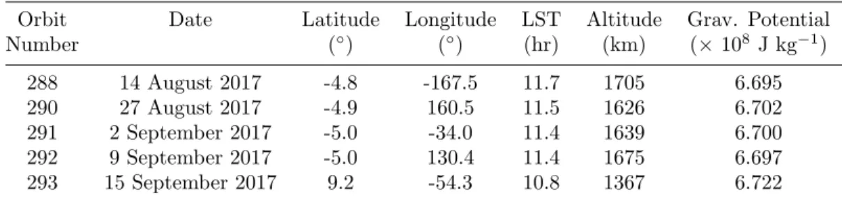
ion-Table 1. Orbital information for the measurements used in this study. These were the last orbits of the Cassini spacecraft and represented the lowest altitude sampling of Saturn’s upper atmosphere. Cassini entered Saturn’s atmosphere during orbit 293.

Orbit Date Latitude Longitude LST Altitude Grav. Potential

Number (◦) (◦) (hr) (km) (× 108 _{J kg}−1₎ 288 14 August 2017 -4.8 -167.5 11.7 1705 6.695 290 27 August 2017 -4.9 160.5 11.5 1626 6.702 291 2 September 2017 -5.0 -34.0 11.4 1639 6.700 292 9 September 2017 -5.0 130.4 11.4 1675 6.697 293 15 September 2017 9.2 -54.3 10.8 1367 6.722

Note. Values in this table correspond to the spacecraft’s closest approach to Saturn. Spacecraft velocity at this time was between 30.1 to 31 km/s for these orbits. LST = local solar time.

ization. Thus, it is likely that a fraction of the signal recorded by the instrument is from fragments of larger particles outside of the instrument’s mass range. However, as reported in Waite et al. (2018), the abundance of larger organics seen in the spectra is at least

an order of magnitude lower than that of CH4 and would not have a very significant

im-pact on the CH4abundance. They also report that the H2 profile derived from INMS

before and after closest approach suggests that effects from the spacecraft’s speed are negligible in close proximity to the planet. Other recent studies also find no significant effects on the measurements from the spacecraft’s high speed (Yelle et al., 2018; Perry et al., 2018; Miller et al., 2020) and our analysis thus far shows no evidence of issues stem-ming from the spacecraft’s speed.

Many factors affect the response of the instrument. These factors have been ex-tensively characterized for Titan’s atmosphere and methods for correction are detailed in Cui et al. (2008), Magee et al. (2009), Cui et al. (2009a), and Cui et al. (2012). We adopt similar methods here and recharacterize the corrections to ensure that they are suitable for Saturn conditions. These include background subtraction and corrections for detector dead-time, calibration sensitivity, ram pressure enhancement, and counter saturation, which are briefly explained below.

Residual gas present in the INMS chamber is responsible for outgassing and en-hancing the signal in certain mass channels. Far from Saturn, this background tends to a constant level which must be properly subtracted in order to remove this enhancement. To determine the mean background signal for each orbit we average data taken well be-fore closest approach to Saturn where signal in mass channel 2 has not yet begun to in-crease, which would indicate the detection of Saturn’s extended atmosphere. The radi-ation background, which is a mass independent enhancement in signal that is due mainly to detection of charged particles from Saturn’s magnetosphere, must also be removed. We determine the radiation background using the signal in mass channels 5 to 8, where no signal is expected and thus the only signal detected here is due to external radiation. The region of the mass spectrum analyzed in this study has a very strong signal in Sat-urn’s atmosphere, thus the background effects are not very significant. However, proper removal of the background signal is critical and is even more crucial when analyzing the signal in higher mass channels where signal is much lower but still present.

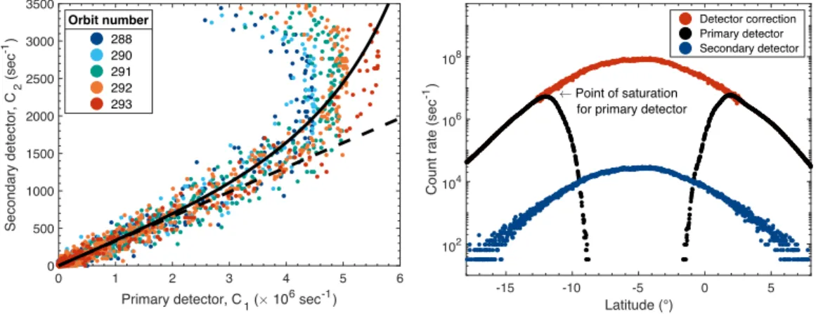
The instrument’s dual detector system includes a high gain primary detector which is known to saturate near closest approach in mass channels relevant to the most abun-dant species in the atmosphere. This leads to signal decay at closest approach as seen in Figure 1. When this occurs, counts from the secondary detector, albeit with a lower signal-to-noise ratio, can be utilized to obtain an accurate determination of the density

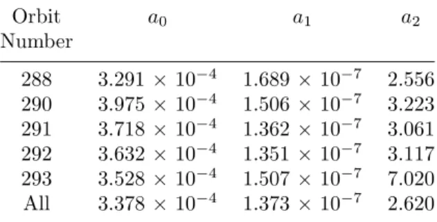
Table 2. Free parameters used in the empirical relationship between the count rates from the primary and secondary detectors for mass channel 2 (H2.)

Orbit a0 a1 a2 Number 288 3.291 × 10−4 1.689 × 10−7 2.556 290 3.975 × 10−4 1.506 × 10−7 3.223 291 3.718 × 10−4 1.362 × 10−7 3.061 292 3.632 × 10−4 1.351 × 10−7 3.117 293 3.528 × 10−4 1.507 × 10−7 7.020 All 3.378 × 10−4 1.373 × 10−7 2.620

profile. In order to take advantage of the primary detector’s much higher signal-to-noise ratio, we use a nonlinear conversion technique between the primary and secondary de-tectors as detailed in Cui et al. (2012). In doing so, we are able to utilize slightly sat-urated count rates from the primary detector, significantly reducing the amount of noise in the density profile. Saturation of the primary detector is a species dependent process. At Titan, detector saturation occurred in mass channels associated with the atmosphere’s

major constituents, N2 and CH4, at m/z 14, 15, 16, 28, and 29 amu. At Saturn, the only

channel that experiences saturation is m/z 2 amu, which tracks H2 in the atmosphere.

This saturation can be seen in Figure 1, where the count rate from the primary detec-tor in mass channel 2 is plotted against the count rate from the secondary detecdetec-tor for all of the final orbits. At lower counts the detectors are linearly correlated but as the count rate of the primary detector increases, the signal begins to decay and the detectors lose their linear correlation. The relationship between the detectors can be described using an empirical equation, as described in Cui et al. (2012):

C2= a0C1exp{tan[(a1C1)a2]}, (1)

where a0, a1, and a2 are free parameters constrained by the data. The free param-eters for each orbit are listed in Table 2. Characterizing this relationship allows us to

use slightly saturated counts from the primary detector up to 4.2 × 106 counts/s. At this

point, the empirical relationship no longer traces the primary detector’s signal decay and the correction is no longer applicable, prompting the use of counts from the secondary counter. However, an instantaneous switch from the primary to secondary detector at

4.2 × 106 counts/s could introduce discontinuities in the derived density profiles, which

in turn would affect the retrieved temperature profile. To remove this effect, we intro-duce continuously varying weighting functions to calculate densities in the transition re-gion as detailed in Cui et al. (2012).

The INMS flight unit (FU) was calibrated with neutral species relevant to Titan’s atmosphere before launch and additional calibration of other species continued after launch using the identical engineering unit (EU). Thus, a calibration database to compare known fragmentation patterns to observed measurements exists. Due to response differences be-tween the FU and EU, calibration of the peak sensitivity of each species must be per-formed in order to utilize EU calibration measurements to understand observations us-ing the FU. Cui et al. (2009a) developed an algorithm to characterize these sensitivity differences based on measurements of species that were calibrated using both units and we utilize these results here since many of these molecules are also relevant to Saturn’s upper atmosphere. Additionally, the ram pressure of the inflowing sample in CSN mode leads to a density enhancement in the instrument that varies as a function of

molecu-0 1 2 3 4 5 6 Primary detector, C₁ ( 106 sec-1) 0 500 1000 1500 2000 2500 3000 3500 Secondary detector, C 2 (sec -1) 288₂₉₀ 291 292 293 Orbit number -15 -10 -5 0 5 Latitude (°) 102 104 106 108

Count rate (sec

-1) Point of saturation for primary detector

Detector correction Primary detector Secondary detector

Figure 1. Left: Count rate in mass channel 2 (H2) from the secondary detector (C2) as a function of count rate in mass channel 2 from the primary detector (C1) for all five orbits an-alyzed here. The dashed line represents the linear correlation between these detectors at lower count rates and is the trend that the signal would follow if the primary detector was not affected by saturation. The solid line represents the nonlinear empirical relationship (equation 1) used to correct for saturation in the primary detector. Doing so increases the signal to noise ratio in our results and allows us to use measurements from the primary detector up to 4.2 × 106 counts/s. Right: Count rate of both detectors in mass channel 2 as a function of latitude for orbit 290. Closest approach to Saturn, where the signal is highest, occurs near -5◦latitude. As the space-craft approaches Saturn, the primary detector (black) saturates which leads to a signal decay, while the lower signal secondary detector (blue) does not. We are able to combine measurements from both detectors and determine a corrected count rate to be used to determine a proper H2 density in Saturn’s atmosphere (red).

lar mass, angle of attack of the instrument, temperature of the ambient gas, and speed of the spacecraft. This ram enhancement factor was previously characterized in Cui et al. (2009a) for Titan flybys, and we use the same approach to correct for the ram enhance-ment factor here. Corrections for contamination from thruster firings of the spacecraft, which occasionally affect the counts in mass channel 2 during Titan flybys, are not done here since thrusters were not used near closest approach for these final orbits.

Additionally, Saturn’s high rotation rate and significantly oblate shape invalidates the common assumption that atmospheric variations are purely radial. Instead, we as-sume here that Saturn’s atmospheric properties vary with gravitational potential, φ, and we use φ as the vertical coordinate in our analysis. This modification includes adopt-ing the updated gravitational potential for Saturn found in Anderson and Schubert (2007). This process is detailed in the supporting information of Yelle et al. (2018).

Although the instrument records data before and after closest approach to the planet, our analysis utilizes solely inbound data. INMS has a well-documented behavior where certain species entering the instrument adsorb to the chamber’s walls. This adsorption can lead to wall chemistry within the instrument and/or desorption at a later time (see e.g., Cui et al. (2008); Vuitton et al. (2008); Cui et al. (2009a)). This effect is observed near closest approach to the planet, when the number density of molecules is highest, and predominantly affects outbound measurements which leads to an artificial outbound density enhancement for certain species. For this reason, we do not utilize these mea-surements here and focus on direct inbound meamea-surements.

While wall adsorption leads to difficulties in properly interpreting the outbound measurements for some mass channels, this effect is actually valuable in determining what species might be present in the measurements. Only certain species are affected by wall

adsorption and subsequent chemistry within the instrument. Inert species and CH4 are

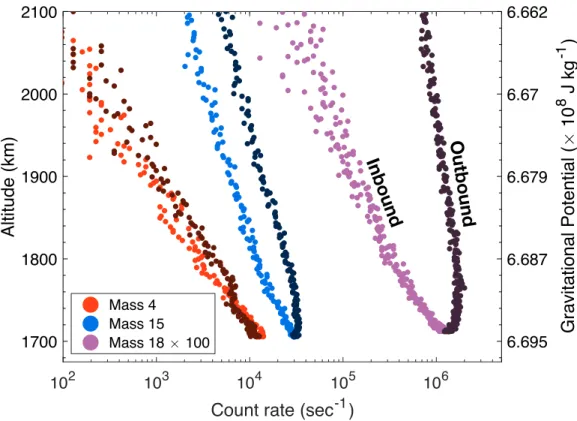
known not to contribute to wall adsorption (see e.g., Cui et al. (2008, 2009a)), whereas other species, such as H2O and NH3, exhibit significant effects due to wall adsorption. Using this knowledge, it can be deduced whether certain species are present in the mea-surements based solely on the inbound/outbound asymmetry of relevant mass channels. An example of this is seen in Figure 2. Mass channel 4, which tracks He (an inert species), exhibits a symmetric profile before and after closest approach. On the other hand, mass

channel 18, which tracks H2O, exhibits a significant asymmetric distribution before and

after closest approach indicative of wall effects for this species. Mass channel 15 is

pri-marily a combination of signal from fragments associated with CH4 and/or NH3. The

asymmetric distribution implies that the signal measured in this mass channel must have

some contribution from NH3 since the signal from a lack of NH3would have had no

asym-metry at closest approach. In this figure, the left axis of altitude is the height above Sat-urn’s 1-bar pressure level that corresponds to the gravitational potential values seen on the right axis. The profile of inbound measurements for mass channels 15 and 18 sug-gests that measurements in these channels directly before closest approach (below φ of

approximately 6.69 × 108 J kg−1 (1750 km) could also be slightly affected by a density

enhancement for orbits 288 to 292. Proper correction for this enhancement would require extensive knowledge of how each species interacts within the chamber and subsequent modeling to correct for this asymmetry and is beyond the scope of this paper.

3.2 Mass spectral deconvolution

Species identification and density determination from INMS measurements is com-plicated by the fact that multiple species contribute to the signal of individual mass chan-nels, creating a complex combination of mass peaks associated with a mix of the frag-mentation patterns of the species within the sample. An accurate density determination of species within the atmosphere must begin by first determining the relative contribu-tion of each species to each mass channel. This is done by combining the peak

intensi-10

10

10

10

10

Count rate (sec

)

1700

1800

1900

2000

2100

Altitude (km)

6.695

6.687

6.679

6.67

6.662

Gravitational Potential (

10

J kg

)

Inbound

Outbound

Figure 2. Count rate of mass channels 4, 15, and 18 as a function of altitude and gravita-tional potential from orbit 290. The lighter shade for each mass channel represents the inbound profile and the darker shade represents the outbound profile. The inbound and outbound profiles of mass channel 4 (He) are nearly identical since this species does not adsorb to the instrument’s chamber walls or participate in wall chemistry. Mass channel 18 (H2O) is known to be affected by wall adsorption and chemistry in the instrument, which is the reason for the significant in-bound/outbound asymmetry. Mass channel 15 is a combination of signal from CH4 and NH3. Since CH4 is not affected by wall adsorption in the instrument, this asymmetry indicates that NH3must be contributing to the signal.

ties of the fragmentation patterns of each species from calibration data weighted by a relative contribution from each species that results in the best fit to the measured mass spectrum. Thus, one must solve a system of linear equations:

Ii= n X

j=1

Fi,jNj (2)

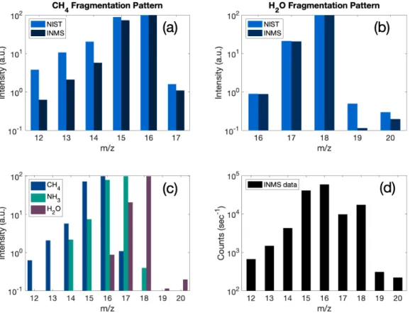
The relative intensities of the fragmentation peaks produced by a certain species are highly dependent on the instrument used, thus it’s crucial to have an accurate instrumental frag-mentation pattern database to compare to observations returned by the spacecraft. As stated above, we focus here on the region of the mass spectrum from 12 to 20 amu and

the primary species contributing to this region: CH4, H2O, and NH3. An example of the

signal measured by INMS in this region is shown in Figure 3d for orbit 290. Figure 3c compares the overlapping fragmentation patterns of these three species from calibration data. Although INMS was calibrated for many species relevant to both Titan and

Sat-urn, unfortunately the instrument was never calibrated for NH3. As a consequence,

cal-ibration data from the National Institute of Standards and Technology (NIST) mass

spec-tral library must be utilized for NH3. Figures 3a and b compare the INMS calibration

data of CH4 and H2O to data from NIST. Although NIST calibrations provide an

ad-equate estimate on what to expect during the flight instrument’s performance, there are significant deviations in fragmentation peak intensity in certain mass channels for both species. Furthermore, the instrument’s calibration on Earth was performed in an envi-ronment very different from that of Saturn, which could lead to discrepancies between the fragmentation patterns found in the calibration database and the actual measure-ments returned from the instrument. Deviations stemming from the aging of the instru-ment, which was launched in 1997, could also affect the instrument’s performance over time and lead to further discrepancies between calibration values and returned measure-ments. Although a calibration database is of utmost importance, an accurate and com-plete database of fragmentation patterns relevant to this study does not exist.

In order to overcome the challenges brought about by the calibration data from INMS, our mass spectral deconvolution algorithm employs a Monte-Carlo based approach to handle the uncertainty in fragmentation peak intensities of each species (Gautier et al., 2019). The Monte-Carlo randomization is applied only to the intensity (y-axis) of each fragmentation peak for each species in the database, not to the m/z ratio (x-axis) of the fragmentation peaks. We allow for ±15% variation in individual peak intensities from the original database, which is a combination of INMS calibration data and NIST val-ues when INMS data is unavailable. This process is done 500,000 times, thus creating 500,000 individual fragmentation databases that are then used to decompose the mea-sured mass spectrum. The output of the deconvolution includes the relative abundances of each species in the database based on the randomized fragmentation pattern database that was input into the model. We keep the best-fitting 2% (best-fitting 10,000 mass spec-tral fits) of these simulations for analysis based on the outputs with the minimal resid-uals to the data. This allows us in the end to retrieve a statistical solution to our issue, providing the most probable concentration for a given species as well as a probability

density function (PDF) in order to quantify the variation in a species’ concentration through-out the best-fitting simulations saved for analysis. Although we allow the peak

inten-sities to vary by 15%, the main peaks for the best-fitting simulations saved for analy-sis vary by only a few percent and the less significant peaks typically vary no more than ∼10%.

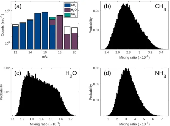
In solving for the relative concentration of each species, we are able to determine the mixing ratio for these species from our model. An example of a mass spectral fit along with PDFs is shown in Fig. 4 for orbit 290 with an averaged mass spectrum from a grav-itational potential height of 6.69 to 6.66 × 108 J kg−1. The black outline bars in Fig-ure 4 show the measFig-ured mass spectrum and the colored bars represent the modeled con-tribution of each molecule to the mass channel. For this study, we use H2, He, CH4, H2O,

Figure 3. (a and b) Comparison of INMS and NIST calibration data for CH4 (a) and H2O (b). The differences in fragmentation peak intensities, along with a lack of INMS calibration data for some species, complicate analysis of the spectra returned by INMS. (c) Overlapping fragmen-tation patterns of CH4, H2O, and NH3 which all contribute to the INMS signal in the region m/z = 12 - 20 amu. CH4 and H2O data are from INMS calibration measurements. NH3 data are from the NIST spectral library. (d) Signal from INMS from orbit 290 extracted between φ of 6.69 and 6.66 × 108 _{J kg}−1

and NH3 to fit the mass spectrum up to 20 amu. There is no signal detected from 5 to

11 amu. The signal below 5 amu is predominantly from H2 and He, and above 11 amu

is a combination of CH4, H2O, and NH3. A detailed analysis for H2and He was

pub-lished previously in Yelle et al. (2018). These species will be discussed here only for com-parison and are included in our modeling in order to retrieve accurate mixing ratio in-formation since these are the two major constituents of Saturn’s atmosphere. We assume

that the region from 12 to 20 amu is contributed only by CH4, H2O, and NH3. In

re-ality, it is likely that fragments of other molecules with higher masses also contribute to these mass channels. However, higher mass species will not dissociate into fragments that

contribute significantly to the predominant peaks associated with CH4, H2O, and NH3

(16, 17, and 18 amu), so the small contributions from the fragments of higher mass species are not included in this study. These fragments will mostly contribute to mass channels 12 and 14 amu (corresponding to signal from ionized carbon and nitrogen, respectively), which are consistently underfit by our model. As a consequence, the results presented

here should be considered upper limits for the mixing ratios of CH4, H2O, and NH3.

Fu-ture work will address the entirety of the mass spectrum (up to 99 amu), which could result in a slight revision to the mixing ratio values presented here. In any case, the mod-eled spectra provide reasonable fits to the data, with the major peaks from 15 to 18 amu being reproduced by the model very well. Mass channels 19 and 20, whose signal has

con-tributions from isotopes of H2O, are underfit by our current modeling efforts. The

sig-nal at 19 amu is significantly higher than expected and could be a consequence of con-tamination from filament desorption (see e.g., Perry et al. (2010, 2015)), however this source of background contamination is poorly quantified. Mass channel 20 could have contributions from other molecules at higher masses, including argon which contributes

to the signal as Ar2+_{. Nonetheless, accurate measurements of isotopes for these species}

are beyond the scope of this paper and will be addressed in upcoming work. 3.3 Density determination

After correcting the raw INMS counts as described above, we are able to utilize the mass spectral deconvolution algorithm to derive number density profiles for the species. In order to do so, the count rates for each mass channel are divided into bins with a width

of φ = 0.01 J kg−1 and the deconvolution is performed for each separate gravitational

potential bin. The average output of the best-fitting 2% of simulations is then used to determine the relative contribution of each species to its dominant mass channel. This

is done using mass channels 16, 17, and 18 amu, which are the molecular peaks of CH4,

H2O, and NH3, respectively, and have very high signal. CH4 and H2O both have peaks

which are relatively free of significant contamination by other species: 12 and 13 amu

for CH4, and 18 to 20 amu for H2O. This, along with comparison to the peak

intensi-ties within the region where there is contribution from other species, provides convinc-ing evidence that these species are in fact present in the measured mass spectrum. The

NH3 contribution, on the other hand, must be constrained by mass channel 17, which

is the species’ parent peak but has significant contribution from both CH4and H2O. Thus,

NH3 detection and quantification relies more heavily on our modeling efforts than that

of CH4 and H2O. However, as stated previously, there is evidence that NH3is present

within the spectrum due to the asymmetry of the measurements around closest approach as shown in Figure 2.

We utilize counts from the instrument as long as the signal-to-noise ratio is suffi-cient for analysis. For He, H2O, and NH3, the loss of signal occurs at a higher φ (lower

altitude) than CH4 and H2 due to the lower abundance of these three species in the

re-gion. Thus, we obtain density profiles for H2and CH4 that extend to a lower φ (higher

altitude) from closest approach than the other species. After running the Monte Carlo algorithm described above, we determine the density profiles by weighting the corrected count rate from the species’ main mass channel with the relative contribution of that species returned by the model for each φ bin. Results using this method are shown in Fig. 5.

12 14 16 18 20 m/z 100 105 Counts (sec -1)

(a)

(b)

CH

(c)

H

O

(d)

NH

Figure 4. (a) Example of mass spectrum deconvolution result using our Monte-Carlo ap-proach for orbit 290. Black outline bars represent the measured INMS spectrum. Colored seg-ments represent the contribution of each species as calculated by the model. Contributions shown here are the average contribution of the best-fitting 2% of 500,000 simulations. (b–d) Probabil-ity densities of the mixing ratio of each species in the sample as retrieved by the model for the best-fitting 2% of simulations.

Running independent simulations in each φ bin provides us with reasonable results for each species. The average output of each φ bin from the best-fitting 2% of simulations is then combined to create a density profile, which produces smooth and consistent pro-files for each species. This consistency demonstrates the power of our new method in help-ing to determine the contribution of each species when the available calibration data for an instrument is insufficient. Errors associated with these density profiles are a combi-nation of 1σ uncertainties due to counting statistics from the data and 1σ standard

de-viation from the modeling results. H2 and He have a higher signal-to-noise ratio in their

dominant mass channels and are better constrained by the model, leading to small er-rors associated with these species. They are also well constrained by the model since there is no interference from other species in their relevant mass channels. Measurements for

H2O and NH3have a lower signal and these species have a greater spread in the

mod-eling results, leading to slightly larger error bars for these species. The retrieved errors

associated with the density profiles in Fig. 5 for all molecules but H2 range from a few

percent near closest approach, where signal is highest, and increase to approximately 50%

for the uppermost measurements where signal is much lower. Errors in the H2density

profile are no more than 10% for the region of the atmosphere analyzed here.

4 Results and Discussion

4.1 Density profiles and mixing ratios

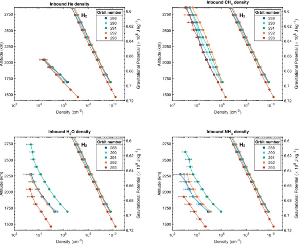
Density profiles of H2, He, CH4, H2O, and NH3 from Cassini’s last orbits are shown in Figure 5. Although these results agree with and are an extension of the work presented in Yelle et al. (2018), we obtain the density profiles of H2, He, and CH4 using slightly different methods. In Yelle et al. (2018), we obtain density profiles of these species by using the corrected measurements in the dominant mass channels for each species (m/z 2, 4, and 16 amu, respectively) without fitting the mass spectrum. This method is rea-sonable since there is very little interference from other species in these three mass

chan-nels. In order to expand our analysis to H2O and NH3, we determine density profiles by

binning the data and employing the mass spectral deconvolution as described above. Our

new method does not modify the results of H2 and He since there is no overlapping

sig-nal in their dominant mass channels. The results of CH4are changed by about 2% on

average, which is well within the errors associated with the measurements.

We obtain density profiles for CH4 from closest approach for each orbit up to φ of

approximately 6.59 × 108 J kg−1 (2850 km) and for He from closest approach up to φ

of approximately 6.67 × 108 J kg−1 (2050 km). H2O and NH3show greater variability

in their density profiles from orbit to orbit, leading to differences in signal and conse-quently differences in the extent of their retrieved density profiles. The profiles presented here provide further evidence from INMS for an external source providing Saturn’s up-per atmosphere with a variety of unexpected species, as previously reported in Yelle et al. (2018); Waite et al. (2018); Perry et al. (2018); Miller et al. (2020). The density of

species as heavy as CH4, H2O, and NH3should decrease rapidly above Saturn’s homopause

as a consequence of diffusive separation. However, the scale heights of these species and their presence in this region of the atmosphere are inconsistent with these species be-ing native to Saturn’s interior and emergbe-ing via upward diffusion. He, on the other hand, decreases rapidly above the homopause and follows the expected scale height and

den-sity profile of a molecule of its mass in a H2-dominated atmosphere.

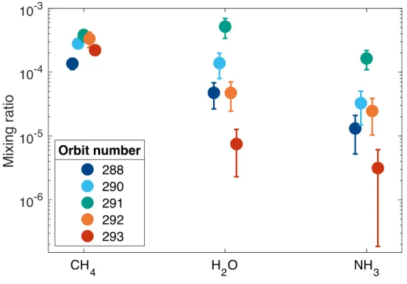
Figure 6 shows the average mixing ratio for each species for each orbit. In order to compare the orbits, we determine these mixing ratios using an averaged mass spec-trum that incorporates the region of the atmosphere where all five orbits have reliable data. This corresponds to the region of the atmosphere of approximately 6.69 to 6.66

× 108 _{J kg}−1 _{(1700 to 2050 km). One notable observation is the variability of these}

102 ₁₀4 ₁₀6 ₁₀8 ₁₀10 Density (cm-3₎ 2750 2500 2250 2000 1750 1500 Altitude (km) 6.6 6.62 6.64 6.66 6.68 6.7 6.72 Gravitational Potential ( 10 8 J kg -1) Inbound He density 288 290 291 292 293 Orbit number 102 ₁₀4 ₁₀6 ₁₀8 ₁₀10 Density (cm-3₎ 2750 2500 2250 2000 1750 1500 Altitude (km) 6.6 6.62 6.64 6.66 6.68 6.7 6.72 Gravitational Potential ( 10 8 J kg -1) Inbound CH₄ density 288 290 291 292 293 Orbit number 102 ₁₀4 ₁₀6 ₁₀8 ₁₀10 Density (cm-3₎ 2750 2500 2250 2000 1750 1500 Altitude (km) 6.6 6.62 6.64 6.66 6.68 6.7 6.72 Gravitational Potential ( 10 8 J kg -1) Inbound H₂O density 288 290 291 292 293 Orbit number 102 ₁₀4 ₁₀6 ₁₀8 ₁₀10 Density (cm-3₎ 2750 2500 2250 2000 1750 1500 Altitude (km) 6.6 6.62 6.64 6.66 6.68 6.7 6.72 Gravitational Potential ( 10 8 J kg -1) Inbound NH₃ density 288 290 291 292 293 Orbit number H2 H2 H2 H2

Figure 5. Inbound density profiles of He, CH4, H2O, and NH3 versus altitude and gravita-tional potential for all five orbits analyzed. The density profiles of H2 are also included in each figure for comparison. Density profiles are constructed by averaging INMS measurements in gravitational potential bins of 0.01 J kg−1, then running a mass spectral deconvolution for each individual bin. Error bars are a combination of 1σ uncertainties from counting statistics and 1σ uncertainties from the mass spectral deconvolution.

entry). All orbits aside from orbit 293 measured Saturn’s atmosphere at similar

condi-tions with closest approach to the planet around 5◦ _{S (see Table 1). Orbit 293, however,}

entered Saturn’s atmosphere around 9◦N before crossing the equatorial ring plane. The

difference in the region sampled for orbit 293 could be the explanation for depletion in

H2O and NH3during atmospheric entry.

The mixing ratio of He shows very little variation and is around 3.0 ±0.2 × 10−4

for this region of the atmosphere. CH4 shows more variability than He, but measurements

are roughly consistent among orbits, ranging from 1.4 to 3.8 × 108_{. The large}

variabil-ity of H2O and NH3 among orbits, as well as the prevalence of CH4 as a dominant

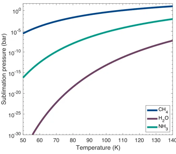
ex-ternal species, are surprising and unexpected, but potential explanations for these re-sults do exist. First, as noted in Yelle et al. (2018), the prevalence of CH4 over H2O and

NH3 could be tied to the volatility of these species. Their sublimation pressures, shown

in Figure 7, vary by orders of magnitude at temperatures relevant to Saturn’s inner rings of ∼80 to 115 K (Filacchione et al., 2014; Tiscareno et al., 2019). Saturn’s rings are con-stantly exposed to magnetospheric plasma, cosmic ray impacts, micrometeorite bombard-ment, and other high energy phenomena, resulting in the ejection of surface ring mate-rial which liberates gas molecules from the rings. If these species are present in the rings and are liberated from ice particles in this way, then it is more likely for emitted H2O

and NH3 molecules to recondense back onto ring particles while CH4 is preferentially lost

into Saturn’s atmosphere.

It is also possible that H2O and NH3 are entering Saturn’s atmosphere from the

rings in a charged form (i.e., H3O+ and NH4+), which would elude detection by INMS.

H2O and NH3have much higher proton affinities (691.0 and 853.6 kJ mol−1, respectively)

than CH4(543.5 kJ mol−1) (Hunter & Lias, 1998), making them more susceptible to

pro-ton transfer. If H2O and NH3 are more easily protonated after liberation from ring

par-ticles, they would not be detected by INMS since the ion mode of the instrument was

limited to masses below 8 amu during these orbits due to the speed of the spacecraft (Cravens et al., 2018; Moore et al., 2018). It is also possible that these charged molecules are trans-ported away from the equatorial region via magnetic field lines and deposited into Sat-urn’s atmosphere at higher latitudes that were not observed by INMS. Indeed, O’Donoghue et al. (2017) recently reported evidence that charged water was entering Saturn’s mid-latitude region from the rings via magnetic field lines. An improved understanding of these potential transport processes will require continued monitoring from ground and space based observations and additional in situ measurements from future missions.

4.2 Flux and mass deposition rate calculations

To quantify the influx of material from the rings, we use a 1-D model to understand the exospheric temperature and external flux in the upper atmosphere. This model is described extensively in the supporting information of Yelle et al. (2018), who use the

model to provide a detailed analysis of the CH4influx into Saturn’s atmosphere. We

fol-low the same method here with the addition of H2O and NH3. Briefly, we assume

hy-drostatic equilibrium and solve the standard diffusion equation with φ as the vertical co-ordinate. The mixing ratio of a species is given by

Xi(φ) = Xi(φ◦) exp Z φ φ◦ dφ0 Di Di+ K mi− ma RT − Z φ φ◦ dφ0 Fi gNa(Di+ K) exp( Z φ φ◦ dφ00 Di Di+ K mi− ma RT ) (3)

where Xi is the mixing ratio of the minor constituent, Di is the molecular diffusion

co-efficient, K is the eddy diffusion coco-efficient, mi is the molecular mass of the minor

con-stituent, ma is the average molecular mass of the atmosphere, R is the gas constant for

H2, T is the temperature, g is the magnitude of the gravitational acceleration, Na is the density of H2, and Fi is the flux of the minor constituent. The first term of this equa-tion represents molecular diffusion within the atmosphere and the second term describes the vertical distribution of a molecule with a non-zero external flux into the atmosphere.

CH

H

O

NH

10

10

10

10

Mixing ratio

₂₈₈

290

291

292

293

Orbit number

Figure 6. Averaged mixing ratios of CH4, H2O, and NH3. We use measurements taken be-tween φ of 6.69 and 6.66 × 108 _{J kg}−1

(1700 to 2050 km), where reliable data for all orbits exist, to create the integrated spectra used to determine mixing ratios. Variability among orbits for these volatile species is evident, especially for orbit 293 (atmospheric entry) which measured a different region of Saturn at closest approach and shows a large depletion in H2O and NH3. Error bars are a combination of 1σ uncertainties from counting statistics and 1σ uncertainties from the mass spectral deconvolution.

50

60

70

80

90

100

110

120

130

140

Temperature (K)

10

10

10

10

10

10

10

Sublimation pressure (bar)

CH

H

O

NH

Figure 7. Sublimation pressure curves for CH4, H2O, and NH3 (Fray & Schmitt, 2009) at temperatures relevant to Saturn’s rings.

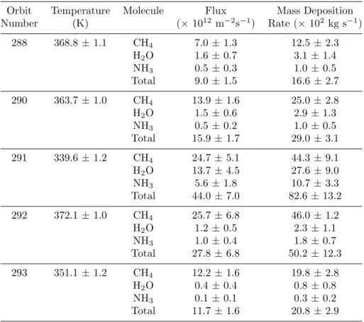
Table 3. Temperature, flux, and mass deposition rate results.

Orbit Temperature Molecule Flux Mass Deposition

Number (K) (× 1012 _m−2_s−1_{) Rate (× 10}2 _{kg s}−1₎ 288 368.8 ± 1.1 CH4 7.0 ± 1.3 12.5 ± 2.3 H2O 1.6 ± 0.7 3.1 ± 1.4 NH3 0.5 ± 0.3 1.0 ± 0.5 Total 9.0 ± 1.5 16.6 ± 2.7 290 363.7 ± 1.0 CH4 13.9 ± 1.6 25.0 ± 2.8 H2O 1.5 ± 0.6 2.9 ± 1.3 NH3 0.5 ± 0.2 1.0 ± 0.5 Total 15.9 ± 1.7 29.0 ± 3.1 291 339.6 ± 1.2 CH4 24.7 ± 5.1 44.3 ± 9.1 H2O 13.7 ± 4.5 27.6 ± 9.0 NH3 5.6 ± 1.8 10.7 ± 3.3 Total 44.0 ± 7.0 82.6 ± 13.2 292 372.1 ± 1.0 CH4 25.7 ± 6.8 46.0 ± 1.2 H2O 1.2 ± 0.5 2.3 ± 1.1 NH3 1.0 ± 0.4 1.8 ± 0.7 Total 27.8 ± 6.8 50.2 ± 12.3 293 351.1 ± 1.2 CH4 12.2 ± 1.6 19.8 ± 2.8 H2O 0.4 ± 0.4 0.8 ± 0.8 NH3 0.1 ± 0.1 0.3 ± 0.2 Total 11.7 ± 1.6 20.8 ± 2.9

We determine the temperature using the H2 density profile for each orbit. For the

plunge, which probes deeper into the atmosphere, we determine the temperature pro-file using a Bates propro-file for a thermosphere (Bates, 1951). The other orbits probe higher in the atmosphere and we determine the temperature by fitting an isothermal model to

the H2density profiles. The temperature results are found in Table 3 and were originally

published in Yelle et al. (2018), where further discussion and interpretation is presented. We also adopt the eddy diffusion profile from Yelle et al. (2018), which has a constant

value in the uppermost region of the atmosphere of K∞ = 1.4 × 104 m2s−1, although

a wide variety of K profiles can be used to fit the data. The molecular diffusion

coeffi-cients for He and CH4in H2 are taken from Mason and Marrero (1970). We calculate

the molecular diffusion coefficients for H2O and NH3 in H2with the theoretical approach

outlined in Hirschfelder et al. (1954) based on the Lennard-Jones potential. Molecular diffusion coefficients for these species at φ of 6.69 × 108_{J kg}−1 _{are 1.3 × 10}6 _m2_s−1 _for He, 6.2 × 105 _m2_s−1 _{for CH}

4, 8.0× 105m2s−1 for H2O, and 8.4 × 105m2s−1 for NH3. Helium is native to the planet and exhibits a mixing ratio decreasing with altitude in accordance with a species following diffusive separation in a well-mixed atmosphere.

Thus, our model needs no external flux (Fi = 0) to properly fit the He measurements.

On the other hand, H2O, CH4, and NH3 all exhibit roughly constant mixing ratios in

the upper atmosphere, which is expected for a minor constituent entering the atmosphere externally (Connerney & Waite, 1984). To determine the external flux we utilize inbound

measurements taken before the slight density enhancement observed for H2O and NH3,

which excludes measurements taken below φ of 6.69 × 108 J kg−1 (1750 km) for orbits

288 to 292. Measurements can be fit using a constant external flux and results for all orbits are found in Table 3.

The variability in the influx of external material measured among orbits, especially

for H2O and NH3, leads to large fluctuations in the observed amount of material deposited

into the atmosphere. We quantify the mass deposition rate (MDR) for each species into the atmosphere using the equation

M DR = Fimi× 2πrSaturn2 θ, (4)

where Fi is the flux of molecule i, mi is the molecular mass of molecule i, and the sec-ond term represents the surface area of Saturn that is affected by the deposition of

ex-ternal material. We use a latitudinal width (θ) for the influx region of 16◦. This width

corresponds to the location at which we observe a decrease in signal of the minor

con-stituents, which occurs at approximately ±8◦ from the ring plane. It is possible that the

affected region of Saturn is larger than this, however a larger width cannot be deduced from our measurements due to the loss of signal.

Mass deposition rates for all three species are found in Table 3. Although

previ-ous studies indicate that the rings are composed overwhelmingly of H2O ice (see recent

review by Cuzzi, Filacchione, and Marouf (2018) and references therein), we find that

CH4represents the largest fraction of the total MDR in our results. Previous remote

ob-servations do indicate the presence of a non water ice component to the rings, however no study has definitively determined the composition of this material. In fact, discreet

searches for spectral features of CH4 and NH3 in ring observations found no significant

amounts of either species (Nicholson et al., 2008). Recent in situ Grand Finale obser-vations using Cassini’s Cosmic Dust Analyzer (CDA) observed a much higher silicate frac-tion in the D ring than previously inferred from optical and microwave measurements (Hsu et al., 2018). It remains unclear why in situ measurements from INMS and CDA observe a much more significant fraction of non water ice material in the rings. Remote observations suggest that the non water material is intimately mixed within the water ice grains (Filacchione et al., 2014; Cuzzi, French, et al., 2018). If these minor compo-nents exist in the rings as inclusions within water ice grains or as clathrates, it is pos-sible that the resolution of existing remote observations cannot distinguish the signal from pure water ice. If water ice is deposited back onto ring particles as suspected it is also possible that the water ice is shielding the spectroscopic signature of the minor constituents within the rings, which could be part of the reason that non water ice components have evaded detection via remote observations.

H2O and NH3exhibit greater variations in deposition rate than CH4 from orbit

to orbit, with a tenfold increase observed during orbit 291. In total, the mass deposition

rate into Saturn for these three species spans from 1.7 to 8.3 × 103 kg/s. This is a

sub-stantial amount of incoming material and these results represent a lower limit on the amount entering Saturn from the rings since we are focusing here only on a limited set of the full mass range of the instrument. INMS detected many other species with higher mass also entering Saturn’s atmosphere (Waite et al., 2018). Using different methods, Waite et al.

(2018) and Perry et al. (2018) reported >104 _{kg/s of material entering the atmosphere}

based on INMS observations. This higher mass material is beyond the scope of this pa-per and will be discussed in upcoming publications.

Recent Grand Finale results suggest that the mass of Saturn’s rings is actually lower

than most previous results, approximately 1.54 ± 0.49 × 1019 _{kg (Iess et al., 2019). If}

we use very straightforward assumptions that the rings are able to spread over time (via viscous spreading, satellite interactions, and micrometeoritic bombardment) and contin-uously feed the influx of material into the atmosphere, that our influx values are con-stant over time, and that there are no other sources replenishing the rings, then our mass deposition results suggest that the entire ring system could be depleted in approximately 120 million years. More realistically, viscous spreading throughout the rings is not ef-fective enough to deplete the entirety of the ring system (Salmon et al., 2010). The bulk of this infalling material is coming from Saturn’s diffuse innermost D ring, which could

result in an extremely short lifetime for the D ring and no notable effects for the more massive rings that are located further from the planet. The D ring is most likely sustained over time by material from the neighboring C ring, so it is possible that this influx is also affecting the C ring. Furthermore, observations of the D ring since the Voyager era in-dicate that it is rather dynamic and recent disturbances within the ring (Hedman et al., 2007, 2014) suggest that this large influx could be a recent and temporary development. If this is the case, the large influx of material observed in Cassini’s last orbits might be a transient episode that is not indicative of typical influx values.

5 Conclusions

Cassini’s Grand Finale orbits performed the first ever in situ observations of Sat-urn’s upper atmosphere. The surprisingly complex measurements returned by INMS pro-vide us with the unique opportunity to measure the composition of the rings and under-stand the impact of ring rain on Saturn’s equatorial atmosphere. In this study, we present further evidence of ring material inflowing into Saturn’s upper atmosphere from Cassini’s last few orbits, building on previous INMS results first reported in Yelle et al. (2018). The region of the INMS mass range presented here (m/z = 12 - 20 amu) indicates that

CH4, H2O, and NH3are entering Saturn’s equatorial region through dynamic ring-atmosphere

interactions. We have not analyzed here the entirety of the mass range (up to 99 amu), which includes evidence for a large amount of higher mass organics also present in Sat-urn’s upper atmosphere, and will be discussed in future work.

Identification and quantification of these species in the returned mass spectra are made difficult by their overlapping signals in INMS measurements. This is further com-plicated by the fact that INMS calibration data do not exist for all species of interest and measurements from the standard NIST mass spectral library are not an identical substitute for INMS calibration values. To overcome this, we adopt a new approach to mass spectral deconvolution that uses a Monte-Carlo randomization of the peak inten-sity of each fragment for each species (Gautier et al., 2019). This method allows us to generate thousands of simulated databases to model the INMS measurements and pro-vides a probability density for the mixing ratio of each species in the database. Retrieved

mixing ratios confirm the presence of a large abundance of CH4 as previously reported

in Yelle et al. (2018) and Waite et al. (2018), and highlight the variability of CH4, H2O, and NH3. This variability could be connected to the volatility of these species or their

differing proton affinities, which could allow for H2O and NH3to more readily enter

Sat-urn’s atmosphere from the rings in a charged form at different latitudes.

Retrieved density profiles of these species, along with Saturn’s main atmospheric

constituents H2and He, show that while He is in diffusive equilibrium above the homopause

as expected, CH4, H2O, and NH3are not. Their presence in this region of the atmosphere

and their nearly constant mixing ratio is consistent with an external source, which must

be Saturn’s rings. The measured influx for these orbits ranges from 9 to 44 × 1012_m−2_s−1_,

which translates to 1.7 to 8.3 × 103 _{kg s}−1 _{being deposited into Saturn’s atmosphere.}

These results represent a lower limit on the influx from INMS observations and are thus far consistent with previous INMS measurements (Waite et al., 2018; Perry et al., 2018), and further expand on observations of ring-atmosphere interactions (e.g., Connerney and Waite (1984); O’Donoghue et al. (2017); Hsu et al. (2018); Mitchell et al. (2018)).

Acknowledgments

This research was supported by Grant 80NSSC19K0903 originally selected as part of the Cassini Data Analysis Program, and now supported by NASA’s Planetary Science Di-vision Internal Scientist Funding Program through the Fundamental Laboratory Research (FLaRe) work package, and 16-CDAP16 2-0087. The original INMS data analyzed here

https://pds-ppi.igpp.ucla.edu/search/view/?f=yes&id=pds://PPI/CO-S-INMS-3-L1A-U-V1.0/DATA/SATURN/2017. Data generated as a result of this anal-ysis can be found in the Johns Hopkins University Data Archive with the following DOI https://doi.org/10.7281/T1/QGOMA0.

References

Anderson, J. D., & Schubert, G. (2007). Saturn’s gravitational field, internal

rota-tion, and interior structure. Science, 317 (5843), 1384–1387.

Bates, D. R. (1951). The temperature of the upper atmosphere. Proceedings of the Physical Society. Section B , 64 (9), 805.

Connerney, J. E. P., & Waite, J. H. (1984). New model of Saturn’s ionosphere with an influx of water from the rings. Nature, 312 (5990), 136.

Cravens, T. E., Moore, L., Waite, J. H., Perryman, R., Perry, M., Wahlund, J. E.,

. . . Kurth, W. S. (2018). The ion composition of Saturn’s equatorial

iono-sphere as observed by Cassini. Geophysical Research Letters.

Cui, J., Galand, M., Yelle, R. V., Vuitton, V., Wahlund, J. E., Lavvas, P. P., . . .

Waite, J. H. (2009b). Diurnal variations of Titan’s ionosphere. Journal of

Geophysical Research: Space Physics, 114 (A6).

Cui, J., Yelle, R. V., Strobel, D. F., M¨uller-Wodarg, I. C. F., Snowden, D. S.,

Kosk-inen, T. T., & Galand, M. (2012). The CH4 structure in Titan’s upper

atmo-sphere revisited. Journal of Geophysical Research: Planets, 117 (E11).

Cui, J., Yelle, R. V., & Volk, K. (2008). Distribution and escape of molecular

hydro-gen in Titan’s thermosphere and exosphere. Journal of Geophysical Research:

Planets, 113 (E10).

Cui, J., Yelle, R. V., Vuitton, V., Waite, J. H., Kasprzak, W. T., Gell, D. A., . . . others (2009a). Analysis of Titan’s neutral upper atmosphere from Cassini Ion Neutral Mass Spectrometer measurements. Icarus, 200 (2), 581–615.

Cuzzi, J. N., Filacchione, G., & Marouf, E. A. (2018). The Rings of Saturn. In

M. S. Tiscareno & C. D. Murray (Eds.), Planetary ring systems:

Proper-ties, structure, and evolution (p. 51-92). Cambridge University Press. doi:

10.1017/9781316286791.003

Cuzzi, J. N., French, R. G., Hendrix, A. R., Olson, D. M., Roush, T., & Vahidinia, S. (2018). HST-STIS spectra and the redness of Saturn’s rings. Icarus, 309 , 363–388.

Filacchione, G., Ciarniello, M., Capaccioni, F., Clark, R. N., Nicholson, P. D.,

Hed-man, M. M., . . . others (2014). Cassini–VIMS observations of Saturn’s main

rings: I. Spectral properties and temperature radial profiles variability with phase angle and elevation. Icarus, 241 , 45–65.

Fray, N., & Schmitt, B. (2009). Sublimation of ices of astrophysical interest: A bibli-ographic review. Planetary and Space Science, 57 (14-15), 2053–2080.

Gautier, T., Serigano, J., Bourgalais, J., H¨orst, S. M., & Trainer, M. G. (2019).

Decomposition of electron ionization mass apectra for space application using a Monte-Carlo approach. Rapid Communications in Mass Spectrometry . Hedman, M. M., Burns, J. A., Showalter, M. R., Porco, C. C., Nicholson, P. D.,

Bosh, A. S., . . . others (2007). Saturn’s dynamic D ring. Icarus, 188 (1),

89–107.

Hedman, M. M., Burt, J. A., Burns, J. A., & Showalter, M. R. (2014). Non-circular features in Saturn’s D ring: D68. Icarus, 233 , 147–162.

Hirschfelder, J. O., Curtiss, C. F., Bird, R. B., & Mayer, M. G. (1954). Molecular

theory of gases and liquids (Vol. 26). Wiley New York.

Hsu, H.-W., Schmidt, J., Kempf, S., Postberg, F., Moragas-Klostermeyer, G., Seiß,

M., . . . others (2018). In situ collection of dust grains falling from Saturn’s

rings into its atmosphere. Science, 362 (6410), eaat3185.

Hunter, E. P. L., & Lias, S. G. (1998). Evaluated gas phase basicities and proton

Data, 27 (3), 413–656.

Iess, L., Militzer, B., Kaspi, Y., Nicholson, P., Durante, D., Racioppa, P., . . . others

(2019). Measurement and implications of Saturn’s gravity field and ring mass.

Science, 364 (6445), eaat2965.

Koskinen, T. T., Sandel, B. R., Yelle, R. V., Strobel, D. F., M¨uller-Wodarg, I. C. F.,

& Erwin, J. T. (2015). Saturn’s variable thermosphere from Cassini/UVIS

occultations. Icarus, 260 , 174–189.

Magee, B. A., Waite, J. H., Mandt, K. E., Westlake, J., Bell, J., & Gell, D. A.

(2009). INMS-derived composition of Titan’s upper atmosphere: analysis

methods and model comparison. Planetary and Space Science, 57 (14-15),

1895–1916.

Mason, E. A., & Marrero, T. R. (1970). The diffusion of atoms and molecules. In

Advances in atomic and molecular physics (Vol. 6, pp. 155–232). Elsevier. Miller, K. E., Waite, J. H., Perryman, R. S., Perry, M. E., Bouquet, A., Magee,

B. A., . . . Glein, C. R. (2020). Cassini INMS constraints on the composition

and latitudinal fractionation of Saturn ring rain material. Icarus, 339 , 113595. Mitchell, D. G., Perry, M. E., Hamilton, D. C., Westlake, J. H., Kollmann, P.,

Smith, H. T., . . . others (2018). Dust grains fall from Saturn’s D-ring into

its equatorial upper atmosphere. Science, 362 (6410), eaat2236.

Moore, L., Cravens, T. E., M¨uller-Wodarg, I. C. F., Perry, M. E., Waite, J. H.,

Per-ryman, R. S., . . . others (2018). Models of Saturn’s equatorial ionosphere

based on in situ data from Cassini’s Grand Finale. Geophysical Research

Letters, 45 (18), 9398–9407.

M¨uller-Wodarg, I. C. F., Yelle, R. V., Cui, J., & Waite, J. H. (2008). Horizontal

structures and dynamics of Titan’s thermosphere. Journal of Geophysical

Re-search: Planets, 113 (E10).

Nicholson, P. D., Hedman, M. M., Clark, R. N., Showalter, M. R., Cruikshank,

D. P., Cuzzi, J. N., . . . others (2008). A close look at Saturn’s rings with

Cassini VIMS. Icarus, 193 (1), 182–212.

O’Donoghue, J., Moore, L., Connerney, J. E. P., Melin, H., Stallard, T. S., Miller, S.,

& Baines, K. H. (2017). Redetection of the Ionospheric Signature of Saturn’s

’Ring Rain’. Geophysical Research Letters, 44 (23), 11–762.

O’Donoghue, J., Stallard, T. S., Melin, H., Jones, G. H., Cowley, S. W. H., Miller,

S., . . . Blake, J. S. D. (2013). The domination of Saturn’s low-latitude

iono-sphere by ring ’rain’. Nature, 496 (7444), 193.

Perry, M. E., Teolis, B., Smith, H. T., McNutt, R. L., Fletcher, G. G., Kasprzak, W., . . . Waite, J. H. (2010). Cassini INMS observations of neutral molecules in Saturn’s E-ring. Journal of Geophysical Research: Space Physics, 115 (A10). Perry, M. E., Teolis, B. D., Hurley, D. M., Magee, B. A., Waite, J. H., Brockwell,

T. G., . . . McNutt, R. L. (2015). Cassini INMS Measurements of Enceladus

Plume Density. Icarus, 257 , 139–162.

Perry, M. E., Waite, J. H., Mitchell, D. G., Miller, K. E., Cravens, T. E.,

Perry-man, R. S., . . . others (2018). Material flux from the rings of Saturn into its

atmosphere. Geophysical Research Letters.

Salmon, J., Charnoz, S., Crida, A., & Brahic, A. (2010). Long-term and large-scale viscous evolution of dense planetary rings. Icarus, 209 (2), 771–785.

Teolis, B. D., Perry, M. E., Magee, B. A., Westlake, J., & Waite, J. H. (2010).

De-tection and measurement of ice grains and gas distribution in the Enceladus

plume by Cassini’s Ion Neutral Mass Spectrometer. Journal of Geophysical

Research: Space Physics, 115 (A9).

Tiscareno, M. S., Nicholson, P. D., Cuzzi, J. N., Spilker, L. J., Murray, C. D.,

Hed-man, M. M., . . . others (2019). Close-range remote sensing of Saturn’s rings

during Cassini’s ring-grazing orbits and Grand Finale. Science, 364 (6445),

eaau1017.

on Titan. Journal of Geophysical Research: Planets, 113 (E5).

Wahlund, J. E., Morooka, M. W., Hadid, L. Z., Persoon, A. M., Farrell, W. M.,

Gur-nett, D. A., . . . others (2018). In situ measurements of Saturn’s ionosphere

show that it is dynamic and interacts with the rings. Science, 359 (6371),

66–68.

Waite, J. H., Glein, C. R., Perryman, R. S., Teolis, B. D., Magee, B. A., Miller, G.,

. . . others (2017). Cassini finds molecular hydrogen in the Enceladus plume:

evidence for hydrothermal processes. Science, 356 (6334), 155–159.

Waite, J. H., Kasprzak, W. T., Luhman, J. G., Cravens, T. E., Yelle, R. V., McNutt,

R. L., . . . Gell, D. A. (2005a). CASSINI S INMS LEVEL 1A EXTRACTED

DATA V1.0. NASA Planetary Data System, CO-S-INMS-3-L1A-U-V1.0 . Waite, J. H., Lewis, W. S., Kasprzak, W. T., Anicich, V. G., Block, B. P., Cravens,

T. E., . . . others (2004). The Cassini Ion and Neutral Mass

Spectrome-ter (INMS) investigation. In The cassini-huygens mission (pp. 113–231).

Springer.

Waite, J. H., Lewis, W. S., Magee, B. A., Lunine, J. I., McKinnon, W. B., Glein,

C. R., . . . others (2009). Liquid water on Enceladus from observations of

ammonia and40_{Ar in the plume. Nature, 460 (7254), 487.}

Waite, J. H., Niemann, H. B., Yelle, R. V., Kasprzak, W. T., Cravens, T. E., Luh-mann, J. G., . . . others (2005b). Ion Neutral Mass Spectrometer results from the first flyby of Titan. Science, 308 (5724), 982–986.

Waite, J. H., Perryman, R. S., Perry, M. E., Miller, K. E., Bell, J., Cravens, T. E., . . . others (2018). Chemical interactions between Saturn’s atmosphere and its rings. Science, 362 (6410), eaat2382.

Waite, J. H., Young, D. T., Cravens, T. E., Coates, A. J., Crary, F. J., Magee, B.,

& Westlake, J. (2007). The process of tholin formation in Titan’s upper

atmosphere. Science, 316 (5826), 870–875.

Yelle, R. V., Borggren, N., De La Haye, V., Kasprzak, W. T., Niemann, H. B.,

M¨uller-Wodarg, I. C. F., & Waite, J. H. (2006). The vertical structure of

Titan’s upper atmosphere from Cassini Ion Neutral Mass Spectrometer mea-surements. Icarus, 182 (2), 567–576.

Yelle, R. V., Cui, J., & M¨uller-Wodarg, I. C. F. (2008). Methane escape from

Ti-tan’s atmosphere. Journal of Geophysical Research: Planets, 113 (E10).

Yelle, R. V., Serigano, J., Koskinen, T. T., H¨orst, S. M., Perry, M. E., Perryman,

R. S., & Waite, J. H. (2018). Thermal structure and composition of Saturn’s

upper atmosphere from Cassini/Ion Neutral Mass Spectrometer measurements. Geophysical Research Letters, 45 (20), 10–951.