Analysis of Additive Manufacturing in an
Automobile Service Part Supply Chain
by
Yijin Wei
B.S., Smith College (2016)
Submitted to the Computation for Design and Optimizaiton Program
in partial fulfillment of the requirements for the degree of
Master of Science in Computation for Design and Optimization
at the
MASSACHUSETTS INSTITUTE OF TECHNOLOGY
June 2018
@
Massachusetts Institute of Technology 2018. All rights reserved.
Signature redacted
A u th or ...
Computati4 for Design and Optimizaiton Program
May 25, 2016
Signature redacted
Certified by...
Stephen C. Graves
Professor of Sloan School of Management
Thesis Supervisor
Signature redacted
A ccepted by ...
MASSACHUSETTS INSTITUTE
o
as
ajiconstantinou
OF TECHNOLOGY
Director, Center for Co putational Engineering
APR 102019
Analysis of Additive Manufacturing in an Automobile Service
Part Supply Chain
by
Yijin Wei
Submitted to the Computation for Design and Optimizaiton Program on May 25, 2016, in partial fulfillment of the
requirements for the degree of
Master of Science in Computation for Design and Optimization
Abstract
The traditional supply chain performance depends on the efficiency of mass produc-tion, the availability of productive low cost labor and the geometry and materials of the products. Additive manufacturing, on the other hand, bypasses all these con-straints and reduces the number of stages in the supply chain by allowing local produc-tion of low volume parts of greater complexity. We develop an approach for assessing the total cost when additive manufacturing is integrated into the service-parts supply chain given a set of inputs that characterize the supply chain. Specifically, we present several simulation and optimization models to help companies decide the end-of-life strategy of low volume service parts. Through sensitivity analysis, we identify re-gions of parameters where additive manufacturing is preferred. Moreover, we find that service parts with high lost sales unit cost and low fixed and variable additive manufacturing costs are the most suitable for additive manufacturing.
Thesis Supervisor: Stephen C. Graves
Acknowledgments
I would like to take this opportunity to express my gratitude to all the extraordinary and inspiring individuals I have met at MIT. I feel incredibly fortunate to be able to spend two years working with and learning from the most dedicated and established researchers in their respective fields.
I would like to thank my advisor, Professor Steve Graves, for his help, encourage-ment, and sharp insights into questions. He has been very patient and willing to help me find my path in this work. Despite his busy schedule, he always made time for meetings. I am most fortunate to have the opportunity to work with him and learn from him.
I would like to acknowledge the time and effort of my co-author Xiaofan Xu. Chapter 5 of this thesis is the result of a class project with Xiaofan. I learned a lot from this collaboration, and it was a very fruitful opportunity to work with him.
I am thankful to Gautam Kamath for his feedback and support during this thesis and for helping me grow as a person during my time at MIT.
Finally, I would like to thank my parents for allowing me to come all the way to MIT. This thesis would not have been possible without their unwavering love and support.
Contents
1 Introduction 13
1.1 Additive manufacturing technology . . . . 13
1.2 Service-parts supply chain . . . . 14
1.3 Motivation. . . . . 16 1.4 Current scenario . . . . 17 1.5 Thesis Outline . . . . 19 2 Literature Review 21 3 Model Development 23 3.1 General setup . . . . 23
3.2 Model 1: unknown price change time . . . . 25
3.2.1 Evaluated strategies . . . . 25
3.2.2 Assumptions . . . . 28
3.2.3 Simulation details . . . . 29
3.3 Model 2: current price change . . . . 30
3.3.1 Evaluated strategies . . . . 31
3.3.2 Inputs . . . . 32
3.3.3 Calculation of total cost . . . . 32
4 Results and Discussion 37 4.1 Model 1: unknown price change time . . . . 37
4.1.2 Last buy . . . . 42
4.1.3 Increasing probability of price change . . . . 45
4.2 Model 2: current price change . . . . 46
4.2.1 No last buy . . . . 46
4.2.2 Last buy . . . . 47
5 Robust Optimization Model 51 5.1 Model Formulation . . . . 51
5.1.1 Assumptions . . . . 51
5.1.2 Nominal Model Formulation . . . . 52
5.1.3 Robust Model Formulation . . . . 54
5.1.4 Simulation . . . . 55
5.2 Results . . . . 55
5.2.1 Nominal vs. Robust Solutions . . . . 56
5.2.2 Simulated Results . . . . 57
5.2.3 Effect of 3D printers . . . . 58
5.2.4 Sensitivity Analysis . . . . 60
List of Figures
1-1 Service life cycle of a typical spare part [15] . . . . 15
1-2 Comparing traditional (right) and additive manufacturing (left) supply chain structures . . . . 18
3-1 Demand forecast of a part on a model out of production in 2001 . . . 24
4-1 Plotting how the expected total cost changes with AM unit cost . . . 40 4-2 Plotting how the expected total cost changes with the increased price
after price change . . . . 41 4-3 Plotting how the expected total cost changes with lost sales unit cost 42 4-4 Plotting how the expected total cost changes with lost sales unit cost
in presence of last buy opportunity . . . . 44 4-5 Plotting how the expected total cost changes with lost sales unit cost
in presence of last buy opportunity . . . . 44 4-6 Plotting how the expected total cost changes with AM unit cost in face
of the current price change and forthcoming 2nd price change . . . . 47 4-7 Plotting how the expected total cost and last quantity change with
AM unit cost in face of the current price change and the forthcoming 2nd price change when there is a last buy opportunity . . . . 49 4-8 Plotting how the expected total cost changes with the standard
devi-ation of demands in face of the current price change and forthcoming 2nd price change when there is a last buy opportunity . . . . 50
5-1 Comparing simulated cost distribution using nominal and robust so-lutions with the optimal robust costs at F = 3 (left), F = 1 (center), nom inal (right) . . . . 58 5-2 Box plot of simulated costs using the nominal solution and robust
solution (F = 1) . . . .. . . . . 58 5-3 Comparing simulated cost distributions using robust solution at F = 1
with (left) and without (right) 3D printers . . . . 59 5-4 Box plot of the simulated costs using robust solution at F = 1 with
List of Tables
3.1 Cost param eters. . . . . 29
3.2 Demand forecast in the base example . . . . 30
3.3 Input variable and values for unknown price change time model . . . 30
3.4 Input variable and values for the current price change model . . . . . 33
4.1 Input variable and values for unknown price change time model . . . 38
4.2 B ase case . . . . 39
4.3 Doubled variable and fixed AM cost . . . . 39
4.4 Increased prices before and after the price change . . . . 40
4.5 Lost sales unit cost . . . . 42
4.6 Last buy base case . . . . 43
4.7 Linearly increasing probability of price change . . . . 45
4.8 Quadratically increasing probability of price change . . . . 45
4.9 Base case for the current price change model . . . . 47
4.10 Base case for the current price change model with last buy . . . . 48
5.1 Summary of Variables and Parameters . . . . 53
5.2 Summary of Parameter Values . . . . 56
5.3 Comparing robust solution at F = 1, 3 with nominal solution . . . . . 57
5.4 Summary of statistics of simulated cost distribution using nominal and robust solutions . . . . 58
5.5 Comparing robust optimal solutions at F = 1 with and without printers 59 5.6 Robust solutions with varying F for 5 products in 10 time periods, p3D 2000... ... .. ... ... .. ... ... .. ... 60
5.7 Robust solutions with varying cost of 3D printers for 5 products in 10 periods, F = 3 . . . . 61 5.8 Robust solutions with varying number of products in 10 time periods,
F = 3 p3D61
5.9 Robust solutions with varying number of time periods for 5 products, I6 = 3 p3D2
Chapter 1
Introduction
Additive manufacturing (AM), originally designed for rapid prototyping, is one of the most disruptive innovations that has impacted the global supply chain and logistics industry. As AM technology advances, the quality of printed products has improved and can fulfill the higher quality standards of the end-parts and final products market
[7].
Interests in AM technology, also known as 3D printing, are widespread across a range of commercial industries, from simple plastics toy pieces to complex metal jet parts. Although prototyping is still the largest application of AM, it has been extensively adopted by other industries for volume production[7].
In fact, aerospace companies like Boeing, GE and Airbus are scaling up their in-house additive man-ufacturing expertise for high-value volume production applications. Additional AM technology uses are emerging as the technology build speed increases, more low-cost materials are developed, and the post-process is automated[3].
1.1
Additive manufacturing technology
The decision to switch to additive manufacturing in all applications leverages the significant flexibility of additive manufacturing. Additive manufacturing is different from traditional subtractive manufacturing in that physical objects are created by depositing thin layers of material, such as metal and plastics, on top of each other based on a digital design. This process allows the Original Equipment Manufacturer
(OEM) to produce highly complex geometries with little or no tooling cost. In con-trast, subtractive manufacturing technologies such as injection molding, casting, and die cutting, are subject to well-known economies of scale due to high set up cost for tooling [1]. The additive manufacturing system has the capability to handle multiple product variants with little transition time [101. Therefore, AM technology brings the OEM greater manufacturing flexibility.
In addition, AM technology creates a close relationship between manufacturing and design. The ability to customize and locally print and distribute a product reduces the number of tiers in the supply chain. The stakeholders in the traditional supply chain structure include the raw material supplier, components manufacturers, assembly workers, wholesalers and distributors. This long chain of stakeholders makes all participants hold a higher volume of inventory to counter the variability throughout the system, in case the customer demands shift from forecasts. By reducing the number of tiers, AM technology allows participants to hold less inventory and react more quickly to customer demand
[4].
The unparalleled manufacturing flexibility and the capability to efficiently produce single units make additive manufacturing ideally suited for the low volume expected at the end of life cycle of service parts. Some business applications have illustrated the benefits of additive manufacturing in the after-market services. In December 2017, Mercedes-Benz Trucks premiered its first 3D printed metal component that passed all the quality assurance processes. This replacement part is only used on older models that ceased production 15 years ago and thus produced in small batches [20]. In the future, additive manufacturing might allow automobile companies to replace the physical inventory with a digital warehouse, thereby eliminating the need for expensive warehouses, holding inventory and associated transportation costs.
1.2
Service-parts supply chain
Companies have sold so many units of products over the last decade that their after-markets have become larger than the original equipment market. Although a
service-parts supply chain can be difficult to manage, companies are interested in developing an after-sales support because of the low-risk and steady cash income over a long period of time [15].
An essential goal of a service-parts supply chain is to reliably help customers keep their equipment in operational condition. Maintenance and repair are closely related to the accessibility of service parts requested by customers [9]. Therefore, the challenges for a service-parts supply chain differ from a product-parts supply chain in the following ways:
1. fulfilling a service obligation with a higher lost sales unit cost;
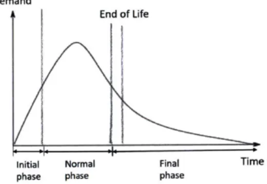
2. less accurate demand forecast due to sporadic and variable demands towards the end-of-life. Figure 1-1 shows the life cycle of a typical service part;
3. higher unit price due to smaller batch sizes [61.
Demand
End of Life
Initial Normal Final Time
phase phase phase
Figure 1-1: Service life cycle of a typical spare part [151
A highly responsive inventory system while minimizing the total cost is an oppor-tunity and a challenge for many OEMs [11].
Typically, companies increase the fulfillment rate of their service-parts supply chain operations by holding a large inventory at locations close to customer requests, which leads to high warehousing and inventory obsolescence costs, and capital costs tied to slow-moving parts
t91.
Now, the emergence of additive manufacturing (AM) technology creates an opportunity to manufacture service parts on demand to improve supply chain performance.1.3
Motivation
The intent of this research is to explore the economic implication and the best strat-egy of deploying additive manufacturing technology within a service-parts supply chain. The motivation of this project is two-fold. First, from the collaboration with a multinational automaker, we learned about their challenges in managing an end-of-life service-parts supply chain. Their suppliers are required to supply replacement and warranty parts for up to 10 years beyond the model year. The cost of storing tooling, and producing additional parts boosts the service part price. Moreover, these tools are often lost or damaged, causing service parts to have long lead times and sig-nificantly more cost to produce. Additively manufacturing service parts is projected to reduce production costs and lead time. However, it is not obvious how best to utilize the emerging capability to offset the comparatively higher production costs of additive manufacturing service parts. Some questions we are asked by the automaker include: for what types of parts would additive manufacturing be most valuable? Should 3D printing be a sole supplier of a part, or a dual supplier along with the original part supplier?
Additionally, research on the supply chain implications of additive manufacturing for service parts management is dominated by conceptual comparison with traditional manufacturing. As highlighted in the literature review, several papers quantitatively investigate the diverse operational aspects of additive manufacturing within service parts management
[18,
9, 51. However, most of these models make recommendation of one technology over the other to be implemented now given a demand forecast and cost parameters. But they do not have a holistic perspective on the life cycle of the service part. This thesis evaluates the supply chain strategies to be taken in the future given the uncertain timing of price increase in the life cycle of the service part.1.4
Current scenario
In the case of the automobile company, the demands of end-of-life service parts are typically low. Their inventory is currently replenished by issuing a material release to the primary supplier. After being packaged at a contract packaging supplier, the shipment is delivered to a warehouse and stored there until a dealer places an order, which is fulfilled by next day delivery.
The frequency of replenishment is determined by costs. Parts that cost more would be ordered more frequently to maintain a lower order quantity and a lower inventory level to avoid risking obsolescence of expensive parts. The timing of replenishment orders is determined by lead time since the replenishment order needs to arrive before inventory is depleted.
There are four lead times that are aggregated into the replenishment time used here.
o Supplier manufacturing lead time: time required by the supplier to manufacture the part
o Supplier to packager transportation lead time: time required to transport dock-to-dock from the supplier to the packager
o Packager lead time: time required by the packager to convert the bulk part into individually-packaged part
o Packager to warehouse lead time: time required to transport and process from packager to the warehouse
In general, low volume would be less than 400 pieces per year total sales to all dealers. Low volume parts on past models will typically have a manufacturing lead time from 60 to 90 days. A longer lead times makes the OEM carry more inventory and results in higher material release volatility. Later in the life of service parts, supply issues might arise, such as the supplier might lose the tooling, go out of business, or lose interest. In this case, the replenishment cost and lead time will increase
significantly or become infeasible and the automobile company has to obsolete the part, which is termed as non-policy obsolescence.
The main driver of additive manufacturing at this company is the non-policy obsolescence. Besides the supplier issues listed, other common reasons for non-policy obsolescence include:
" Supplier price increases and the company is unable to sell service parts at the elevated prices;
" Tooling needs to be replaced, but replacement tooling is too expensive;
" The old technology may be obsolete by the industry, such as electronic compo-nents.
The consequences of non-policy obsolescence are:
" Loss of goodwill from customers, especially if the dealer is not able to find an alternative to repair the customer's vehicle, such as using salvage or after-market part. It is hard to quantify customer dissatisfaction, but this can have an impact on their future purchase decisions.
* Loss of revenue from future lost sales.
" Potential loss of dealer purchase loyalty as the dealer has explored other sources for the service part that he may use in the future.
With additive manufacturing, the order from dealers would be fulfilled directly by 3D printing shops at the warehouse, which eliminates the need of holding a sig-nificant amount of inventory for sporadic demands. The traditional and additive manufacturing supply chain structures are compared in Figure 1-2.
waeose Dealer Supplier Wrhue Dealer
Figure 1-2: Comparing traditional (right) and additive manufacturing (left) supply chain structures
1.5
Thesis Outline
The remainder of this thesis is structured as follows. In Chapter 2, we provide on overview of the related literature on service parts inventory management and supply chain implication of additive manufacturing. In Chapter 3, we introduce the setup and assumptions for the two models for helping the automobile company decide the strategy with additive manufacturing capacity in the supply chain. In Chapter 4, we present the simulation results and sensitivity analysis. In Chapter 5, we demonstrate a robust optimization model to optimize the specifications in the model. Finally, we conclude in the last chapter.
Chapter 2
Literature Review
This thesis is related to two streams of literature: (i) service parts inventory manage-ment (ii) supply chain design for additive manufacturing. We discuss each stream in details below.
Service parts inventory management has been investigated extensively in the liter-ature. Sherbrooke first introduced METRIC, a mathematical model of a centralized supply chain system for repairable items
[16],
which was included in a review by Nah-mias in 1982 that summarizes the latest inventory systems for repairable service parts[14].
Kennedy et al[81,
Muckstadt[13]
and Basten and Van Houtum[2]
provide a more recent review on the inventory control for service parts. Many models find the optimal supply chain configuration for repairable parts by imposing system-oriented constraints, such as demand fill rate and expected number of shortage. In contrast, we analyze service parts that are available from multiple sources and not economically repairable and focus on minimizing the total supply chain cost.There are several analytical models in the operations management literature on the impact of 3D printing in the logistics supply chain. Song and Zhang [18] present a model that determines which parts should be printed and which should be stocked and the corresponding base-stock levels. Li et al
[12]
compare the total cost and carbon emissions of conventional supply chain, centralized additive manufacturing based supply chain and distributed additive manufacturing based supply chain using system dynamics simulation. They conclude that although AM-based supply chainhas lower total variable costs, it may not be more cost effective when fixed costs such as purchasing of 3D printers are taken into consideration. Khajavi et al
[9]
conduct scenario modeling of the service part supply chain for a F-18 Super Hornet fighter jet and find that distributed AM production is more favorable as AM machines become less expensive and more autonomous with shorter lead time. Heinen and Hoberg[5]
compare the related cost of traditional and additive manufacturing technologies for service parts and investigate the impact of warehouse locations. All of these mod-els have a strategic perspective to implement additive manufacturing within supply chains, but none of them characterizes the service parts most suitable for additive manufacturing.Chapter 3
Model Development
3.1
General setup
The initial application of additive manufacturing technology is primarily for service parts that are no longer used in vehicle production.
Towards the end of the product life cycle, the acquisition price can increase by more than 100%. One primary driver for the dramatic increase is because of the set up costs being amortized across a few pieces of the end product. The other reasons might include that the tools are lost or need repair or maintenance, the supplier is subject to a minimum subcomponent order quantity and the opportunity cost for the supplier. If the procurement cost is too high, the automaker may obsolete the part to avoid the risk of carrying service parts that probably will not sell at such an inflated price. In this case, the vehicle owner must find another option to secure a service part. However, for a low volume part, it is most likely that no after-market alternative exists, so a junk yard would become the only option, which is not ideal for most vehicle owners. Therefore, the automaker aspires to provide a high fulfillment rate and customer satisfaction level, even if it is unprofitable.
Sometimes, the supplier offers to produce one "last buy" when the automobile company's requested quantity cannot be produced for the current price on file. The automobile company may purchase a sufficient number of the end-of-life part to fulfill demands for its remaining life time if both parties can agree on the build quantity.
The supplier usually wants a larger quantity than the automobile company wants since the automaker does not like the risk of obsolescence. However, if the price increase is due to economic issue such as raw material cost increase, then there most likely would not be a last buy opportunity.
With additive manufacturing, the automaker has more options to maximize de-mand fill rate. This model evaluates the total cost of different end-of-life options. In building the model, we simplify the scenario of supplying low volume end-of-life parts as follows. As a service part approaches the end of life, its demand decreases and production cost increases. We assume that eventually, the primary supplier would in-crease the piece price dramatically and/or ask for an one-time fixed retooling charge. At this point, the automaker still desires to service the model requiring this part for a number of years and its goal is to minimize the total cost while maximizing the service level. The primary supplier does not give advanced notice for this change and the supplier may or may not offer a last buy opportunity, which poses a great challenge for end-of-life supply chain planning.
Figure 3-1 plots the demand forecast done in 2017 for an example part on a model that went out of production in 2001. The demand was predicted to drop to zero in 2034, which is 33 years after the model went out of production.
300 250--200 -150 100 -50 -0' 2018 2020 2022 2024 2026 2028 2030 2032 2034 Year
mine an OEM's best strategy in face of the price change and additive manufacturing capacity. In both models, we set the time period to be a year and we do not capture the within-year inventory replenishment dynamics because inventory is replenished at a different time scale. This assumption is made because OEM's demand forecast is done by year and the end-of-life strategy is reviewed every year.
We assume that the demand is stochastic and follows a Poisson distribution with mean of the yearly demand forecast, which is a common assumption in service parts management [17, 19]. From a network perspective, we model a single location with a centralized warehouse with additive manufacturing capacity. We assume that the investigated part meets the technical criteria to be printed and the technology is ready to be adopted anytime without delay. Additionally, any order placed with the primary supplier is subject to a minimum order quantity.
3.2
Model 1: unknown price change time
In this scenario, the service parts are being replenished from the primary supplier and we seek to understand the best strategy in presence of an uncertain timing of the price change. We are given the probability of a price change in each period (year) and the demand forecast for each year of the part's remaining life.
3.2.1
Evaluated strategies
When the supplier increases the per piece price and does not offer a last buy oppor-tunity, we evaluate the following strategies of OEM. They will be referred by their abbreviations later.
" obsoleting the part (obsolete)
When a price change happens, the OEM obsoletes the part and stops fulfill-ing customer demands after the inventory runs out. The total cost includes inventory holding cost and lost sales cost.
The OEM continues to replenish from the primary supplier at the inflated price. In each period, the OEM first orders an amount from the primary supplier, then a random demand is realized and the OEM fulfills customer demands. Since the order is placed before demand is observed, the order amount will be set to cover the demand with a high likelihood to avoid the stock-out risk. Specifically, the order amount is calculated as:
Order amt = forecast
+
safety factor x std dev. of the forecast - current inv. (3.1) A safety stock defined as any inventory ordered in excess of the forecast is main-tained for two reasons. First, accurately forecasting the demand for a service part is challenging and the observed demands usually deviate drastically from the forecast. Moreover, by building a safety stock when the unit resupply cost is lower, the OEM avoids replenishing at the elevated price at an undetermined time in the future. The total cost includes variable and fixed resupply cost and holding cost.e switching to additive manufacturing (print)
After the current inventory runs out, the OEM switches to AM and will fulfill the remaining customer demands by additive manufacturing. We assume that the replenishment lead time for AM resupply is relatively short, that is, on the order of a few weeks at most. We then assume that the OEM will hold a small safety stock so that the replenishment of parts will be nearly just in time. Thus, in each year, the OEM prints
Printing qty = demand -current inv. + safety stock, (3.2)
where the safety stock will be on the order of a few weeks of demand. The total cost includes variable and fixed additive manufacturing cost and holding cost. The total cost of every strategy includes holding cost which is computed by year and summed across the remaining lifetime of the product. The average of inventories
at the start and end of period is used to approximate the average inventory in this period. The holding cost in year i is computed as
start inv.
+
end inv.Holding cost = s x % of holding cost x Price in year i (3.3)
2
The last buy opportunity offered by the primary supplier gives the OEM two additional strategies that differ based on what the firm does after the last buy quantity has run out.
" obsoleting the part and incurring lost sales after last buy quantity runs out (LB - LS)
After last buy runs out, the OEM stops fulfilling customer demands and then incur lost sales. The total cost consists of last buy cost and lost sales cost. " additive manufacturing to fulfill demands after last buy quantity runs out (LB
- AM)
After last buy runs out, the OEM immediately starts printing the part to meet all future demands. The total cost consists of last buy cost and variable and fixed additive manufacturing cost
We assume that the primary supplier and the OEM can agree on a last buy quantity determined by the Newsvendor model. Let CAM denote the unit additive
manufacturing cost, CLB be the last buy unit price, CLS be the lost sales unit cost,
F be the cumulative distribution function of the remaining demand until end of life.
For LB - AM, the underage cost is CAM - CLB. For LB - LS, the underage cost is
CLS - CLB. The overage cost is CLB for both cases. Observe that with the AM option, we expect a lower underage cost, and thus a lower last buy quantity.
LB Qty for LB - AM = F_1 CAM - CLB - current inventory (3.4)
CAM
LB Qty for LB - LS = F_1 CLS - CLB - current inventory (3.5)
The uncertain time of the price change makes it difficult to obtain an analytical solution, and so the total costs and demand fill rates under different strategies are calculated by simulation. In the two options involving additive manufacturing, service parts are produced just-in-time for customer demands and thus, there are no stock-outs.
Different options are compared based on the total costs, which consist of
* resupply cost, including variable and fixed costs " last buy cost (if applicable)
" additive manufacturing cost (if applicable), including fixed and variable costs
" holding cost as percentage of the price calculated at the end of each period The inventory holding costs not only incorporate the physical space that the inventory takes up, but the opportunity cost of the capital tied up in inventory. " lost sales cost
The lost sales cost occurs when the company cannot meet customers' demand which diminishes customers' brand loyalty.
3.2.2
Assumptions
As noted earlier, we use one year as the time period, and we assume that with additive manufacturing, the production will effectively be just-in-time with a minimal safety stock to cover demand over the production lead time of a week or two. The additive manufacturing production times can range from 2 hours to 7 days per unit, but this time is not used in the simulation. To initiate additive manufacturing, we assume that there is no delay in implementing the technology, and there will be a fixed charge for development costs, such as purchasing of equipment.
For the simulation to be more realistic, we impose some assumptions on the cost parameters. Table 3.1 summarizes the notation for cost parameters in the model. We
Table 3.1: Cost parameters
Variable Notation
unit additive manufacturing cost CAM
Last buy unit price CLB
Lost sales unit cost CLS
The original price co
The elevated price after price change c1
assume that the CLS > cI > CAM > Co. The assumption CLS > CAM > co ensures
that additive manufacturing is economically more advantageous than obsoleting the part, but more expensive than purchasing directly from the primary supplier before the price change.
These assumptions on the unit cost do not make it immediately clear which option would be the least expensive after a price change. For example, although the lost sales unit cost is assumed to be greater than the increased price, obsoleting might be cheaper than resupplying at the increased price when not much demand is left after the price change. The lower volume and the fixed tooling charge from resupplying might justify the obsolescence option at the higher lost sales unit cost.
3.2.3
Simulation details
The simulation assumes a fixed time increment in which we simulate what happens each year, one year at a time, for the remainder of the part's life. Two random elements are realized each year: the demand for the year and whether or not there is a price change that year.
At the start of each year, a random demand is realized following Poisson distri-bution with its mean equal to the forecast. Additionally, a uniformly distributed number between 0 and 1 is generated as the price change signal. If it is less than the probability of price change, then the price will change in this period. Once the price changes, the increased price will be used in the calculation until the end of life.
The simulation model was built in Excel and each set of parameters was simulated 1000 times. The distribution and the average total cost for all strategies were recorded. Table 3.2 shows the demand forecast for the example part's life used in the base
case of simulation which are also plotted in Figure 3-1. Table 3.3 summarizes the additional variable values used.
Table 3.2: Demand forecast in the base example
Yr 1 2 3 4 5 6 7 8 9 10 11 12 13 14 15 16 17
D 265 274 250 198 154 118 89 66 49 25 18 13 9 6 4 2 0 Tot. 1539
Table 3.3: Input variable and values for unknown price change time model
Additive manufacturing unit cost $ 10
Price from the primary supplier before the price change $ 0.83
Last buy unit price $ 0.83
The increased price after the price change $ 20
Lost sales unit cost $ 30
Probability of price change in each year 15%
Safety factor 2
Minimum order quantity 100
Safety stock when AM is used 10
Holding cost (as a percentage of the price) 10% Fixed cost to transition to additive manufacturing $ 5000 Fixed cost to accept the price increase $ 5000
In the base example, we assume that the probability of price change is uniform across the part's lifetime. In reality, this probability should start low but grow over time as the demand declines. In the next chapter, we will present the simulation result when the probability of a price change varies year by year.
3.3
Model 2: current price change
This section presents a cost model for a different scenario in the service-parts supply chain. Many end-of-life parts in the automobile company expect a sequence of price changes as they progress towards the end of life. Their dilemma is to decide when to accept the price uplift, or obsolete the part, or switch to additive manufacturing given the forthcoming price increases.
To solve the company's dilemma, we model the following scenario. The primary supplier announces a price increase now, along with a tooling fixed charge. The OEM
also anticipates a second price change in the next few years and can estimate the probability of the second price change each year from now.
We evaluate the expected total cost during the remainder of the part As lifetime for different end-of-life strategies with additive manufacturing. The goal of this model is to help planners decide whether to switch to additive manufacturing in face of the first price change and forthcoming second price change based on the expected total cost.
The assumptions on unit cost for the simulation model for unknown price change still apply. The total cost consists of resupply cost, additive manufacturing cost and lost sales cost. In this analysis, we do not model the inventory holding cost as we expect it will be modest relative to the other costs.
3.3.1
Evaluated strategies
In face of the current price change and forthcoming second price change, the following strategies for the OEM are evaluated. They will be referred by abbreviations later.
If the primary supplier does not offer a last buy opportunity, the OEM may " switch to additive manufacturing now (AM now)
The demand is manufactured by AM in each period in a just-in-time fashion and the expected total cost includes variable and fixed additive manufacturing costs.
" accept the price increase and the fixed charge to continue with the supplier and switch to additive manufacturing at the second price change (AM at 2nd p
chg)
We order from the supplier between the first and second price change according to the forecast and will produce the demand in a just-in-time fashion with additive manufacturing after the second price change. The expected total cost includes variable and fixed resupply cost between the first and second price change and the variable and fixed additive manufacturing costs after the second price change.
If the primary supplier offers a last buy opportunity, in addition to the two options above, the OEM may
" make a last buy from the primary supplier and then switch to additive manu-facturing when the last buy quantity runs out (LB - AM)
Similar to the LB - AM option in the last model, the expected total cost consists of last buy cost and variable and fixed additive manufacturing costs.
" make a last buy and then obsolete the part when the last buy quantity runs out (LB - LS)
Similar to the LB - LS option in the last model, the expected total cost consists of last buy cost and lost sales costs.
The last buy quantities are determined by Newsvendor model (Equations 3.4 and 3.5) as in the model for uncertain price change time.
3.3.2
Inputs
The demand forecast in Table 3.2 was used in the base example of this model. Ta-ble 3.4 summarizes the additional variaTa-ble values used in the base example. Note that the fixed charge to transition to additive manufacturing is relatively inexpensive compared to the lost sales cost and additive manufacturing variable cost. Thus, the base example describes a futuristic scenario where additive manufacturing technology is more mature and less expensive. Also note that the base case assumes that there will be a second price change 4 years later and the probabilities of the second price in each of the subsequent four years are 0.1, 0.1, 0.4, 0.4.
3.3.3
Calculation of total cost
Last buyThe last buy quantities for LB - AM and LB - LS, denoted by qAM and qis, are determined with Equations 3.4 and 3.5 which are rewritten below, where Ic denotes the current inventory.
Table 3.4: Input variable and values for the current price change model
Expected total remaining demand 1539
Standard deviation of total remaining demand 38
Additive manufacturing unit cost $ 10
Fixed cost to transition to additive manufacturing $ 90
Last buy unit price $ 3
Minimum order quantity 100
The increased price after the first price change $ 5 Fixed cost to accept the price increase $ 270
Lost sales unit cost $ 40
Year between 1st and 2nd price changes 4 Probability of 2nd price change 1 year from now 0.1 Probability of 2nd price change 2 years from now 0.1 Probability of 2nd price change 3 years from now 0.4 Probability of 2nd price change 4 years from now 0.4
AM = F-1 CAM - CLB - Ic (3-6)
CAM
qLS = F 1
CLS - CLB - Ic (3.7)
CLS
In order to calculate the expected costs, we need to calculate the remaining de-mand after the last buy runs out. To do this, we will approximate the assumed Poisson demand of total remaining demand with normal distribution N(p, a). Then the
ex-pected number of shortages n(qAM) = ED[max(Demand-qAM-current inventory, 0)]
and n(qLS) after last buy runs out are computed using standardized loss function. The following equations demonstrate the calculation for n(qAM) and hold similarly
for
n(qLS)-The standardized loss function is defined as
L(z) =
(t
- z)#(t)dt (3.8) where#(t)
is the standardized normal density function. Let z = q^,* that is, z isstandard normal. Then it can be shown that
L(z) can be computed as
L(z) =
j
(t - z)o(t)dt = Let FAM denote the fixedn(qLS), the total cost of LB
-to(t)dt - z(1 - <b(z)) = O(z) - z(1 - 'D(z)) (3.10)
charge of transition to AM. After obtaining n(qAM) and -AM and LB - LS can be calculated as:
CLB-AM = (qAM - Ic)CLB + n(qAM)CAM + FAM (3.11)
(3.12) CLB-LS = (qLS - Ic)cLB + n(qLS)CLS
No last buy
For AM now, the customer demands are fulfilled in a just-in-time fashion. Thus, the number of additive manufactured parts is equal to the total demand, D, net the current inventory, I,, from the price change until the end of life.
CAMnow = (D - Ic) CAM + FAM (3.13)
For AM at 2nd price change, we first compute the expected demand between the first and second price change, Dbetw. Let pi be the probability that the second price
change happens in year i and Di be the demand in that year, i =1 ... n.
n i
(3.14)
E[Dbetw] = pi Dj
1 j=1
Then the remaining demand after the second price change, E[Dremain] is computed
as
E[Dremain] D - E[Dbtw] (3.15) Let c, denote the elevated price after price change. Let FtOO1 denote the fixed
charge to continue with the primary supplier after the first price change.
Chapter 4
Results and Discussion
This chapter presents the simulation results of the base cases for both models shown in the previous chapter. Using the base case result, we perform various sensitivity analyses to study the effect of individual parameter.
4.1
Model 1: unknown price change time
4.1.1
No last buy
As described in the previous chapter on Model Development, when the supplier in-creases the per piece price, we evaluate the following strategies of OEM if there is not last buy opportunity.
* obsoleting the part (obsolete)
When a price change happens, the OEM obsoletes the part and stops fulfilling customer demands after the inventory runs out.
" accepting the price increase and paying the fixed tooling charge (resupply) The OEM continues to replenish from the primary supplier at the inflated price. * switching to additive manufacturing (print)
After the current inventory runs out, the OEM switches to AM and will fulfill the remaining customer demands by additive manufacturing.
Each year, we simulate the random demand following Poisson distribution and the price change signal. Then we compute the inventory holding, lost sales, AM cost and purchasing cost. The total cost is obtained by summing across the cost in the part's entire lifetime. The demand fill rate is computed as:
demand fill rate = total demand - units of lost sales
total demand
Table 4.1 summarizes the additional variable values besides the demand forecast used.
Table 4.1: Input variable and values for unknown price change time model
Additive manufacturing unit cost $ 10
Price from the primary supplier before the price change $ 0.83
Last buy unit price $ 0.83
The increased price after the price change $ 20
Lost sales unit cost $ 30
Probability of price change in each year 15%
Safety factor 2
Minimum order quantity 100
Safety stock when AM is used 10
Holding cost (as a percentage of the price) 10% Fixed cost to transition to additive manufacturing $ 5000 Fixed cost to accept the price increase $ 5000
The first two columns of Table 4.2 present the average total cost and the average demand fill rate of 1000 simulated trials for the base case under the assumption that each strategy is implemented throughout the service part's lifetime, regardless whether it turn out to be the best strategy. The last column presents the percentage of 1000 trials where one particular strategy is the least expensive. Observe that the resupply strategy is never the best one even though the expected cost is lower than the obsolete strategy.
The random timing of price change makes it necessary to present the two eval-uation criteria: total cost and percentage of trials being the best strategy. Printing costs less than obsoleting and resupplying when the price change happens earlier in (4.1)
change happens later. This is because the volume of remaining demand is not high enough to justify the fixed charge for continuing with the supplier.
Due to the lack of concrete data, most of the model parameters are estimated. Thus, it is essential to perform a sensitivity analysis to understand the relative signif-icance of the parameters. The sections below explore the effect of other parameters.
Table 4.2: Base case
Strategy Expected Expected de- % trials that one total cost mand fill rate strategy costs the
$ least
Resupply 20285 99.91% 0%
Obsolete 20356 57% 36.5%
Print 12369 99.96% 63.5%
Changing the additive manufacturing cost
Currently, it takes $500,000 to $1,000,000 to purchase a commercial 3D printer, and the price is expected to drop as the additive manufacturing technology matures
[18].
Thus, we study the effect of simultaneously increasing the fixed and variable additive manufacturing costs on the expected total cost. Note that resupplying and obsoleting should be insensitive to the change in additive manufacturing cost.Table 4.3 presents the case of doubled fixed (10,000 instead of 5,000)and variable (20 instead of 10) additive manufacturing costs. Doubling the variable and fixed additive manufacturing cost almost doubles the expected total cost of printing and makes obsolescence the least-cost strategy in majority of all the trials. However, choosing the strategy of obsolescence also results in a lower demand fill rate.
Table 4.3: Doubled variable and fixed AM cost
Strategy Expected Expected de- % trials that one % change from the to-total cost mand fill rate strategy costs the tal cost in the base
$ least case
Resupply 20358 99.91% 43.3%
Obsolete 20356 57% 56.7%
Print 23663 99.95% 0%
t
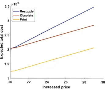
91%are increased by the same percentage while keeping all other parameters as in the base case. The advance of AM technology will change the variable and fixed costs of additive manufacturing simultaneously. We can see that switching to AM incurs the least cost when the AM unit cost is below $17 per piece.
2.6 x10⁴ -Resupply 2.4 -Obsolete - Print 2.2 -0 1.8 w 1.6 -1.4 1.2 10 12 14 16 18 20 22 AM unit cost
Figure 4-1: Plotting how the expected total cost changes with AM unit cost
Changing the part price
The base case describes a relatively inexpensive part, and we additionally examine what happens for a more expensive part. Table 4.4 shows the expected total cost and demand fill rate when the part originally costs $3.83 per piece instead of 0.83$ per piece and the supplier proposes $23 per piece instead of $20 per piece at the price change. Increasing the prices has the most impact on the resupply strategy.
Table 4.4: Increased prices before and after the price change
Strategy Expected Expected de- % trails that one % change from the total cost mand fill rate strategy costs the base case
$ least
Resupply 24487 99.91% 0%
t
20.7%Obsolete 22354 57% 36.9%
t
9.8%Print 14400 99.95% 63.1%
t
16.4%in the base case. Realistically, the increased price should be related directly to the original price. As shown in Figure 4-2, printing is strictly the best strategy in the range of prices examined. Obsoleting and switching to AM has the same sensitivity to the price and resupplying is more sensitive to the price, which is consistent with Table 4-2. This is because the resupply strategy purchases the more parts from the supplier than obsoleting and printing. Moreover, one of the obsoleting and printing strategies strictly dominates the other regardless of the price, depending on the lost sales unit cost.
3.5- X10 4 - Resupply -Obsolete 3 . -- Print 0 'R 2.5 40 0. V 1.5 1 20 22 24 26 28 30 Increased price
Figure 4-2: Plotting how the expected total cost changes with the increased price after price change
Changing the lost sales unit cost
The lost sales unit cost quantifies the lost revenue in the future if a unit of customer demand cannot be fulfilled now. Table 4.5 shows the expected total cost and demand fill rate when the lost sales unit cost is $35 instead of $30 as in the base case.
As shown in Table 4.5, the resupplying and printing strategies are barely sensitive to the lost sales unit cost. For obsoleting, as the lost sales unit cost increases, the expected total cost increases and fewer trials choose obsoleting as the least expensive strategy.
Table 4.5: Lost sales unit cost
Strategy Expected Expected de- % trails that one % change from the total cost mand fill rate strategy costs the base case
$ least
Resupply 20317 99.91% 0%
1
0.15%Obsolete 23662 57% 33.1%
4 5.8%
Print 12401 99.95% 66.9%
4 0.25%
When the lost sales case, resupply costs
unit cost is below $17, obsoleting costs the least. As in the base strictly more than printing, regardless of the lost sales unit cost.
2.6 2.4 2.2 0 2 0 1.8 1.6 C. X 1.4 1.2 - Resupply --Obsolete -- Print 15 20 25 30
Lost sales unit cost
35 40
Figure 4-3: Plotting how the expected total cost changes with lost sales unit cost
These sensitivity analyses show that the part price has little impact on the choice of strategy. The most favorable circumstance for additive manufacturing is when the lost sales unit cost is relatively high and the additive manufacturing cost is relatively low.
4.1.2
Last buy
If there is a last buy opportunity, the following strategies are evaluated:
* obsoleting the part and incurring lost sales after last buy quantity runs out (LB -Z
After last buy runs out, the OEM stops fulfilling customer demands and then incur lost sales.
* additive manufacturing to fulfill demands after last buy quantity runs out (LB - AM)
After last buy runs out, the OEM immediately starts printing the part to meet all future demands.
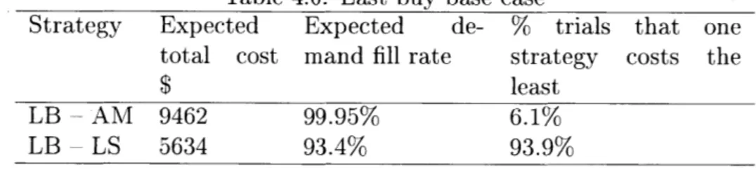
Table 4.6: Last buy base case
Strategy Expected Expected de- % trials that one total cost mand fill rate strategy costs the
$ least
LB - AM 9462 99.95% 6.1%
LB LS 5634 93.4% 93.9%
Table 4.6 shows the average total cost and demand fill rate of 1000 trials in the simulation for the base case involving last buy opportunity. In 939 out of the 1000 trials, obsoleting after the current inventory runs out costs the least while maintaining 93% demand fill rate. Using the result of the base case, we explore the effect of other parameters below.
Changing lost sales unit cost
As shown in Figure 4-4, the LB-AM strategy is barely sensitive to the lost sales unit cost and the additive manufacturing only becomes the better strategy when lost sales unit cost becomes greater than $60.
Changing last buy price
Figure 4-5 plots how the expected total cost changes with the last buy price. Last buy price above $10 was not examined because it would violate the assumption that the last buy price should be less than the unit print cost ($10). The LB-LS strategy results in a higher last buy quantity than LB-AM strategy because LB-LS strategy has a higher underage cost. Thus, the total cost of LB-LS is more sensitive to the
0 0. -W 10000 9500 9000 8500 8000 7500 7000 6500 -- LB-LS -LB-AM 30 35 40 45 50 55 60 65
Lost sales unit cost
Figure 4-4: Plotting how the expected total cost changes with lost sales unit cost in presence of last buy opportunity
last buy price and LB-AM would be the better strategy when the last buy price is sufficiently high. 2.5 0 0 LU 2 -X10A4 1.5 [ 0.5 1' ' 0 2 4 6
Last buy price
8 10
Figure 4-5: Plotting how the expected total cost presence of last buy opportunity
changes with lost sales unit cost in
Having a last buy opportunity not only drops the total cost significantly, but also diminishes the value of additive manufacturing. In the base case, the total cost of LB-LS is 40.4% lower than LB-AM only with a slightly lower demand fill rate (93%
- L-D-iLa
last buy price are sufficiently large.
4.1.3
Increasing probability of price change
One parameter in the simulation model for unknown price change time is the probabil-ity of price change every year. In the base case described in Table 3.3, the probabilprobabil-ity of price change is 15% every year. In reality, the probability of price change increases as the model is out of production for longer. Therefore, we investigate the cases where the probability of price change increases linearly and quadratically with the number of period.
For linearly increasing probability of price change, the probability of price change in period i, pi, increases from 7% in period 1 to 15% in period 17.
pi = 6.5% + 0.5%i (4.2)
For the quadratic case, pi increases from 2.2% in period 1 to 15% in period 17.
pi = 15% - (17 - i)20.05% (4.3)
Table 4.7: Linearly increasing probability of price change Strategy Expected total cost $ Demand fill rate
Resupply 14701 99.92%
Obsolete 13086 74.07%
Print 9657 99.94%
LB - AM 7993 99.94%
LB - LS 4770 96.04%
Table 4.8: Quadratically increasing probability of price change Strategy Expected total cost $ Demand fill rate
Resupply 11844 99.92%
Obsolete 9159 82.8%
Print 8298 99.93%
LB - AM 7291 99.93%
Comparing Table 4.7 and 4.8 with Table 4.2, the expected total costs for non-uniform probability of price change are lower for all strategies. The demand fill rate for the obsoleting strategy increases by 27.8% than the case of uniform price change probability. Comparing Table 4.7 with Table 4.8, a more dramatic change in the probability of price change reduces further the total costs for all strategies.
4.2
Model 2: current price change
Recall that in this model, we assume that there is a price change now. This model eval-uates the expected total cost in order to help supply chain planners decide whether to switch to additive manufacturing in face of the current price change and forthcoming second price change.
4.2.1
No last buy
If the primary supplier does not offer a last buy opportunity, we evaluate the following strategies of OEM:
" switch to additive manufacturing now (AM now)
The demand is additive manufactured in each period in a just-in-time fashion.
" accept the price increase and the fixed charge to continue with the supplier and switch to additive manufacturing at the second price change (AM at 2nd p chg)
We order from the supplier between the first and second price change according to the forecast and will produce the demand in a just-in-time fashion with additive manufacturing after the second price change.
Since both strategies entail just-in-time production, the demand fill rate is 100% and omitted in the comparison.
Table 4.9: Base case for the current price change model Strategy Expected total cost $
AM now 14480 AM at 2nd price change 14399 3 x10 4 I-AM-AM 2.5 2 U 0 0-now after 2nd p chg 1.5 F 5 10
Unit print cost C
15 20
Figure 4-6: Plotting how the expected total cost changes with AM unit cost in face of the current price change and forthcoming 2nd price change
Changing the additive manufacturing cost
We performed sensitivity analysis on the total cost with respect to the unit print cost. When there is no last buy opportunity, it is more economical to continue with the current supplier and switch to AM after the expected second price change occurs as unit print cost increases above $11. The total cost for the AM now strategy increases faster with respect to the unit print cost because more units are additively manufactured.
4.2.2
Last buy
If the primary supplier offers a last buy opportunity, the OEM additionally may
e make a last buy from the primary supplier and then switch to additive manu-facturing when the last buy quantity runs out (LB - AM)
I
-0.5