Benchmark tests based on the Couette viscometer

HAL Id: hal-01667115

https://hal.archives-ouvertes.fr/hal-01667115

Submitted on 11 Oct 2018

HAL is a multi-disciplinary open access

archive for the deposit and dissemination of

sci-entific research documents, whether they are

pub-lished or not. The documents may come from

teaching and research institutions in France or

abroad, or from public or private research centers.

L’archive ouverte pluridisciplinaire HAL, est

destinée au dépôt et à la diffusion de documents

scientifiques de niveau recherche, publiés ou non,

émanant des établissements d’enseignement et de

recherche français ou étrangers, des laboratoires

publics ou privés.

Distributed under a Creative Commons Attribution| 4.0 International License

Benchmark tests based on the Couette viscometer

Thomas Heuzé, Hussein Amin El Sayed, Jean-baptiste Leblond, Jean-michel

Bergheau

To cite this version:

Thomas Heuzé, Hussein Amin El Sayed, Jean-baptiste Leblond, Jean-michel Bergheau.

Bench-mark tests based on the Couette viscometer: II: Thermo-elasto-plastic solid behaviour in small and

large strains. Computers & Mathematics with Applications, Elsevier, 2014, 67 (8), pp.1482-1496.

�10.1016/j.camwa.2014.02.010�. �hal-01667115�

Benchmark tests based on the Couette viscometer—II:

Thermo-elasto-plastic solid behaviour in small and

large strains

Thomas Heuzé

a,∗

_{, Hussein Amin-El-Sayed}

b

_{, Jean-Baptiste Leblond}

c

_,

Jean-Michel Bergheau

b

a_{Research Institute in Civil and Mechanical Engineering (GeM, UMR 6183 CNRS), École Centrale de Nantes, 1 rue de la Noë,}

F-44321 Nantes, France

b_{Université de Lyon, ENISE, LTDS, UMR 5513 CNRS, 58 rue Jean Parot, 42023 Saint-Etienne, Cedex 2, France}

c_{Institut Jean Le Rond d’Alembert, Université Pierre et Marie Curie-Paris 6, UMR CNRS 7190, 4 Place Jussieu Tour 55-65, 75252 Paris,}

Cedex 05, France

The Couette viscometer is a well-known problem of fluid mechanics, well-suited for the verification of numerical methods. The aim of this work is to extend the classical steady state mechanical solution obtained in fluid mechanics and to use the extended solutions to assess new finite elements. Part I was devoted to the case of laminar flow of incompressible fluids with inertia effects and thermomechanical coupling. The present Part II focuses on solid-type nonlinear behaviours; we address the cases of elastic–plastic and thermo-elastic–plastic von Mises materials, both in small and large strains. The extended solutions permit to assess a new formulation of a mixed P1 + /P1 finite element in solid mechanics, in a temperature/velocity/pressure formulation coupled with an implicit (backward) Euler algorithm in time. The verification evidences a good behaviour of the solid finite element.

1. Introduction

Part I was devoted to the viscometer problem in the case of fluid-type behaviours; extended solutions were defined accounting for inertia effects and strong coupling between thermal and mechanical effects. Though the viscometer is generally considered as a typical fluid mechanics apparatus or problem, it seems natural to keep the same problem to develop benchmark tests for solid-type nonlinear behaviours. Extensions of the problem to solid materials are therefore the topic of the present Part II.

In Section2, we consider the case of an elastic–plastic material obeying the von Mises criterion with isotropic hardening. The elastic–plastic problem is first studied in Section2.1in the small strain framework. It is shown that the displacement field is found by integrating a function defined by the elastic–plastic constitutive law. The load curve of the structure and the unloading stage are then studied in Sections2.3and2.4. It is shown that for the Couette viscometer the unloading leads, somewhat surprisingly, to a vanishing residual stress field. An extension to the large strain framework is then presented in Section2.5.

∗_{Corresponding author.}

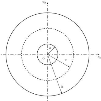
Fig. 1. Parameterization of the Couette viscometer problem.

In Section3, the Couette viscometer problem is addressed in thermo-elasto-plasticity. The solution permits to account for the generation of heat through plastic dissipation within the structure. The solution developed is valid only during the phase when the structure is entirely elastic–plastic.

The purpose of the extension of the Couette viscometer problem to solid behaviours is to assess a formulation in solid mechanics of the P1

+

/

P1 finite element initially introduced by Arnold et al. [1]. This element is developed in Section4in a new, fully coupled temperature/velocity/pressure formulation in the large strain framework, combined with an implicit (backward) Euler algorithm in time. The bubble node embedded in this element enables to ensure, with the mixed formulation, plastic incompressibility. The resolution is performed on the unknown configuration at time t

+

1t. This element is one feature of the modelling of the Friction Stir Spot Welding process [2] recently implemented in the finite element code SYSWELD⃝R

[3].

The verification of the solid P1

+

/

P1 finite element is subsequently performed using the reference solutions developed, and presented in Section5. First, the mechanical behaviour of the finite element is tested with respect to the solution developed in Section2.5in the large strain framework. The comparison shows a good agreement between numerical and analytical solutions. Second, the thermomechanical behaviour of the finite element is tested with respect to the solution developed in Section3. Comparisons on thermal and mechanical fields also show a good agreement between numerical and analytical solutions.

2. The Couette viscometer problem for an elastic–plastic von Mises material with strain hardening 2.1. Small strain framework

We consider the Couette viscometer problem schematized inFig. 1. The inner and outer cylinder radii are denoted a and b respectively. We shall consider in the sequel the inner cylinder as fixed and the outer cylinder as driven:

u_θ

(

r

=

a

) =

0

u_θ

(

r

=

b

) =

u_θ

(

b

)

(1)

where u_θdenotes the orthoradial displacement. The aim of this choice, which differs from that made in Part I for fluid-type behaviours, is to warrant a positive shear stress

σ

rθ

≡

τ

.

We consider in this section an elastic–plastic material obeying a von Mises criterion with isotropic hardening. The yield stress is supposed not to saturate, that is to increase indefinitely with the plastic strain. The study is performed in the small strain framework with an increasing monotonic loading, starting from a natural initial state. Since an elastic–plastic constitutive law is used, three regimes occur during the loading:

•

the fully elastic regime: the structure deforms elastically.

•

the mixed elastic–plastic/elastic regime: an elastic–plastic crown appears adjacent to the inner radius, surrounded by an elastic crown.

Fig. 2. Elastic–plastic crown radius c in the mixed elastic–plastic/elastic regime.

The stress field within the structure is of the form:

σ = τ(

er

⊗

eθ

+

eθ

⊗

er

)

(2)

where

σ

denotes the Cauchy stress tensor and

τ

a shear stress component. The tangential equilibrium equation: d

τ

dr

+

2

τ

r

=

0 (3)

implies that this shear stress must be of the form:

τ =

A

r2 (4)

where A is a constant which can be determined from appropriate boundary conditions. This constant may be rewritten as:

A

=

kc2 (5)

leading to the following expression of the shear stress:

τ =

kc

2

r2 (6)

where k is the initial shear yield stress and c a parameter homogeneous to a length, which can serve as a loading parameter. Plasticity occurs at a given point r if

τ ≥

k or equivalently c

≥

r. Thus, it follows that if:

•

c

<

a, the structure is completely elastic,

•

a

≤

c

<

b, the structure is in a mixed elastic–plastic/elastic regime,

•

c

≥

b, the structure is completely elastic–plastic.

In the second case, the constant c denotes the radius of the inner elastic–plastic crown, as shown inFig. 2.

It remains to calculate the displacement field to complete the solution. This will be done by using the following equations:

τ =

kc 2 r2 (equilibrium)

τ =

f

(γ )

(constitutive law)

γ =

2

ε

rθ

=

du_θ dr

−

u_θ r (definition of strain)

.

(7)

The function f

(γ )

appearing in Eq.(7)2is supposed to be strictly increasing.

The constitutive law(7)2combined with the expression(7)1of the stress permits to express the strain as a function of the load parameter c:

γ =

f−1



kc 2 r2



≡

g



r c



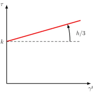
(8)

Fig. 3. Strain hardening law.

where g is a function defined from the inverse of f . The definition(7)3of the strain implies that:

γ =

duθ dr

−

u_θ r

=

r d dr



u_θ r



=

g



r c

 .

(9)

Thus, the displacement field is obtained through integration: u_θ

(

r

) =

r



r a g

(

r′

/

c

)

r′ dr ′

_.

(10) The displacement of the outer cylinder u_θ

(

b

)

is therefore given by:

u_θ

(

b

) =

b



b a g

(

r′

_/

_c

₎

r′ dr ′

_.

(11) It is worth noting that u_θ

(

b

)

can be explicitly expressed as a function of c, whereas the converse is not true. This justifies the choice of c rather than u_θ

(

b

)

as a load parameter.

2.2. Specialization of the solution

The general solution for the displacement field is given by Eq.(10), provided that the function g is defined from an increasing function f . It is interesting to specialize this solution to a given constitutive law in order to derive an explicit expression of the displacement field, allowing for a comparison between numerical and analytical solutions. We shall consider a linear hardening law in the sequel, seeFig. 3.

Explicit expressions of the displacement field will be derived for each regime occurring during the monotonic loading of the structure.

2.2.1. Fully elastic regime (c

<

a)

In the linear regime, the function g is noted geand is defined by: ge



r c



=

γ =

τ(

r

)

G

=

k G c2 r2 (12)

where G denotes the elastic shear modulus. This leads upon calculation of the integral of Eq.(10)to:

u_θ

(

r

) =

kr 2G c2 a2



1

−

a 2 r2



.

(13)

In particular, the parameter u_θ

(

b

)

is related to c through the relation: u_θ

(

b

) =

kb 2G c2 a2



1

−

a 2 b2



.

(14)

2.2.2. Mixed elastic–plastic/elastic regime (a

≤

c

<

b)

In the mixed elastic–plastic/elastic regime, an elastic–plastic crown is surrounded by an elastic crown, thus the calculation of the integral(10)is performed separately in these two zones.

Elastic–plastic zone

Since the initial state is supposed to be stress-free and the loading monotonically increasing, the elasticity law, the von Mises criterion and the expression of the cumulated plastic strain

ε

eqread:























τ =

G

(γ − γ

p

)

τ =

k

+

h

√

ε

eq 3

ε

eq

=

γ

p

√

3 (15)

where h denotes the strain hardening parameter in simple tension. Elimination of

γ

p_and

_ε

eqin Eqs.(15)gives:

γ =

h

+

3G

hG

τ −

3k

h

.

(16)

Introducing Eq.(16)into(10), one gets the displacement field within the elastic–plastic zone:

u_θ

(

r

) =

kr



h

+

3G hG c2

₍

_r2

₋

_a2

₎

2a2_r2

−

3 hln



r a





.

(17)

The cumulated plastic strain is in turn obtained by combining Eqs.(15)2and(6):

ε

eq

(

r

) =

√

3k h



c2 r2

−

1



.

(18) Elastic zone

The elastic crown surrounds the elastic–plastic one, therefore the integral in Eq.(10)must be split in two to account for both the elastic–plastic and elastic zones:

u_θ

(

r

) =

r



c a gp

₍

_r′

_/

_c

₎

r′ dr ′

₊



r c ge

₍

_r′

_/

_c

₎

r′ dr ′



(19) where g takes the following expressions, noted geand gpin the elastic and elastic–plastic zones respectively:

∗

ge

(

r′

/

c

) =

k G c2 r′2 for c

≤

r ′

_≤

r

,

(20)

∗

gp

(

r′

/

c

) =

h

+

3G hG

τ(

r ′

_{) −}

3k h for a

≤

r ′

_≤

c

.

(21)

The calculation of the integrals provides the following solution:

u_θ

(

r

) =

kr



h

+

3G hG c2

₋

_a2 2a2

−

3 hln



c a



+

1 2G



1

−

c 2 r2



.

(22)

In particular, the parameter u_θ

(

b

)

can be expressed as a function of the plastic crown radius c: u_θ

(

b

) =

kb



h

+

3G hG c2

−

a2 2a2

−

3 hln



c a



+

1 2G



1

−

c 2 b2



.

(23)

2.2.3. Fully elastic–plastic regime (c

≥

b)

When the whole structure is elastic–plastic, the sole function gpappears in the integral(10), thus the expression of the displacement field is given by(17). In particular, the parameter u_θ

(

b

)

is connected to the radius c by the relation:

u_θ

(

b

) =

kb



h

+

3G hG c2 2a2



1

−

a 2 b2



−

3 hln



b a



.

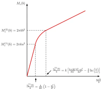
(24)

Fig. 4. Load–displacement curve of the structure.

2.3. Load–displacement curve of the structure

Dual force and displacement parameters Q, q can be defined in such a way that the power of external forces read:

Pext

=

Q

· ˙

q

.

(25)

In the case of the Couette viscometer with the loading considered, these parameters may be identified as: Q

=

Mz

(

b

)

q

=

uθ

(

b

)

b

(26)

where the torque per unit thickness Mz

(

b

)

is defined as: Mz

(

b

) =

M

(

O

) ·

z

=



ber

×

(σ ·

er

)

bd

θ



·

z

=

2

π

b2

τ(

b

).

(27) This torque can be calculated for each regime occurring during the loading:

•

fully elastic regime

Combining formulae(12)–(14)and(27), one gets:

Mz

(

b

) =

4

π

Ga2_b2

b2

₋

_a2

u_θ

(

b

)

b (28)

•

mixed elastic–plastic/elastic regime One gets similarly:

Mz

(

b

) =

2

π

kc2 (29)

where c is a function of u_θ

(

b

)

defined implicitly by relation(23).

•

fully elastic–plastic regime

The plastic crown radius c is given here by(24), thus the expression of the torque reads:

Mz

(

b

) =

4

π

ka2_b2 b2

₋

_a2 hG h

+

3G



u_θ

(

b

)

kb

+

3 hln



b a



.

(30)

The load–displacement curve of the structure is shown inFig. 4. The structure remains completely elastic up to the load of incipient plasticity Mz(1)

(

b

)

. Subsequently, a plastic crown gradually develops from the inner cylinder and extends radially

until the whole structure becomes elastic–plastic, for the second torque Mz(2)

(

b

)

. Afterwards, the torque increases linearly

2.4. Unloading

It is interesting to study an unloading of the structure from some completely elastic–plastic state and calculate residual stresses. The unloading leads to a zero force parameter Q. In the case of the Couette viscometer, the torque on the outer cylinder thus goes to zero, and so does also the shear stress at r

=

b. But it has been shown using the equilibrium equation

(7)₁that the shear stress varies as 1

/

r2. Therefore, the residual shear stress vanishes over the whole structure when it is unloaded. This property is of course tied to the special nature of the problem considered and by no means general. More precisely, the plastic strain field is always of the form

ε

_rp_θ

=

γ

p

(

r

)/

2, other

ε

p_ij

=

0. Such a strain field is always compatible, because the differential equationdu

p θ dr

−

up_θ r

=

γ

p

₍

_r

₎

_{(where u}p

θis some unknown ‘‘plastic displacement’’) always admits a solution; it is a well-known property of plasticity theory that the residual stresses after unloading are then necessarily zero [4,5].

2.5. Extension to the large strain framework

The Couette viscometer problem for an elastic–plastic material has been considered in the small strain assumption up to now. Its extension to the large strain framework is important for the assessment of a new formulation of the P1

+

/

P1 finite element presented in Section4.

The plasticity equations in large strain are written here in the Eulerian form; the linearized strain rate tensor

ε

˙

is replaced by the Eulerian strain rate tensor D. The latter tensor is decomposed additively into elastic and plastic parts De

_,

_Dp_{. The elastic}

strain rate tensor Deis linked to an objective stress rate through some hypoelastic law, while the plastic strain rate tensor Dp_{is given by the flow rule associated to von Mises’s criterion.}

The presence of some objective derivative of the stress tensor in the hypoelastic law makes the solution more complex. However, if the additional terms associated to this objective derivative are neglected, the solution developed for small strains remains unchanged provided the tangential displacement u_θ is replaced by the curved arc length swept l. This point is detailed in theAppendix.

3. The Couette viscometer problem in thermo-elasto-plasticity

We develop in this section a solution of the Couette viscometer problem in thermo-elasto-plasticity, accounting for the generation of heat through plastic dissipation within the structure. This solution allows for comparisons with the P1

+

/

P1 solid finite element developed with a strong thermomechanical coupling presented in Section4. The mechanical part of the solution corresponds to an elastic–plastic constitutive law with the von Mises criterion and a linear isotropic strain hardening (Fig. 3), already considered in both small and large strain in Section2. The thermal part of the solution is governed by the equation of energy conservation:

ρ

C

∂

T

∂

t

=

∇ ·

(λ∇

T

) +

S

∀

x

∈

Ω (31) supplemented with appropriate initial and boundary conditions. The parameters

ρ,

C and

λ

here denote the density, the heat capacity and the thermal conductivity, respectively, and S is a source term. The kinematics of the Couette viscometer permit to simplify Eq.(31)into:

ρ

C

∂

T

∂

t

=

λ

r

∂

∂

r



r

∂

T

∂

r



+

S

.

(32)

The strong thermomechanical coupling consists on the one hand of the effects of the mechanical dissipation appearing in Eqs.(31)and(32)in the source term S, and on the other hand of thermal dilation and temperature dependent mechanical parameters. To facilitate the solution, the influence of the thermal part of the solution upon its mechanical part is not accounted for here, that is dilation effects are neglected and mechanical material parameters are fixed, independently of temperature.

With these assumptions, the mechanical dissipation is given by:

S

=

βτ ˙γ

p (33)

where

β

denotes the Quinney–Taylor coefficient accounting for the fact that only a portion of the plastic power is dissipated into heat; this coefficient is usually set to 0.9. The mechanical dissipation S is here time-dependent, thus the thermal part of the solution depends on its mechanical part determined a priori. Assuming the structure to be entirely elastic–plastic, the shear stress

τ

is given by Eq.(6)and the plastic rate of slip

γ

˙

pby the expression 3

τ/

˙

h resulting from Eqs.(15)2and(15)3; the mechanical dissipation can then be expressed as:

S

=

6

β

k

2

h c3_c

_˙

To solve the partial differential equation(32), it is convenient to assume that both the plastic crown radius c and the temperature vary exponentially in time, in order to allow for a separation of space and time coordinates. Let the evolution of the plastic crown radius be thus given by:

c

(

t

) =

c0exp

(α

t

)

(35)

where

α

is a constant homogeneous to the inverse of a time. The mechanical dissipation is then expressed as: S

=

6

β

k 2_c4 0

α

h exp

(

4

α

t

)

r4

.

(36)

The temperature is now assumed to be of the form:

T

(

r

,

t

) =

f

(

r

)

exp

(

4

α

t

).

(37)

The partial differential equation (32)reduces to the following inhomogeneous ordinary differential equation on the unknown function f

(

r

)

: f′′

(

r

) +

f ′

₍

r

)

r

−

µ

2_f

₍

_r

_{) = −}

6

β

k2c 4 0

α

h

λ

1 r4 where

µ

2

₌

4

ρ

C

α

λ

.

(38)

To solve Eq.(38), we first perform a change of variable and function:

x

=

µ

r

,

F

(

x

) =

f

(

r

)

(39)

where since x is dimensionless,

µ

is homogeneous to the inverse of a length. Eq.(38)can be rewritten, accounting for(39), as: F′′

(

x

) +

F ′

₍

_x

₎

x

−

F

(

x

) = −

B x4 (40)

where B is a constant defined by: B

=

6

β

k

2_c4 0

αµ

2

h

λ

.

(41)

Eq.(40)can be identified to a modified inhomogeneous Bessel’s equation [6] at order zero. We look for a solution of Eq.(40)in the form:

F

(

x

) =

I0

(

x

)

G

(

x

)

(42)

where I0

(

x

)

is the modified Bessel function of the first kind at order zero, and G

(

x

)

an unknown function. Introducing(42) into(40), and noting that I0

(

x

)

satisfies the homogeneous equation associated to(40), one gets:

G′′

(

x

) +



1 x

+

2I₀′

(

x

)

I0

(

x

)



G′

(

x

) = −

B I0

(

x

)

x4

.

(43) By setting H

(

x

) =

G′

(

x

)

, Eq.(40)is reduced to the first order differential equation

H′

(

x

) +



1 x

+

2I′ 0

(

x

)

I0

(

x

)



H

(

x

) = −

B I0

(

x

)

x4

.

(44) The solution of the homogeneous equation associated to(44)is obtained through separation of variables and is given by:

H

(

x

) =

K xI2

0

(

x

)

(45) where K is a constant. The method of variation of the constant then permits to determine the solutions of Eq.(44); one thus finds that:

H

(

x

) =

B

φ(

x

) −

C1 xI2

0

(

x

)

(46) where C1is a constant and the function

φ(

x

)

is defined by:

φ(

x

) =



s x

I0

(

u

)

The upper bound s of the integral defining

φ(

x

)

may be set arbitrarily (changing it just changes the value of the constant C1). However, since the integrand of

φ(

x

)

goes to infinity for u

→ +∞

,

s should be ascribed some finite value.

To calculate the function G

(

x

)

, the expression(46)of the function H

(

x

)

needs to be integrated. Use will be made here of the following identity which can be established by combining formulas 9.6.15 and 9.6.27 of Abramowitz and Stegun [7]:



K0 I0



′

(

x

) = −

1 xI₀2

(

x

)

(48)

where K0

(

x

)

is the modified Bessel function of the second kind at order zero. According to Eq.(48), the expression of H

(

x

)

may be written in the form:

H

(

x

) = (−

B

φ(

x

) +

C1

)



K0 I0



′

(

x

).

(49)

The function G

(

x

)

is then obtained through integration. The second term of Eq.(49)is directly integrated whereas the first one is integrated by parts. The solution of Eq.(40)finally reads:

F

(

x

) = (

C₂

+

B

ψ(

x

))

I₀

(

x

) + (

C₁

−

B

φ(

x

))

K₀

(

x

)

(50) where C2is an additional constant and the function

ψ(

x

)

is defined by:

ψ(

x

) =



+∞

x

K0

(

u

)

u3 du

∀

x

>

0

.

(51)

Taking an infinite upper bound here does not raise any problem since K0

(

u

)

goes to zero when u goes to infinity.

Boundary conditions are defined in such a way as to lead to the simplest possible expression of the solution field. We thus prescribe homogeneous Dirichlet conditions on both cylinders:



T

(

r

=

a

,

t

) =

0

⇒

f

(

a

) =

0

⇒

F

(µ

a

) =

0

T

(

r

=

b

,

t

) =

0

⇒

f

(

b

) =

0

⇒

F

(µ

b

) =

0

.

(52)

Note that other couples of boundary conditions, such as zero fluxes imposed on the cylinders, could also be prescribed. Solving the system of Eqs.(52)leads to the following values of the constants C1and C2:

C1

=

B [

−

I0

(µ

a

)

K0

(µ

b

)φ(µ

b

) +

I0

(µ

b

)(

K0

(µ

a

)φ(µ

a

) −

I0

(µ

a

)(ψ(µ

a

) − ψ(µ

b

)))

] I0

(µ

b

)

K0

(µ

a

) −

I0

(µ

a

)

K0

(µ

b

)

C₂

=

B [

−

I0

(µ

a

)

K0

(µ

b

)ψ(µ

a

) +

K0

(µ

a

)(

K0

(µ

b

)(φ(µ

a

) − φ(µ

b

)) +

I0

(µ

b

)ψ(µ

b

))

] I0

(µ

a

)

K0

(µ

b

) −

I0

(µ

b

)

K0

(µ

a

)

.

(53)

Therefore the transient temperature field in the coupled thermo-elasto-plastic viscometer problem is given by: T

(

r

,

t

) =

[

(

C2

+

B

ψ(µ

r

))

I0

(µ

r

) + (

C1

−

B

φ(µ

r

))

K0

(µ

r

)

] exp

(

4

α

t

)

with

α =

λµ

2 4

ρ

C

(µ

arbitrary parameter

)

B

=

6βk 2_c4 0αµ2 hλ

,

C1

,

C2given by (53)

, φ(

x

)

by (47)

, ψ(

x

)

by (51) T

(

r

=

a

,

t

) =

0 T

(

r

=

b

,

t

) =

0 T

(

r

,

t

=

0

) =

T0

(

r

).

(54)

4. Mixed temperature/velocity/pressure formulation for the P1

+

/

P1 solid finite element

4.1. Weak formulation

In welding applications, geometrical nonlinearities such as large rotations often occur, and govern the deformed shape of the structure [8–16]. Moreover, certain welding processes such as Friction Stir Welding also involve large strains [17,18]. In addition, Friction Stir Welding involves a strong coupling between thermal and mechanical effects. Indeed, the heat generated by friction and the motion of the material generates a mix which joins the parts to be welded after cooling. We propose a special formulation in solid mechanics within the large displacement/strain framework (Eulerian setting) which includes a strong thermomechanical coupling. We shall assume that the boundary

∂

Ωof the domainΩadmits the

decompositions

∂

Ω

=

∂

Ω_v

∪

∂

Ω_F

∅ =

∂

Ω_v

∩

∂

Ω_F (55)

∂

Ω

=

∂

Ω_θ

∪

∂

Ω_q

∅ =

∂

Ω_θ

∩

∂

Ω_q (56) where

∂

Ω_vand

∂

ΩF are respectively these parts of the boundary on which the velocities and tractions are prescribed, and

∂

Ωθand

∂

Ωqthose on which the temperature and the heat flux are prescribed.

In a mixed formulation, the weak form of the problem is as follows: given the body forces f, the heat source r, the prescribed tractions Fdon

∂

ΩF, and the prescribed thermal flux

φ

don

∂

Ωq, plus some initial conditions T0

(

x

),

v0

(

x

)

,

(

W

)























































Find

(

T

,

v

,

p

) ∈ (

Tad

×

Vad

×

Pad

), ∀

t

∈ [

0

,

T

]

,

such that

∀

(

T ∗

_,

v∗

,

p∗

) ∈ (

Tad0

×

Vad0

×

Pad

),

























−



Ω k

∇

T

·

∇

T∗dΩ

+



∂Ωq

φ

d_T∗ dS

+



Ω

βσ :

DpT∗dΩ

+



Ω r T∗dΩ

=



Ω

ρ

C

∂

T

∂

tT ∗ dΩ

−



Ω

σ :

D∗dΩ

+



∂ΩF Fd

·

v∗dS

+



Ω f

·

v∗dΩ

=

0



Ω p∗trDpdΩ

=

0 T

(

x

,

t

=

0

) =

T0

(

x

)

v

(

x

,

t

=

0

) =

v0

(

x

)

(57)

where

β

denotes the Quinney–Taylor coefficient introduced in Section3, and Dp_{the plastic part of the strain rate. The}

functional spaces involved here are defined as

Vad

= {

v

(

x

,

t

) ∈ [

H1

(

Ω

)]

3

|

v

(

x

,

t

) =

vd

(

x

,

t

)

on

∂

Ωv

}

V_ad0

= {

v∗

∈ [

H1

(

Ω

)]

3

|

v∗

=

0 on

∂

Ω_v

}

Tad

= {

T

(

x

,

t

) ∈

H1

(

Ω

)|

T

(

x

,

t

) =

Td

(

x

,

t

)

on

∂

Ωθ

}

T_ad0

= {

T∗

∈

H1

(

Ω

)|

T∗

=

0 on

∂

Ω_θ

}

Pad

= {

p∗

∈

L2

(

Ω

)}

(58)

where vd

(

x

,

t

)

and Td

(

x

,

t

)

are the velocity and temperature prescribed on

∂

Ω_vand

∂

Ω_θ. The mechanical inertia terms have been neglected in Eqs.(57)since the deformation process may safely be considered as quasi-static.

The Cauchy stress tensor is decomposed into its spherical and traceless parts:

σ =

p1

+

s (59)

where p is the opposite of the hydrostatic pressure, 1 the second-rank identity tensor, and s the stress deviator. For solid-type behaviours, the hydrostatic pressure is not determined by solving the initial boundary value problem like in fluid mechanics, but is related to the trace of the elastic part of the strain rate Dethrough the elastic law:

trDe

=

3

(

1

−

2

ν)

E p

˙

=

˙

p

κ

(60)

where

κ

denotes the elastic bulk modulus. Using the decomposition of the strain rate and relation(60), the expression of the plastic incompressibility condition, written in weak form in(57), becomes:



Ω p∗



∇ ·

v

−

p

˙

κ

−

tr

ε

˙

th



dΩ

=

0

, ∀

p∗

∈

Pad (61)

where

ε

th_{denotes the thermal strain tensor.}

4.2. Finite element formulation 4.2.1. Semidiscrete equations

The weak form(57)is discretized with the P1

+

/

P1 finite element. Basic features of this finite element have already been presented in Part I. The finite element discretization leads to the following system of semidiscrete equations:

Mq

˙

+

fint

=

fext (62)

where q is the vector of degrees of freedom of the system defined as:

The mass matrix M consists only of the heat capacity matrix, the mechanical inertia terms being neglected. The internal and external forces fint

_,

_fext_{are defined by:}

fint

=

Ne



e=1

























































f_Tint,(p)

= −



Ωe

∇

N(p)

·

hdΩ fint_v ,(p)

=



Ωe BT_psdΩ

+



Ωe

∇

N(p)pdΩ f_pint,(p)

=



Ωe N(p)



∇ ·

v

−

p

˙

κ

−

3

ε

˙

th



dΩ































(p) fint_b

=



Ωe BT_bsdΩ

+



Ωe

∇

N(b)pdΩ



























fext

=

Ne



e=1













































f_Text,(p)

=



∂Ωe∩∂Ωq

φ

d_N(p)_dS

₊



Ωe N(p)rdΩ

+



Ωe

βσ :

DpN(p)dΩ fext_v ,(p)

=



∂Ωe∩∂ΩF FdN(p)dS

+



Ωe fN(p)dΩ 0























(p) fext_b

=



Ωe fN(b)dΩ























(64)

where the notation



Ne

e=1denotes the assembling operation of element quantities,Ωethe volume of the element, and Bp

is the matrix containing the gradients of the shape function associated to the vertex node p

(

1

≤

p

≤

4

)

; it is recalled that



_∂Ω

e∩∂ΩFFdN

(b)_dS

₌

_{0 because the bubble function vanishes on the element boundary. The heat flux vector h in the}

expression of f_Tint,(p)is related to the temperature gradient through Fourier’s law:

h

= −

λ∇

T

.

(65)

4.2.2. Linearization

We consider a fully implicit time discretization of the system(62). The residue at time t

+

1t is written as:

r

=

fext

−

fint

−

Mq

˙

=

0

.

(66)

In the same way as for the fluid-type behaviours discussed in Part I, the linearization is performed with a Newton–Raphson method. Using an implicit Euler scheme, the following system is written at iteration k:

M(k)q

˙

(k+1)

+

K(k)

δ

q(k)

=

R(k) (67)

where

δ

q(k)

₌

_q(k+1)

₋

_q(k)_{denotes the increment of the vector of degrees of freedom between two iterations, and R}(k)_{is a}

residue defined without the inertia terms:

R

=

fext

−

fint

.

(68)

The stiffness matrix K(k)is defined as: K(k)

= −

∂

R

∂

q









(k) (69) and is assembled from contributions of submatrices involving the temperature, velocity and pressure degrees of freedom of vertex nodes and the degrees of freedom of the bubble node:

Kxy

= −

∂

Rx

∂

y

, (

x

,

y

) = (

T

,

v

,

p

, λ).

(70) The system(67)is symbolically of the form:







C 0 0 0 0 0 0 0 0 0 0 0 0 0 0 0







(k)











˙

T

˙

v

˙

p

˙

λ











(k+1)

+







KTT KTv 0 KTb K_vT K_vv K_vp K_vb 0 Kpv Kpp Kpb KbT Kbv Kbp Kbb







(k)











δ

T

δ

v

δ

p

δλ











(k)

=











RT R_v Rp Rb











(k) (71)

where the residue is of the form:











RT R_v Rp Rb











(k)

=

Ne



e=1





















f_Text,(p)

−

f_Tint,(p) fext_v ,(p)

−

fint_v ,(p)

−

f_pint,(p)







fext_b

−

fint_b















(k) (72) Comments:

•

The submatrix Kppappears in(71)in the case of the solid mechanics formulation, in contrast to the case of the fluid

mechanics formulation presented in Part I. This submatrix results from the elastic part of the mechanical behaviour implying the weak form(61)of the internal constraint.

•

The equations pertaining to the pressure degrees of freedom explicitly involve the time step through both the contribution of the elastic part of the mechanical behaviour and thermal dilation effects:

(

R(_pp)

)

(k)

= −



Ωe N(p)



∇ ·

v

−

1

κ

1p 1t

−

tr1

ε

th 1t



dΩ

.

(73)

4.2.3. Elimination of the bubble degrees of freedom and method of solution

The degrees of freedom of the bubble node are eliminated in solid mechanics like in fluid mechanics to save CPU time. The mechanical inertia terms being neglected, the degrees of freedom of the bubble node can here be expressed explicitly as functions of those associated to vertex nodes, as done by Bellet [19]. The elimination is performed sequentially for all elements, and leads to the following system:

C(k)T

˙

(k+1)

+ ¯

K(k)

δ ¯

q(k)

= ¯

R(k) (74)

whereq denotes the reduced vector of degrees of freedom:

¯

¯

qT

= {

T v p

}

.

(75)

Afterwards, the system(74)is discretized in time leading to the following linear system at each iteration:

A(k)

δ ¯

q(k)

=

B(k) (76)

where the matrix A(k)and the global residue B(k)are defined as: A(k)

=



_¯

M(k) 1t

+ ¯

K (k)



B(k)

= ¯

R(k)

− ¯

M(k)q

˙¯

(k)

.

(77)

5. Comparison of analytical and numerical solutions

A comparison between analytical and numerical solutions is presented in this section for the elastic–plastic and thermo-elastic–plastic problems considered in Sections2and3respectively. The solid domain is discretized with 9600 P1

+

/

P1 (3D) finite elements and 3360 nodes; a view from above of the mesh used is shown inFig. 5. The inner and outer radii of the mesh are respectively set to a

=

0

.

5 m and b

=

1 m.

5.1. Elastic–plastic problem

We are first interested in the purely mechanical problem of Section2, therefore all thermal degrees of freedom are prescribed to zero. Thus, the numerical problem has 13 440 degrees of freedom. The displacements are set to zero at the nodes of the inner cylinder, and the displacements of the nodes of the outer cylinder are driven so that an overall rotation is prescribed. The viscometer is made of an elastic–plastic material with the following parameters:

∗

shear modulus: G

=

80 000 MPa.

∗

yield stress in simple tension:

σ

0

=

200 MPa.

∗

strain hardening modulus: h

=

10 000 MPa.

An increasing loading is considered, starting from a natural initial state up to a prescribed rotation angle of 9°on the outer cylinder. The comparison between the analytical and numerical solutions is performed for rotation angles of 1°, 3°, 4°, 5°, 6° and 9°, and is shown inFig. 6. The displacement (actually, the curved arc length swept l), the shear stress

τ

and the cumulated

Fig. 5. Mesh of the viscometer.

Fig. 6. Comparisons of the displacement, shear stress and cumulated plastic strain.

plastic strain

ε

eq are plotted on a radial line of the viscometer, for the six loadings defined. Discrete points correspond to numerical results and continuous lines to analytical ones. One can observe a good agreement between analytical and numerical solutions.

The evolution of the plastic crown radius can be deduced from the evolution of the cumulated plastic strain

ε

eqinFig. 6. The geometry and the loadings have been chosen in such a way that the structure reaches the fully elastic–plastic regime for a moderate rotation of the outer cylinder. Though the solution has already reached the large strain regime (0.25 of cumulated plastic strain for the last load), the good agreement between analytical and numerical solutions confirms that the terms associated to the objective derivative of the stress disregarded in the theoretical solution are indeed negligible, at least up to the maximum loading considered here.

5.2. Thermo-elasto-plastic problem

In this section, a comparison of the thermal parts of the analytical and numerical thermomechanical solutions of Section3

is presented. Since the analytical expression(54)of the temperature is applicable only when the viscometer is entirely elastic–plastic, the thermomechanical calculation is performed starting from the solution pre-computed with a purely

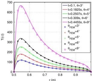
Fig. 7. Comparison of the temperature field.

mechanical behaviour up to an outer rotation angle of 3°, ensuring that the viscometer is completely elastic–plastic. Since the current time is involved in the thermal part of the solution, the rotation angle is prescribed on the outer cylinder in such a way that the plastic crown radius varies exponentially in time, using Eq.(24)connecting the curved arc length swept by the outer cylinder to the plastic crown radius.

For the thermomechanical calculation, an initial condition on the temperature respecting the analytical solution(54)is prescribed on each node of the mesh. The arbitrary parameter

µ

arising in the analytical solution(54)is set to 50 m−1_{. The} numerical problem now consists of 16 800 degrees of freedom as five unknowns are involved at each node of the mesh. Homogeneous Dirichlet boundary conditions are prescribed on the temperature degrees of freedom at the nodes of the inner and outer cylinders according to Eq.(52). The thermal conductivity

λ

, the density

ρ

and the heat capacity C are fixed to

λ =

600 W m−1_K−1

_{, ρ =}

_{2000 kg m}−3_{and C}

₌

_{150 J kg}−1_K−1_{, independently of the temperature. Since there is no} influence of the thermal part of the solution on its mechanical part, the latter part remains unchanged, seeFig. 6.

Comparisons between analytical and numerical temperatures are performed at times t

=

0

.

1, 0.1825, 0.2507, 0.309 and 0.4455 s, corresponding respectively to rotations of the outer cylinder of 3°, 4°, 5°, 6°and 9°, and are plotted in

Fig. 7. One can observe a very good agreement between these two solutions even for the last instant for which a very sharp peak of temperature close to the inner cylinder is apparent. This reflects the fact that the Couette viscometer thermomechanical problem for nonlinear solid-type behaviours represents a difficult numerical test involving large strains, heat generation through plastic dissipation and strong temperature gradients. The comparison just shown establishes the very good behaviour and the accuracy of the strongly coupled P1

+

/

P1 finite element in solid mechanics in a convincing manner.

6. Conclusion

In the present Part II, extensions of the classical Couette viscometer steady-state solution in fluid mechanics have been developed for solid-type nonlinear behaviours, first in the case of a purely quasi-static mechanical problem, and second in the case of a thermomechanical problem accounting for the generation of heat through plastic dissipation within the structure, in both small and large strains. These solutions permit to assess a new solid P1

+

/

P1 finite element developed in the framework of large strains with a temperature/velocity/pressure formulation.

In a first step, the quasi-static purely mechanical problem was addressed. The case of an elastic–plastic material obeying the von Mises criterion with isotropic hardening was considered. A solution was first found in the framework of small strains in Section2.1. The displacement field was found by integrating a function defined from the elastic–plastic constitutive law. It was also shown that the unloading of the Couette viscometer leads to a vanishing residual stress field. The extension to the large strain framework was performed using an additive decomposition of the Eulerian strain rate, and assuming that additional terms associated to the objective derivative of the stress were negligible. The solution developed in small strain was found to be unchanged with the sole replacement of the tangential displacement by the curved arc length swept.

In a second step, the Couette viscometer problem was addressed in thermo-elasto-plasticity in Section3, accounting for the generation of heat through plastic dissipation within the structure. The aim of the solution was to test the thermal part of the thermomechanical numerical solution computed with the P1

+

/

P1 finite element presented in Section4. With the assumptions of material parameters independent of temperature and negligible thermal dilation effects, a solution for the thermal part of the coupled problem applicable during the fully elastic–plastic regime of the loading was found using modified Bessel’s functions.

Section 4was devoted to the description of a temperature/velocity/pressure solid P1

+

/

P1 finite element in the framework of large strains, associated to an implicit (backward) Euler algorithm in time. This element is dedicated to the solutions of strongly coupled thermomechanical problems arising for example in welding applications.

The assessment of this finite element was subsequently performed in Section5. Both the mechanical and thermal parts of the numerical solution were compared to the analytical reference solutions developed. These comparisons showed a good agreement between both solutions, evidencing the good behaviour and the accuracy of the fully-coupled P1

+

/

P1 solid finite element developed.

Appendix. Extension of the solution of the Couette viscometer problem in elasto-plasticity to large strains

The extension discussed is done using the Eulerian setting, involving velocities instead of displacements. The definition of the strain given by(7)3is replaced by that of the Eulerian strain rate:

2Drθ

= ˙

γ =

d

v

_θ dr

−

v

θ r

=

d

˙

_l dr

−

˙

_l r (A.1)

where

v

_θdenotes the tangential component of the velocity, and l the curved arc length swept by a particle. Integration yields the expression of the ‘‘slip’’:

γ =

dl

dr

−

l

r (A.2)

where account has been taken of the fact that r remains constant in time for a given particle. Following the same approach as for small strains, the curved arc length l is expressed as a function of the shear stress

τ

through the constitutive law:

γ =

dl

dr

−

l

r

=

g

(τ(

r

))

(A.3)

where g is recalled to be a function defined from the inverse function of the constitutive law. Provided that the additional terms associated to the objective derivative in the hypoelastic law are neglected, the function g is still defined by Eqs.(20)

and(21)in the hypoelastic and hypoelastic–plastic zones respectively. Thus the curved arc length swept by a point located at the distance r from the origin is given by integration:

l

(

r

) =

r



r a g

(

r′

)

r′ dr ′

_.

(A.4) Thus, the solution developed for small strains remains unchanged provided that the tangential displacement u_θis replaced by the curved arc length swept l.

References

[1]D.N. Arnold, F. Brezzi, M. Fortin, A stable finite element for the Stokes equations, Calcolo 21 (1984) 337–344.

[2] T. Heuzé, Modélisation des couplages fluide/solide dans les procédés d’assemblage à haute température. Ph.D. Thesis, Université Pierre et Marie Curie, Paris, 2011 (in French).

[3] SYSWELD⃝R

, 2007. ESI Group. User’s Manual.

[4]R. Hill, The Mathematical Theory of Plasticity, Clarendon Press, Oxford, 1967.

[5]J. Salençon, De l’Élastoplasticité au Calcul à la Rupture, École Polytechnique, 2002 (in French).

[6]H.S. Carslaw, J.C. Jaeger, Conduction of Heat in Solids, second ed., Clarendon Press, Oxford, 1953.

[7]M. Abramowitz, I.A. Stegun, Handbook of Mathematical Functions: With Formulas, Graphs, and Mathematical Tables, Courier Dover Publications, 1965.

[8]Y.G. Duan, Y. Vincent, F. Boitout, J.B. Leblond, J.M. Bergheau, Prediction of welding residual distortions of large structures using a local/global approach, J. Mech. Sci. Technol. 21 (2007) 1700–1706.

[9]S. Souloumiac, F. Boitout, J.M. Bergheau, A new local–global approach for the modelling of welded steel component distortions, Math. Model. Weld Phenom. 6 (2002) 573–590.

[10]S.A. Tsirkas, P. Papanikos, K. Pericleous, N. Strusevich, F. Boitout, J.M. Bergheau, Evaluation of distortions in laser welded shipbuilding parts using a local–global finite element approach, Sci. Technol. Weld. Joining 8 (2003) 79–88.

[11]J.M. Bergheau, Y. Vincent, J.B. Leblond, J.F. Jullien, Viscoplastic behaviour of steels during welding, Sci. Technol. Weld. Joining 9 (2004) 323–330.

[12]J.B. Leblond, D. Pont, J. Devaux, D. Bru, J.M. Bergheau, Metallurgical and mechanical consequences of phase transformations in numerical simulations of welding processes, in: Lennart Karlsson (Ed.), Modeling in Welding. Hot Powder Forming and Casting, Vol. 42, ASM International, ISBN: 0-87170-616-4, 1997, pp. 61–89. (Chapter 4).

[13]L.E. Lindgren, Finite element modeling and simulation of welding. Part I: increased complexity, J. Thermal Stresses 24 (2001) 141–192.

[14]L.E. Lindgren, Finite element modeling and simulation of welding. Part II: improved material modeling, J. Thermal Stresses 24 (2001) 195–231.

[15]L.E. Lindgren, Finite element modeling and simulation of welding. Part III: efficiency and integration, J. Thermal Stresses 24 (2001) 305–334.

[16]L.E. Lindgren, Numerical modelling of welding, Comput. Methods Appl. Mech. Eng. 195 (2006) 6710–6736.

[17] É. Feulvarch, Y. Gooroochurn, F. Boitout, J.M. Bergheau, 3D modelling of thermofluid flow in Friction Stir Welding, in: S.A. David, T. DebRoy, J.C. Lippold, H.B. Smartt, J.M. Vitek (Eds.), Proc. 7th Int. Conf. on Trends in Welding Research, Pine Mountain, Georgia, USA, 16–20 May 2005, 2005, pp. 261–266. [18]É. Feulvarch, F. Boitout, J.M. Bergheau, Friction Stir Welding: modélisation de l’écoulement de la matière pendant la phase de soudage, Eur. J. Comput.

Mech. 16 (2007) 865–887 (in French).

[19]M. Bellet, O. Jaouen, I. Poitrault, An ALE-FEM approach to the thermomechanics of solidification processes with application to the prediction of pipe shrinkage, Internat. J. Numer. Methods Heat Fluid Flow 15 (2005) 120–142.