Multifractal analysis of the interstellar medium: first application to Hi-GAL observations

Multifractal Analysis of the Interstellar Medium. First application

to Hi-GAL Observations

Davide Elia,

1?

_{Francesco Strafella,}

2,3

_{Sami Dib,}

4,5

_{Nicola Schneider,}

6

_{Patrick Hennebelle,}

7,8,9

Stefano Pezzuto,

1

Sergio Molinari,

1

Eugenio Schisano,

1

Sarah E. Jaffa

10

Istituto di Astrofisica e Planetologia Spaziali, INAF, Via Fosso del Cavaliere 100, Roma, 00133, Italy 2_{Dipartimento di Matematica e Fisica ‘Ennio De Giorgi’, Università del Salento, CP 193, I-73100 Lecce, Italy} 3_{INFN Sezione di Lecce, CP 193, I-73100 Lecce, Italy}

4_{Niels Bohr International Academy, Niels Bohr Institute, Blegdamsvej 17, DK-2100, Copenhagen, Denmark} 5_{Max-Planck Institute für Astronomie, Königstuhl 17, 69117, Heidelberg, Germany}

6_{I. Physik. Institut, University of Cologne, D-50937 Cologne, Germany} 7_{IRFU, CEA, Université Paris-Saclay, 91191 Gif-sur-Yvette, France}

8_{Université Paris Diderot, AIM, Sorbonne Paris Cité, CEA, CNRS, 91191 Gif-sur-Yvette, France} 9_{LERMA (UMR CNRS 8112), Ecole Normale Supérieure, 75231 Paris Cedex, France}

10_{School of Physics and Astronomy, Cardiff University, Cardiff CF24 3AA, Wales, UK 0000-0002-6711-6345}

Accepted XXX. Received YYY; in original form ZZZ

ABSTRACT

The multifractal geometry remains an under-exploited approach to describe and quantify the large-scale structure of interstellar clouds. In this paper, the typical tools of multifractal analysis are applied to Herschel far-infrared (70-500 µm) dust continuum maps, which represent an ideal case of study. This dust component is a relatively optically thin tracer at these wavelengths and the size in pixel of the maps is well suitable for this statistical analysis. We investigate the so-called multifractal spectrum and generalised fractal dimension of six Hi-GAL regions in the third Galactic quadrant. We measure systematic variations of the spectrum at increasing wavelength, which generally correspond to an increasing complexity of the image, and we observe peculiar behaviours of the investigated fields, strictly related to the presence of high-emission regions, which in turn are connected to star formation activity. The same analysis is applied to synthetic column density maps, generated from numerical turbulent molecular cloud models and from fractal Brownian motion (fBm), allowing for the confrontation of the observations with models with well controlled physical parameters. This comparison shows that, in terms of multifractal descriptors of the structure, fBm images exhibit a very different, quite unrealistic behaviour when compared with Hi-GAL observations, whereas the numerical simulations appear in some cases (depending on the specific model) more similar to the observations. Finally, the link between mono-fractal parameters (commonly found in the literature) and multifractal indicators is investigated: the former appear to be only partially connected with the latter, with the multifractal analysis offering a more extended and complete characterization of the cloud structure.

Key words: ISM: clouds – ISM: structure – Infrared: ISM – stars: formation – methods: statistical – techniques: image processing

1 INTRODUCTION

The complex morphology of Galactic interstellar clouds generally eludes a description simply based on the typical shapes of Euclidean geometry (e.g., Scalo 1990; Elmegreen & Falgarone 1996; Pfen-niger 1996). The mostly self-similar appearance of the interstellar medium (ISM), especially at scales L & 1 pc is generally thought

? _{E-mail: [email protected]}

to be the result of turbulence (Elmegreen 1995; Elmegreen & Scalo 2004; Dib & Burkert 2005; Krumholz 2014), because of the intrin-sic self-similarity of this phenomenon, triggered by the very high value of the Reynolds number in these environments. The fractal ge-ometry is largely invoked to provide a quantitative characterization of the ISM morphology, as it can be deduced from far-infrared (FIR) or sub-millimetre maps, through fractal descriptors (Stutzki et al. 1998; Bensch et al. 2001; Schneider et al. 2011; Sun et al. 2018; Elia et al. 2014, hereafter Paper I) and comparing these quantities with

theoretical expectations has two important advantages. On the one hand, a comparison between models and observations gives indica-tions about the kind of turbulence that is prevalent in the observed cloud and, on the other hand, the obtained fractal parameters can be used as further constraints for future simulations. In this respect, fractal or, in a broad sense, statistical analysis techniques are applied also to numerical simulations of turbulent clouds, to make possi-ble a comparison between model and ISM morphological proper-ties. Three-dimensional magneto-hydrodynamic simulations have been characterised in terms of probability density function, struc-ture function and power spectrum (Kowal et al. 2007; Kritsuk et al. 2007), fractal dimension (Federrath et al. 2009), or dendrograms (Burkhart et al. 2013).

It should also be emphasised that natural fractal structures, such as ISM, are self-similar only in a statistical sense (stochastic

fractals) and show complexity only over a finite range of scales.

Identifying such a range, which should correspond to the scales actually involved by the turbulent energy cascade, can give impor-tant information on the injection and dissipation scale of turbulence (see Paper I, and references therein). Interestingly, the latter is ex-pected to correspond to the characteristic size of gravity-dominated structures (filaments and cores) relevant for star formation, as high-lighted, e.g., by Falgarone et al. (2004) and Schneider et al. (2011) (for more recent analysis of the turbulence-regulated star formation, see also Burkhart et al. 2017; Mocz et al. 2017).

This (mono-)fractal approach, however, still underlies a certain degree of degeneracy: as said above, a large number of natural ob-jects exhibit properties of self-similarity, but can not be described as perfect fractals, especially because such a description is based on a sole parameter, namely the fractal dimension. In contrast,

Multi-fractal geometryprovides a more suited mathematical framework

for detecting and identifying complex local structure, and for de-scribing local singularities. It is invoked in the fields of economy, medicine, hydrography, environmental sciences, and physics (e.g. in studying turbulent flows). In astrophysics, it has been used, for example, in the study of the distribution of galaxies (Mandelbrot 1989; Borgani et al. 1993; Pan & Coles 2000; de La Fuente Mar-cos & de La Fuente MarMar-cos 2006), gamma-ray burst time series (Meredith et al. 1995), and solar activity (Wu et al. 2015; Cadavid et al. 2016; Maruyama et al. 2017).

The first application of the multifractal approach to charac-terize the ISM structure was carried out by Chappell & Scalo (2001), who analyzed 13 IRAS maps (at 60 and 100 µm) taken from Chamaeleon-Musca, R Corona Australis and Scorpius-Ophiucus star forming regions, all located at distance d < 160 pc from the Sun, but spanning a relatively wide range of different conditions of star formation. A multifractal behaviour of the investigated clouds was revealed over the range 0.4-4 pc, and a possible relation with underlying turbulent cascades and hierarchical structure was found. While the multifractal properties of a cloud can be directly related to its geometry, a direct relation with the properties of the star for-mation is not found by these authors; this link has been established indirectly for the first time by Tassis (2007) using global param-eters of external galaxies. Finally, Khalil et al. (2006) studied the multifractal structure of Galactic atomic hydrogen through wavelet transform techniques, discussing arm vs inter-arm differences.

As already pointed out in Paper I, the advent of Herschel (Pil-bratt et al. 2010) offered an extraordinary chance for studying the morphology of the cold Galactic ISM, thanks to the combination of several favourable conditions and features: i) the spectral coverage of Herschel photometric surveys (70 − 500 µm) encompasses the peak of the continuum emission of cold dust (T ≤ 50 K), with

the dust getting optically thinner at increasing wavelengths, which helps revealing the structure of dense clouds with unprecedented accuracy; ii) the angular resolution of Herschel photometric obser-vations (600

−3600) is better or comparable with that of the most recent CO surveys of the ISM (e.g., Jackson et al. 2006; Burton et al. 2013; Schuller et al. 2017), and their dynamic range is so large (more than two orders of magnitude, e.g., Molinari et al. 2016) that the obtained 2-D picture of the ISM structure generally turns out to be highly detailed and reliable; iii) large Herschel photometric surveys produced a huge amount of data, corresponding to a wide variety of Galactic locations, physical conditions, and star forma-tion modes to be compared; iv) thanks to good angular resoluforma-tion and excellent mapping capabilities, single Herschel maps represent highly suitable data sets for pixel statistical analysis, namely tech-niques aimed at deriving fractal properties of maps starting from intensity values in single pixels. This improvement can be appreci-ated, for instance, by comparing how much the size in pixels of the analysed maps increased from the pioneering work of, e.g., Stutzki et al. (1998) (several tens or a few hundred pixels) to that of Paper I (up to a few thousands of pixels).

Despite this potential, the promising approach of Chappell & Scalo (2001) for describing the structure of the ISM through mul-tifractal parameters has not been yet applied to Herschel maps. With this paper we intend to fill this gap. Furthermore, choosing the same fields already analysed through mono-fractal descriptors in Paper I, we explore possible relations between mono- and multifrac-tal parameters for any investigated field. Finally, analysing with the same techniques also column density maps obtained from numer-ical simulations of insterstellar turbulence, we search for possible recipes connecting the quantitative description provided by multi-fractal tools and the underlying physics of the analysed regions.

The paper is organized as follows: in Section 2 the analysed maps, both observational and synthetic, are presented. In Section 3 basics of multifractal geometry are introduced, together with a de-scription of the tools used in the rest of the paper. In Section 4 the results of the multifractal analysis of the aforementioned data sets are reported and discussed by means of specific diagnostics, while our conclusions are given in Section 5. Additional details and discussion of the method are reported in the Appendices A, B, and C.

2 ANALYSED FIELDS 2.1 Hi-GAL maps

The observational sets chosen for this analysis are six 1.5◦

×1.5◦ fields extracted from the Hi-GAL programme (Molinari et al. 2010), the photometric survey of the entire Galactic plane carried out at the 70, 160, 250, 350, and 500 µm wavelengths with the two cameras PACS (Poglitsch et al. 2010) and SPIRE (Griffin et al. 2010). The original ∼ 2.2◦_×2.2◦_{Hi-GAL tiles obtained in the five}

aforementioned bands have a nominal resolution1 of 5.600_{, 11.3}00_,

17.600_{, 23.9}00_{, and 35.1}00_{, and a pixel size of 3.2}00_{, 4.5}00_{, 6}00_{, 8}00_,

and 11.500_{, respectively (Molinari et al. 2016).}

The fields were chosen in the third Galactic quadrant (Elia et al. 2013): the central four, designated as `217, `220, `222, `224

1 _{Actually, due to the PACS data co-adding on-board Herschel, the resulting} point-spread functions are elongated along the scan direction, with a mea-sured size of 5.800_×12.100_{at 70 µm, and 11.4}00_×13.400_{at 160 µm, respectively} (Lutz 2012).

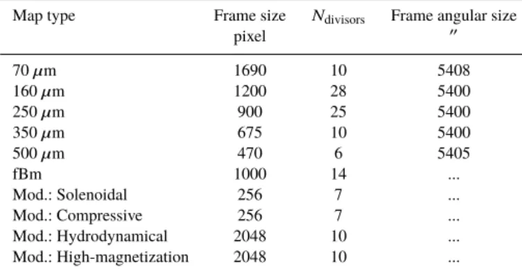
Table 1.Geometric properties of analysed frames.

Map type Frame size Ndivisors Frame angular size

pixel 00 70 µm 1690 10 5408 160 µm 1200 28 5400 250 µm 900 25 5400 350 µm 675 10 5400 500 µm 470 6 5405 fBm 1000 14 ... Mod.: Solenoidal 256 7 ... Mod.: Compressive 256 7 ... Mod.: Hydrodynamical 2048 10 ... Mod.: High-magnetization 2048 10 ...

(from the original names of Hi-GAL the tiles they were extracted from), respectively, are already described (including data reduction and map making details) in Elia et al. (2013) and in Paper I. These fields were selected based on the following considerations:

(i) Ideally, each selected field should contain emission from a single Galactic component, i.e. from dust distributed within a lim-ited range of heliocentric distances. In this portion of the Galactic plane, NANTEN data (Onishi et al. 2005; Elia et al. 2013) show a simple structure of the velocity field (Paper I, their Figure 1), so that each of the chosen Hi-GAL fields can be associated with a single predominant velocity component, i.e. a single coherent cloud.

(ii) The clipping of original tiles must be performed on the area observed by both PACS and SPIRE, choosing the same box for all the five bands, in order to analyse the same area of the sky at all wavelengths, in the limit of pixelation.

(iii) The clipped maps are chosen to be square-shaped and must be as large as possible, in order to increase the statistical relevance of the results and expand the range of spatial scales that are probed. In addition to these requirements, for this work we also impose that (iv) The size of the analysed maps must be a number of pixels characterised by a large enough number of integer factors, for the reasons that will be explained in Section 3.3.

About cropping the maps, it is difficult to find a common angu-lar size, for all the five bands, which contextually corresponds to sizes (in pixels) satisfying the aforementioned property. For this reason we slightly adjusted the number of pixels composing the maps at each band, finding a final set of frame sizes in pixels ap-proximately corresponding to 1.5◦_{(depending on the wavelength,}

see Table 1). As a consequence, the maps analysed in this work turn out to be slightly smaller than those for which the fractal dimension was derived in Paper I, making it necessary to re-compute it (see Appendix C) in view of a comparison with multi-fractal properties (Section 4.3).

In Table 1 we report for each band the size of the maps in pixels, and the corresponding number of factors2and angular scale in arcseconds.

Furthermore, we include the two Hi-GAL tiles `215 and `226 that extend the sample to the West and to the East, respectively. In total, we have six tiles in five bands plus column density maps, i.e.

2 _{For example, at 350 µm the chosen map size is 675 × 675 pixels. Except} for 1 and itself, the side 675 has the following integer divisors: 3, 5, 9, 15, 25, 27, 45, 75, 135, 225, which therefore allow to perfectly cover the map with 10 possible box grids, and so on.

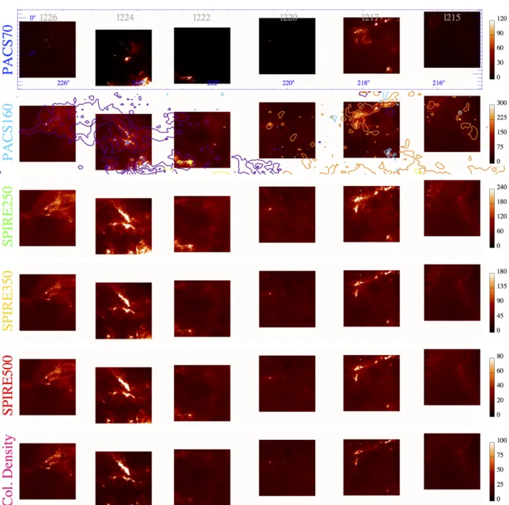
a total of 36 maps analysed in this work. All maps are displayed in Figure 1.

In Elia et al. (2013) an analysis of the gas velocity field, as de-rived from NANTEN CO(1-0) spectral line observations, was car-ried out for the four central tiles. It highlighted a prominence of emis-sion from a closer component (at distances around hdiI= 1.1 kpc)

for the two Eastern tiles `224 and `222, and from a farther compo-nent (around hdiII= 2.2 kpc) for the two Western ones, `220 and

`217. These two components are also spatially segregated, since their reciprocal contamination degree is very low in the NANTEN data. Moreover, the contamination from two further and fainter ve-locity components (hdiIII= 3.3 kpc, hdiIV= 5.8 kpc), is negligible

in turn, even more after appropriate map cropping (see Figure 1). In the four central panels of the second row in Figure 1 the low degree of contamination for the four corresponding Hi-GAL fields can be appreciated. This made it possible, in Paper I, to associate each tile to only one of the two main velocity components of the region. In this paper, with the additional `215 and `226 tiles, we extend the basic analysis of the velocity field to these tiles. Looking at CO intensity contours obtained separately for each of the four aforementioned Galactic components, and overplotted on Hi-GAL 160 µm maps (Figure 1, second row, the leftmost and rightmost tile, respectively), one can see how the region in `226 is dominated by component I, whereas the one in `215 is dominated by compo-nent II, so that, in conclusion, we can associate the three Eastern tiles to component I, and the three Western ones to component II, respectively.

2.2 Turbulent ISM simulations

We compare the observational data to the density structures found in 3-dimensional numerical simulations provided by the STAR-FORMAT project3, a database containing results of high-resolution numerical simulations computed to study the formation, evolution and collapse of molecular clouds4_{. Among the available projects,}

we chose the two we describe in the following. The “Solenoidal vs. compressive turbulence forcing” project was carried out by Feder-rath et al. (2008) in order to investigate differences between models of these two limiting regimes characterised by different mechanisms of kinetic energy injection. Simulations were performed using the FLASH3 code (Fryxell et al. 2000; Dubey et al. 2008), solving hydrodynamic equations on 10243cubes, assuming an isothermal gas (self-gravity is not included). Snapshots of the cube are avail-able, for both scenarios, at different time steps, calibrated on the timescale parameter T = L/(2csM), where L is the size of the

computational domain, cs the sound speed and M the rms Mach

number. To explore possible structure variations at two different epochs, we considered the second and the second last available time steps, namely for t1= 3T and t2= 9T .

The used data sets consist of the column density maps obtained projecting the density cube along one of the three axes, say x (then, in this convention, in the yz plane), and rebinned onto a 2562_pixel

grid. Moreover, to investigate possible projection effects, also the projection in the xy plane of the cube at the time t1has been used.

3 _{starformat.obspm.fr}

4 _{Among other interesting resources for downloading numerical simulations} of the ISM, we advide also Galactica (http://www.galactica-simulations.eu), CATS (http://mhdturbulence.com), and the John’s Hopkins Turbulence Databases (http://turbulence.pha.jhu.edu), not used for this work.

Figure 1.Each row shows the six Hi-GAL fields investigated in this paper. The instrument/band combination is specified in each row, adopting the color convention that is used throughout the rest of the paper, namely blue: 70 µm, cyan: 160 µm, green: 250 µm, yellow: 350 µm, red: 500 µm, magenta: column density. The color scales are linear; we preferred this choice with respect to the logarithmic scale to show the actual dynamics of the maps processed in this paper. The units are MJy sr−1_{for the PACS and SPIRE maps, and 10}20_cm−2_{for the column density ones. The tile names and Galactic coordinate grid are} displayed in the row of 70 µm images (longitude on the horizontal axis and latitude on the vertical axis). Notice that the frame displacement is a real effect due to the choice of square area cut from each original tile. The CO(1-0) contour levels of Elia et al. (2013) are overplotted on the row of 160 µm images. The contours start from 5 K km s−1_{and are in steps of 15 K km s}−1_{. Velocity components I, II, III, and IV (see text) are represented with purple, orange, yellow,} and cyan contours, respectively.

In conclusion, exploring two scenarios (solenoidal and compres-sive), two epochs and an alternative projection direction for the first epoch, six different maps were included in our analysis (Figure 2, top two rows). Images corresponding to the two different scenarios appear quite different, being the compressive forcing maps charac-terised by a sharper contrast between very bright and extended void regions. Differences in structure have been already highlighted and quantified by Federrath et al. (2008, 2009, 2010) through

proba-bility density function and power spectrum/∆-variance analysis. In Paper I a generally better consistency in terms of power spectrum slope/fractal dimension has been found between the four central Hi-GAL fields analysed in this paper and the solenoidal case rather than the compressive one.

The second project selected in the STARFORMAT data base is “Molecular cloud evolution with decaying turbulence” (Dib et al. 2010; Soler et al. 2013), which aims at describing a self-gravitating

Figure 2. Column density maps obtained by projecting 3-dimensional simulated density fields selected in the STARFORMAT archive. The rows, from top to bottom, correspond to four different scenarios, namely “solenoidal forcing”, “compressive forcing”, “quasi-hydrodynamical”, and “high-magnetization”, respectively (see text). The images in the upper two rows are composed by 256 × 256 pixels, while those in the lower two rows are composed by 2048 × 2048 pixels, see Table 1. In each column a different combination of epoch and projection direction is displayed: the assignment of yz and xy plane denominations follows the notation used in STARFOR-MAT, used here only to indicate that the two planes are orthogonal. With t1 and t2we do not indicate, in general, the same time for all the four scenarios, but only two different epochs such that t1< t2; they coincide for the first and the second scenario only. Further details of the simulations are reported in the text. Maps are represented here by arbitrarily normalising their values by the map average hI i, and rendered through a logarithmic scale, choosing an image saturation level of log10(10hI i), to better appreciate the low-density fluctuations.

cloud with decaying turbulence in presence of a magnetic field. We considered two limiting scenarios with a weak and a strong mean magnetic field (B < 4 µG and B > 20 µG, respectively), called “quasi-hydrodynamical” and “high-magnetization” case, respec-tively. Simulations were performed through the RAMSES-MHD code (Teyssier 2002; Fromang et al. 2006) and produced cubes with an effective resolution of 20483elements reproducing a 4 pc-wide region hosting a cloud with a mass of ∼ 2000 M. Two snapshots are

available, in correspondence of t1 = 0.49 Myr and t2 = 1.16 Myr

for the former scenario, and t1 = 0.61 Myr and t2 = 1.15 Myr for

the latter, respectively. Also in this case, the projection of the density field in the yz plane has been taken at these two epochs, together with the projection in the xy plane at the earliest of the two epochs. The selected fields are shown in the last two rows of Figure 2.

2.3 Fractional Brownian motionimages

The fractional Brownian motion images (fBm, Peitgen & Saupe 1988) are often used as a surrogate of ISM maps thanks to their visual similarity with cloud features (Stutzki et al. 1998; Bensch et al. 2001; Miville-Deschênes et al. 2003). Their analytic properties are fully described in Stutzki et al. (1998) and recently resumed in Paper I, to wich we refer the reader for more details. Here, we simply remind their basic properties: i) their radially averaged power spectrum exhibits a power-law behaviour, and ii) the distribution of the phases of their Fourier transform is completely random. These images are fractal, with a precise analytic relation between their (mono-)fractal dimension D (see Section 3) and the power-spectrum power-law exponent β:

D= 4 −β

2, (1)

which is valid for a signal defined over a two-dimensional space (Stutzki et al. 1998).

In this paper, we use these images as a reference, since they can be obtained with preconditioned statistical properties. In particular we generated a set of 1000×1000 pixels fBm images by exploring a two-dimensional parameter space, i.e. varying both the β exponent (then the global fractal dimension) from 2 to 4 in steps of 0.4 (cf. Paper I), and the distribution of the phases, initializing the random number generator with three different “seeds”, called hereafter re-alization A, B, and C. A given phase distribution determines the global appearance of the image as a “cloud”, while increasing β produces a gradual smoothing of the image, due to the transfer of power from high to low spatial frequencies, as it can be seen in Figure A1 (Appendix A).

3 MULTIFRACTAL ANALYSIS

As pointed out in Section 1, the multifractal analysis represents an extension of the fractal theory, aimed at enhancing and enriching the characterization of a non-deterministic (i.e. natural) fractal. It is closely related to the concept of generalized fractal dimension.

3.1 Generalized fractal dimension

The fractal dimension, introduced by Mandelbrot (1967), is one of the fundamental concepts in fractal analysis. It expresses the degree of complexity of a self-similar object, and in particular its ability to fill the hosting space. Importantly, it is not an integer num-ber, exceeding the Euclidean dimension of the set (e.g., the fractal dimension of a fractal line is larger than 1, the one of a fractal surface is larger than 2, etc.). In this respect, the fractal dimen-sion represents a meaningful indicator for quantifying the structure of complex, nested, convoluted structures which depart from the smooth appearance of Euclidean shapes. Nevertheless, the need of going beyond a single descriptor, leads to the formulation of the multifractal geometry, based on the concept of fractal generalized

dimension.

The definition of a set of dimensions of order q ∈ R is due to Hentschel & Procaccia (1983), who introduced this concept to improve the characterization of chaotic attractors of dynamical sys-tems. A single parameter constitutes an incomplete characterization of such sets, which are not perfectly self-similar by construction like, instead, the deterministic examples (such as the well-known Can-tor set or the Koch curve). The generalized dimensions, therefore,

represent an attempt to address in a more general way the charac-terization of the so-called “strange sets”.

Among various formulations of the generalized dimensions, here we briefly report the one based on the box-counting approach (cf. Hentschel & Procaccia 1983): let us start considering a set constituted by points (as, for example, black pixels in an image with a white background), in this context generally named measure, and cover it with boxes of size ε. Let us define the probability of points contained in the i-th box as Pi = Ni/N, where Ni is the number of

points in the i-th box, out of a total number of points N. The q-th generalized dimension Dqis defined as

Dq = lim ε→0 1 q −1 log ÍiPiq log ε . (2)

Defining the partition function of the q-th order as Zq(ε) =

Õ

i

P_iq, (3)

the definition in Equation 2 becomes Dq = lim ε→0 1 q −1 log Zq(ε) log ε . (4)

Notice that the case q = 0 recovers the classic expression of the box counting mono-fractal dimension D (e.g., Falconer 2003). An interesting case is D1(also called information dimension), obtained

from Equation 2 in the limit q → 1. By construction, all the Dq

dimensions of a deterministic pure fractal will coincide with D, while a multifractal is an object whose generalized dimensions are quite different. The Dq values monotonically decrease with

increasing q (Hentschel & Procaccia 1983), and the lower and upper limiting dimensions, named D−∞and D_+∞, respectively, are related

to the regions of the set in which the measure is “most diluted” and “most concentrated”, respectively.

In general, the partition function of multifractal sets scales as

Zq(ε) ∝ ετq, (5)

(e.g., Arneodo et al. 1995), with τqnamed correlation exponent of

order q. The relationship between τqand q is expressed by

τq= q h(q) − E , (6)

where E indicates the Euclidean dimension of the volume hosting the fractal, named support of the measure (e.g., Gu & Zhou 2006). For a monofractal, the h(q) coefficient is constant (and called Hurst

exponent) so that the τqvs q relation is linear, whereas in the more

general case of a multifractal h(q) (in such case called generalized

Hurst exponent) varies as a function of q.

Finally, combining Equations 4 and 5 one finds

τq= (q − 1)Dq (7)

(Halsey et al. 1986). As a particular case of this equation, it is found that D0= −τ0.

At this point, some caveats about the interpretation of the introduced quantities and their application to astronomical maps (or to grey-scale images in general) need to be pointed out. Indeed, all the above definitions and considerations are strictly valid for a measure composed by discrete points, when a coverage of the support of the measure is performed. In our case, the measure is a 3-D surface having values different from zero at any point of its support, which is a m × n pixels raster. The probability Pi is the

sum of the brightnesses of all pixels falling inside the i-th box, normalized by the integral over the entire map. With this approach, it can be seen that, for q = 0, Equation 2 does not return the true

fractal dimension of the investigated image, but rather the Euclidean dimension of the support of the measure, in other words one finds D₀= 2 for all images.

3.2 Multifractal spectrum

A tool typically used for the multifractal analysis is the so-called

sin-gularity spectrum, or multifractal spectrum (MFS), first introduced

by Halsey et al. (1986).

Let us consider a measure (here our Hi-GAL maps) embedded in a support and cover it with boxes of size ε as already discussed in Section 3.1. If the measure is a multifractal, the probability Piscales

with ε as a power law with exponent αi(also known as singularity

strength), as a function of the position: Pi(ε) ∝ εαi. Given the

fractal dimension f (α) of the subset of boxes having singularity strength in the range (α, α + dα), the MFS is just the curve of f (α) vs α. It represents the contributions to the geometry provided by interwoven sets with different singularity strengths.

The relation between the MFS and the generalized dimensions is expressed by the Legendre’s transform:

α(q) =dτq

dq (8)

f (α(q)) = qα(q) − τq (9)

(Halsey et al. 1986). In this sense, the MFS can be calculated im-mediately after deriving the (q, Dq) pairs.

From these relations the following properties of the f (α) curve are derived:

df

dα =q (10)

d2f

dα2 < 0 . (11)

Therefore, the MFS is concave for any measure, with a single max-imum at q = 0 (then f (α(0)) = D0 for a measure constituted by

points5), and with infinite slope at q = ±∞.

The MFS gives information about the relative importance of various fractal exponents present in the map, and in particular its width indicates the range in which such exponents lie. The part cor-responding to values q > 0 characterises the scaling properties of overdense regions because it magnifies the effect of large numbers, while for q < 0 the behaviour of low-density subsets is charac-terised. This generally results in an asymmetrical shape of the MFS with respect to its peak position (q = 0).

3.3 Practical derivation of multifractal parameters

For the purpose of this paper we derive the values of τqand Dqfor

each map through the partition function, as described in Section 3.1. The analysed sets are constituted by a discrete number of pixels, thus we partition the data sets in boxes with integer size ε. In this respect, it is preferable to deal with image sizes that have a large number of integer divisors (see Section 2.1) enough to ensure a sufficiently

5 _{As already pointed out in Section 3.1, here wee analyse greyscale images.} In this case, f (α(0)) coincides with the Euclidean dimension of the support of the measure, namely 2, as it can be seen, in the following, from Equation 14 combined with Equation 12.

0.5 1.0 1.5 2.0 2.5 3.0 Log[ε] -60 -40 -20 0 20 40 60 Log[Z q ( ε)] -10 -9 -8 -7 -6 -5 -4 -3 -2 -1 0 1 2 3 4 5 6 7 8 9 10 q = -10 -5 0 5 10 15 20 q -20 -10 0 10 20 30 τq -10 -5 0 5 10 15 20 q 1.95 2.00 2.05 2.10 2.15 2.20 2.25 Dq

Figure 3.Example of derivation of the generalised fractal dimensions for a test 1000 × 1000-pixel fBm image (see Section 2.3), in this case the one of type “C” and β = 2.4 shown in Figure A1. Left: logarithm of the partition functions Zq(ε) vs the logarithm of the integer scales ε between 1 and 500 pixels for each integer value of the parameter q between -10 and 10 (in this range, different shades of blue, from the darkest to the lightest, respectively, are used for each different q). The linear fit is shown as a dashed line of the same colour of the corresponding Zqfunction (cf. Equation 5). The functions for orders q > 10 and non-integer orders in the range −2 < q < 2, although computed, are not shown here for the sake of clarity. Middle: scaling exponents τqof the partition function, obtained through the linear fit shown in the left panel as a function of q. To highlight the different slopes at negative and positive orders, the linear fit of the τqvs q in the two the regions q < −3 and q > 3, is shown by means of two grey lines. Right: generalised fractal dimension set, derived through Equation 7, as a function of q, except for the case q = 1, not contemplated by Equation 7.

2.0 2.1 2.2 2.3 2.4 2.5 α -0.5 0.0 0.5 1.0 1.5 2.0 f( α ) q > 0 q < 0 2.0 2.1 2.2 2.3 2.4 2.5 α -0.5 0.0 0.5 1.0 1.5 2.0 f(α)

Figure 4. Left: MFS of the same fBm reference image used to build Figure 3, obtained through Equations 8 and 9, exploring the range of orders −10 ≤ q ≤20, in steps of ∆q = 1 (but ∆q = 0.2 in −2 ≤ q ≤ 2). The error bars are displayed as grey crosses for each point, to give an idea of the typical uncertainties affecting the MFS estimation. Right: The same as in the left panel, but computed through Equations 13 and 14.

large range of investigated spatial scales, i.e. points to sample the behavior of the right-hand side of Equation 4.

In Figure 3 we show a derivation of these quantities for a fBm test image shown in Figure A1, third-row and third-column panel, corresponding to realization “C” and power spectrum slope 2.4. For this example, as well as for all maps analysed in this paper, the probed range of orders q is −10 ≤ q ≤ 20, in steps of ∆q = 1, except for the interval −2 ≤ q ≤ 2, which is explored in steps of ∆q = 0.2 to better sample a critical region for multifractal descriptors (slope change for τq, inflection point of Dq, and peak of the MFS around

q= 0, see below).

The Zq(ε) function (left panel) shows the expected power-law

behaviour, from which the τq scaling fits can be derived through

a linear regression procedure (Equation 5). The quality of such fit determines in turn the extent of the error bar on τq. The τq vs q

curve (middle panel) does not present a single linear behaviour, but a typically multifractal behaviour with two different slopes for the two q < 0 and q > 0 regimes, and a non-linear behaviour in the transition zone (cf., e.g., Movahed et al. 2011; Xie et al. 2015). Similarly, the obtained Dqvs q curve (right panel) is far from being

constant (cf., e.g., Halsey et al. 1986; Meneveau & Sreenivasan 1987), confirming that the analysed image presents a multifractal rather than a simple mono-fractal character.

Once τqand Dqare obtained, the MFS can be derived through

Equations 8 and 9. Another linear fit is requested in this case, introducing a larger uncertainty on both α and f (α). An alterna-tive method for calculating directly the MFS was developed by Chhabra & Jensen (1989) and applied by Chappell & Scalo (2001) for estimating the MFS of IRAS maps. Defining the coarse-grained moments µi(q, ε) of the original image as

µi(q, ε) =

Pq_i(ε) Í

iPiq(ε)

, (12)

α and f (α) are implicitly defined with respect to the q parameter through α(q) = lim ε→0 Í iµi(q, ε) log Pi(ε) log ε (13) f (q)= lim ε→0 Í iµi(q, ε) log µi(q, ε) log ε . (14)

In practice, in the case of an ideal multifractal, the quantities whose limits are calculated in the right sides of the equations above show a linear behavior, since the limits can be extrapolated from a linear fit. Consequently, the uncertainties associated to α(q) and f (α(q)) mainly depend on the quality of such fit. Again, we reaffirm, also

for this approach, the need of analysing images with sizes divisible by a large number of integer factors.

In Figure 4, we compare the MFS obtained for the same fBm image using the two methods. The spectra look practically identical, with differences smaller than 1% in all cases, while the error bars, which are generally much larger for q < 0, are comparable for α but larger for the first metod for f . For this reason, in the following we will show MFSs obtained through the Chhabra & Jensen (1989) method (Equations 13 and 14), keeping the first one as a reference for checking the correctness of the results.

4 RESULTS OF MULTIFRACTAL ANALYSIS

The multifractal behaviour of the analysed maps can be examined by means of both the generalised dimension formalism (Dqvs q)

or the MFS one ( f (α) vs α). We start from the latter, which allows us to better highlight some peculiarities in our map sample with respect to the scaling implied by Equation 3.

4.1 Qualitative analysis of MFS

In Figure 5 the MFS of each Hi-GAL tile at each band are shown, while in Table 2 a number of salient parameters of the MFS, some of which introduced in the following Section 4.2, are listed6_{. It is}

possible to make some initial and general considerations about the overall appearance of the spectra:

• In general, the MFSs present a typical single-humped shape with a maximum at f0 = 2 (i.e. the Euclidean dimension of the

support, as explained previously), but a strong negative skewness. • In several cases, at high q (i.e. at the left end of the MFS) a cusp-like turnback of α(q) appears in the spectrum (the most evident case being found for the 70 µm map of `224, but other cases are well recognisable in the plots of Figure 5). Such a fea-ture (cf. Lou et al. 2015) can be considered i) as a computational artefact, due to the presence of spatial heterogeneity of brightness in the image which leads to disproportionate contribution of boxes containing rare extremely intense pixels during averaging over the whole area, and ii) as a real effect related to intrinsic statistical prop-erties of the analysed image departing from those of a multifractally distributed measure. Wolf (1989), indeed, demonstrated that this feature appears in correspondence of a breakdown in the scaling law expressed by Equation 5 at orders higher than a critical value q+_c (see also, e.g., Abry et al. 2004). Most likely, the appearance of such a cusp is produced by a combination of these two effects in im-ages presenting a wide dynamic range between the diffuse emission and few very bright compact sources. In Table 2 a possible presence of a cusp in the MFS is reported by listing the possible value of q+

c.

The maps affected by this problem will suffer of some limitations throughout the analysis carried out in this paper, since the part of the spectrum corresponding to q > qc+(missing data in Table 2)

will not be taken into account.

• In most cases, the right portion of the MFS for the 70 µm maps turns out to be collapsed to a very short branch close to the peak, while the left portion (in correspondence of positive q values) appears extremely elongated. In general, a MFS shows a long left tail when the signal has a multifractal structure which is

6 _{Notice that hereafter, for the MFS coordinates corresponding to a given} order Q we use the simplified notation αQand fQin place of α(q = Q) and f (q = Q), respectively.

insensitive to the local fluctuations with small amplitudes, and a shrunk right tail in presence of a small scale noise-like background (e.g., Drożdż & Oświe¸cimka 2015). This is the typical case of Hi-GAL 70 µm maps in this portion of the Galaxy generally showing rare and isolated bright spots, corresponding to episodes of star formation, and a very faint background emission often surmounted by the instrumental noise. This fact, together with the frequent occurrence, for the 70 µm maps, of the aforementioned cusps in the MFS, makes the maps at this wavelength a peculiar case in our multi-fractal analysis, showing in general a departure from a fractal behaviour.

• For each tile, the MFSs of the SPIRE images show a relatively similar behaviour, but not identical. The positions of the extreme points can differ, even significantly, from band to band depend-ing on the tile, the strongest differences bedepend-ing found in the tiles containing the brightest features, i.e. `217, `224, and `226. Such overall similarities and fine-scale differences will be highlighted in the following more quantitative analysis.

• The 160 µm maps show a behaviour of the MFS width which is intermediate between the 70 µm and the SPIRE ones, being the q < 0 tail less pronounced than for the SPIRE maps, but not collapsed as generally found for the 70 µm ones.

• Finally, the column density maps, which could be expected to have a behaviour similar to the SPIRE ones, actually differ signif-icantly from them in some cases, especially for the tiles `217 and `224.

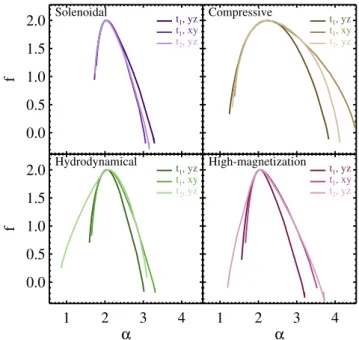
The MFS was derived also for all the simulated column den-sity fields described in Section 2.2 and shown in Figure 2. All the computed MFSs are plotted in Figure 6, each panel corresponding to a different model. In the following, we summarize some results of the comparison among the different models and their projections and epochs, and with the Hi-GAL observations

First, the MFSs of the simulations look quite different, in gen-eral, from those of the Hi-GAL maps. Particularly on the right side of the curve, for the simulations the largest value of α, correspond-ing to the most negative explored q, is larger than the one of the observations (a more quantitative description of this aspect will be given in Section 4.2). Notice also that for some spectra cusps like those described above, but located at the opposite extreme, appear. In some cases, the cusp can not be noticed in the figure because the turnaround point is found close to q = −10 and the following points are very close to those of the “regular” part of the MFS. Anyway, in Table 3 we account for the possible occurrence of such an effect for qsmaller than a critical q−_c, together with possible occurrences of cusps in the q > 0 portion of the spectrum as well, and with other relevant parameters of the MFSs, similarly to Table 2.

Second, remarkable differences are found among the models: the “compressive forcing” case shows much wider spectra with ex-tended right tails, produced by the presence of large void regions already well recognisable in Figure 2, second row. Their shape and extent are due, in turn, to those original cavities in the 3-dimensional synthetic cloud, and to the possible contribution by the foreground medium, depending on the projection direction, which is more rele-vant in presence of a highly inhomogeneous matter distribution. In this q < 0 part, in fact, the MFSs of the “compressive forcing” maps appear to be more sensitive to projection effects than to evolutionary ones, being the t2curve contained between the two yz and xy

pro-jections at the time t1. This trend is found also in the “solenoidal”

case, but within the framework of narrower MFSs, qualitatively more similar to observations, at least to the case less influenced by the presence of strong singularities (bright compact sources),

1.0 1.5 α 2.0 2.5 0.0 0.5 1.0 1.5 2.0 f 70 µm 160 µm 250 µm 350 µm 500 µm Column Density l=215o 1.0 1.5 α 2.0 2.5 0.0 0.5 1.0 1.5 2.0 f l=217o 1.0 1.5 α 2.0 2.5 0.0 0.5 1.0 1.5 2.0 f l=220o 1.0 1.5 2.0 2.5 α 0.0 0.5 1.0 1.5 2.0 f l=222o 1.0 1.5 2.0 2.5 α 0.0 0.5 1.0 1.5 2.0 f l=224o 1.0 1.5 2.0 2.5 α 0.0 0.5 1.0 1.5 2.0 f l=226o Component II Component I

Figure 5.MFS of the Hi-GAL maps analysed in this work, ordered by tile (in turn, tiles associate to kinematic components I and II are arranged in the lower and in the upper row, respectively). The colour-band correspondence is the same introduced in Figure 1 and used throughout the entire paper.

1 2 3 4

0.0

0.5

1.0

1.5

2.0

f

1

2

3

4

α

0.0

0.5

1.0

1.5

2.0

f

1

2

3

4

α

Figure 6.MFS of the column density maps obtained from simulations, shown in Figure 2. In each panel the model, the projection plane and the epoch of the simulation are specified for each displayed MFS. The range of α on the horizontal axis is chosen to optimise the plot of the represented MFS, and for this reason a visual comparison with the plots in Figure 5 (set according to the same criterion) can not be performed directly.

namely `215. On the contrary, the appearance of bright spots in the maps of the last two scenarios, “quasi-hydrodynamical” and “high-magnetization” (bottom panels), being the gravitational col-lapse one of the possible ingredients of these models, produces the broadening of the left tail of the MFS at increasing evolutionary time (t2); the right tail gets wider as well, but in this case the evolutionary

effect can be confused with the projection effects already seen for the other scenarios. In short, the MFS of the last two models at time t₁look relatively similar to those of the “solenoidal forcing” case, but broaden for the later epoch t2, characterised by an enhancement

of star formation activity inside the cloud. Furthermore, since the star formation efficiency is higher in the “quasi-hydrodynamical” case than in the “high-magnetization” one, the left tail of the MFS at t2turns out to be much wider in the former than in the latter. In

Appendix B a more systematic analysis of the evolution of the MFS left tail width with time in presence of gravity in the simulations is provided.

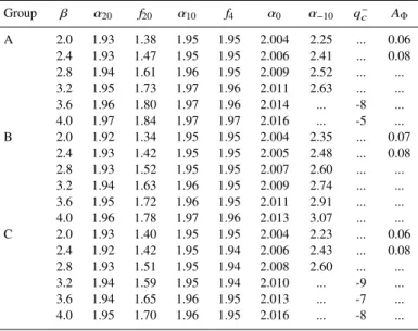
To complete this qualitative description of the computed MFS, let us look at the spectra of the fBm reference images, with particular emphasis to changes in the MFS as a consequence of variations of their fractal parameters. In Figure 7 the MFS, calculated for all the 18 images generated for this work (see Section 2.3 and Appendix A), are shown. The increase of the power-law exponent β clearly produces a systematic increase of the width of the q < 0 part, but also a drift of the extreme point of the q > 0 part towards larger values of f and α. This right-sided asymmetry indicates, in general, that small scale fluctuations exhibit a more pronounced multifractal behaviour than large scale ones. Again, let us notice that this overall trend does not exclude possible peculiar differences from image to image. Surprisingly, even for images generated with the same β (then with the same the fractal dimension, according to Equation 1) we can find differences depending on the choice of the random phases. It is possible to ascertain this fact comparing the shape of the MFS of images having the same β in the three panels of Figure 7, but corresponding to different random phase distributions. Finally, it is to notice that also the MFSs of the fBm images can suffer of the presence of cusp-like features, namely at the smallest negative q orders. Similarly to previously considered classes of images, in Table 4 the most relevant features of the MFS of fBm sets are listed.

Table 2.Main properties of the MFS of the analysed Hi-GAL frames. Field Band α₂₀ f20 α10 f4 α0 α−10 q+c AΦ `215 70 1.53 -0.64 1.56 1.72 2.001 2.01 ... ... 160 1.63 -0.06 1.65 1.77 2.006 2.12 ... 0.07 250 1.65 0.05 1.68 1.70 2.012 2.50 ... 0.12 350 1.64 -0.06 1.67 1.73 2.012 2.46 ... 0.12 500 1.70 0.22 1.73 1.76 2.014 2.50 ... 0.12 Column Density 1.66 0.23 1.68 1.71 2.014 2.52 ... 0.13 `217 70 ... ... ... -0.31 2.007 2.01 4 ... 160 ... ... ... -0.24 2.023 2.11 4 0.14 250 ... ... ... -0.12 2.031 2.47 5 0.18 350 ... ... ... -0.17 2.035 2.46 5 0.19 500 ... ... ... 0.22 2.035 2.41 6 0.19 Column Density 1.32 0.16 1.33 0.69 2.030 2.69 ... 0.17 `220 70 ... ... 1.21 -0.03 2.002 2.01 10 ... 160 ... ... ... -0.09 2.006 2.06 6 ... 250 ... ... ... -0.03 2.012 2.39 5 0.14 350 ... ... ... 0.03 2.013 2.39 6 0.14 500 ... ... ... 0.31 2.013 2.46 7 0.14 Column Density ... ... ... 0.67 2.012 2.47 8 0.13 `222 70 ... ... ... 1.57 2.002 2.01 9 ... 160 1.44 0.07 1.45 0.85 2.010 2.07 ... ... 250 1.41 0.00 1.41 0.89 2.020 2.45 ... 0.15 350 1.45 -0.06 1.45 1.08 2.021 2.44 ... 0.15 500 1.49 0.13 1.49 1.17 2.024 2.38 ... 0.15 Column Density 1.54 0.07 1.55 1.40 2.021 2.48 ... 0.14 `224 70 ... ... ... -0.38 2.005 2.02 4 ... 160 1.23 0.04 1.23 0.20 2.022 2.19 ... 0.13 250 1.24 -0.07 1.25 0.42 2.035 2.47 ... 0.18 350 1.31 0.07 1.32 0.71 2.044 2.57 ... 0.20 500 1.36 0.22 1.38 0.88 2.053 2.49 ... 0.21 Column Density 1.31 0.31 1.33 0.90 2.064 2.32 ... 0.20 `226 70 ... ... 1.25 0.18 2.001 2.00 12 ... 160 ... ... ... -0.21 2.007 2.04 5 ... 250 ... ... ... 0.08 2.021 2.33 6 0.14 350 ... ... ... 0.06 2.025 2.35 6 0.14 500 ... ... 1.35 0.61 2.026 2.27 10 0.14 Column Density ... ... 1.42 1.00 2.024 2.27 11 0.13

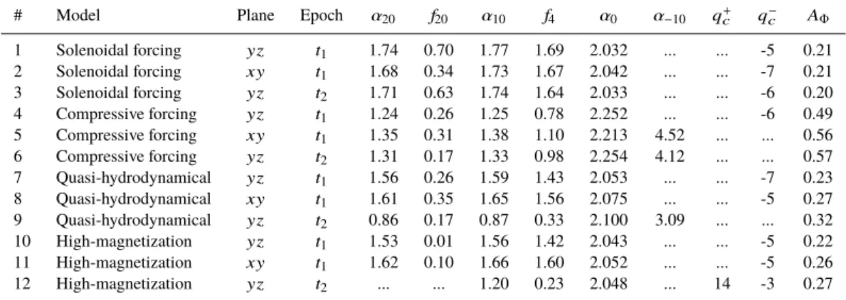
Table 3.Main properties of the MFS of the analysed simulations.

# Model Plane Epoch α20 f20 α10 f4 α0 α−10 q+c qc− AΦ

1 Solenoidal forcing yz t₁ 1.74 0.70 1.77 1.69 2.032 ... ... -5 0.21 2 Solenoidal forcing xy t₁ 1.68 0.34 1.73 1.67 2.042 ... ... -7 0.21 3 Solenoidal forcing yz t₂ 1.71 0.63 1.74 1.64 2.033 ... ... -6 0.20 4 Compressive forcing yz t₁ 1.24 0.26 1.25 0.78 2.252 ... ... -6 0.49 5 Compressive forcing xy t₁ 1.35 0.31 1.38 1.10 2.213 4.52 ... ... 0.56 6 Compressive forcing yz t₂ 1.31 0.17 1.33 0.98 2.254 4.12 ... ... 0.57 7 Quasi-hydrodynamical yz t₁ 1.56 0.26 1.59 1.43 2.053 ... ... -7 0.23 8 Quasi-hydrodynamical xy t₁ 1.61 0.35 1.65 1.56 2.075 ... ... -5 0.27 9 Quasi-hydrodynamical yz t2 0.86 0.17 0.87 0.33 2.100 3.09 ... ... 0.32 10 High-magnetization yz t1 1.53 0.01 1.56 1.42 2.043 ... ... -5 0.22 11 High-magnetization xy t1 1.62 0.10 1.66 1.60 2.052 ... ... -5 0.26 12 High-magnetization yz t2 ... ... 1.20 0.23 2.048 ... 14 -3 0.27

4.2 Quantifying the information contained in the MFS

In order to better quantify the information contained in the analysed MFSs, one needs to establish some meaningful descriptors of the geometry of the spectrum. The literature about multifractal analysis abounds with examples of such indicators. In the following discus-sion, we use a set of indicators which are independent of each other,

and/or are able to highlight common trends and differences among the analysed sets.

2.0

2.2

2.4

2.6

2.8

3.0

α

0.0

0.5

1.0

1.5

2.0

f

A

2.0

2.2

2.4

2.6

2.8

3.0

α

B

2.0

2.2

2.4

2.6

2.8

3.0

α

C

Figure 7.MFS of the fBm reference images reported in Figure A1, grouped by image phase distribution (cases “A”, “B”, and “C” in left, middle and right panel, respectively). A different color shade, from the darkest to the lightest, is used for indicating images with the power spectrum exponent β ranging from 2 to 4 in steps of 0.4.

Table 4.Main properties of the MFS of the analysed fBm images.

Group β α₂₀ f20 α10 f4 α0 α−10 q−c AΦ A 2.0 1.93 1.38 1.95 1.95 2.004 2.25 ... 0.06 2.4 1.93 1.47 1.95 1.95 2.006 2.41 ... 0.08 2.8 1.94 1.61 1.96 1.95 2.009 2.52 ... ... 3.2 1.95 1.73 1.97 1.96 2.011 2.63 ... ... 3.6 1.96 1.80 1.97 1.96 2.014 ... -8 ... 4.0 1.97 1.84 1.97 1.97 2.016 ... -5 ... B 2.0 1.92 1.34 1.95 1.95 2.004 2.35 ... 0.07 2.4 1.93 1.42 1.95 1.95 2.005 2.48 ... 0.08 2.8 1.93 1.52 1.95 1.95 2.007 2.60 ... ... 3.2 1.94 1.63 1.96 1.95 2.009 2.74 ... ... 3.6 1.95 1.72 1.96 1.95 2.011 2.91 ... ... 4.0 1.96 1.78 1.97 1.96 2.013 3.07 ... ... C 2.0 1.93 1.40 1.95 1.95 2.004 2.23 ... 0.06 2.4 1.92 1.42 1.95 1.94 2.006 2.43 ... 0.08 2.8 1.93 1.51 1.95 1.94 2.008 2.60 ... ... 3.2 1.94 1.59 1.95 1.94 2.010 ... -9 ... 3.6 1.94 1.65 1.96 1.95 2.013 ... -7 ... 4.0 1.95 1.70 1.96 1.95 2.016 ... -8 ...

4.2.1 Dimensional diversity vs maximum singularity strength

Here we start from the diagnostics adopted by Chappell & Scalo (2001), which permits a direct comparison with the unique previous case of MFS analysis of interstellar clouds (but with the limitation of considering only the left part of the MFS, neglecting the neg-ative q orders). These authors used α20as a measurement of the

strength of the brightest singularities found in a given map, and the f₄− f₂₀ offset (hereafter ∆ f_4,20) as a “dimensional diversity” to characterise their fields: an image containing isolated, strong and point-like concentrations will have low values of f for high q orders, while this parameter is expected to increase in presence of a large variety of geometries. These authors recognised an increasing trend in the ∆ f4,20 vs α20 scatter plot for their sample of IRAS-based

column density maps of 13 nearby star-forming regions, so that

structures with strong dominant concentrations (low α20) typically

have smaller dimensional diversities (low ∆ f4,20).

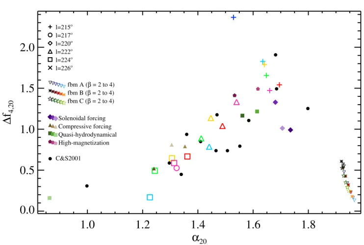
We extend this analysis to our data sets (Hi-GAL observations, simulations and fBm images) for which it was possible to compute the MFS up to q = 20 (see Tables 2 and 3, respectively). We find in Figure 8 that Hi-GAL and simulation maps follow the general trend delineated by the maps of Chappell & Scalo (2001). In par-ticular, among the Hi-GAL tiles, those present at various different wavelengths are `215, whose different bands occupy the upper part of such trend regardless of wavelength (except, again, for the com-pletely peculiar behaviour of the 70 µm map), `222 in the middle, and `224 at the bottom left end, where the column density map of `217 is found as well. In practice, the maps containing the strongest singularities, i.e. the most active star forming sites, `217 and `224, show not only, as expected, lower α values, but also a lower de-gree of dimensional diversity. Compared with the observational set

1.0

1.2

1.4

1.6

1.8

α

0.0

0.5

1.0

1.5

2.0

∆

f

Figure 8.Plot of “dimensional diversity”, expressed by ∆f_4,20 ≡ f (q= 4) − f (q = 20), versus the smallest computed value of the singularity strength α₂₀ ≡α(q = 20). Such quantities are available only for Hi-GAL maps with q+_c ≥20 . The correspondence of symbols and colors with tiles and bands, respectively, is explained in the legend; the symbol for the tile `226, although not present in the plot, is introduced since the convention established here is used also in other following figures. Points representing the the 12 cloud simulations and the 18 fBm images analysed in this work are plotted as well (symbols are explained in the legend). Furthermore, the positions of the 18 fBm reference images (located close to the bottom right corner of the diagram) are represented with smaller symbols, using color scales (different for the “A”, “B”, and “C” cases) to identify the different explored values of β. Finally, for comparison, points taken from Figure 8 of Chappell & Scalo (2001) and representing multifractal features of their IRAS-based column density maps of 13 nearby (d ≤ 160 pc) star forming regions are reported as filled black circles (“C&S2001”, in the legend).

of Chappell & Scalo (2001), their morphology appears, from the statistical point of view, similar to that of their L 134 and Cham 1 cases. On the contrary, tiles more quiescent from the point of view of the star ormation, such as `222 and `215, populate an upper region of the diagram. The latter, in particular, is found to be close to the positions of the fields Oph N, W, and U of Chappell & Scalo (2001), defined by these authors as the most “space filling” in their sample. The points representing models are spread along the same general trend, as well. Interestingly, the “solenoidal” case is found in the top-right part of the diagram, while the “compressive” one, characterised by stronger singularities, is found at smaller α20. For

both of them no particular dependence on projection or evolution-ary effects is seen. Also, both the “quasi-hydrodynamical” and the “high-magnetization” cases, at the time t1 populate the top-right

part of the diagram, but the evolutionary effect is strong in these cases, so that the corresponding MFS broadening seen in Figure 6 is mirrored in this diagram by a significant decrease of α20at t2,

which can be seen for the former model, while for the latter it can be guessed but not displayed because q+c = 14.

Finally, a surprising behaviour is seen for the fBm images in this diagram. They occupy a completely different region of the plot, corresponding to α20 > 1.9 and 0.1 < ∆ f4,20 < 0.6. This means

that, compared with both observations and models, these images

show at the same time a narrower right tail of the MFS, and a low content of fractal diversity. Inside the region occupied by these sets, a trend from top-left to bottom-right is observed at increasing β (so at decreasing fractal dimension). Anyway, all the fBm images appear segregated from the main trend of observational maps, and this should impose serious restrictions to the use of the fBm images as surrogate of the ISM maps, not yet highlighted in literature.

In fact, the assumed affinity between the fBm images and ob-servations of ISM is based on a certain visual similarity and the fact that the power spectrum of the latter ones exhibits a power-law behaviour and some randomness in the phase distribution (Stutzki et al. 1998). However, such a power-law is found only over a limited range of scales (e.g., Stutzki et al. 1998; Schneider et al. 2011), which is typical for natural fractals, and/or different slopes can be found in different ranges of spatial scale (Paper I). In particular, in Paper I it has been shown how strong departures from a single power-law behaviour appear if an original fBm image is manipu-lated to obtain a more realistic image, i.e. removing its periodicity, and/or easing off the emission along the borders of the image, and/or enhancing the emission in brightest regions to simulate the presence of strong overdensities (their Figure 3). Correspondingly, a change in the Fourier phases is expected as well. For example, Burkhart & Lazarian (2016), analysing numerical simulations of isothermal

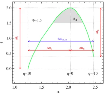
1.0 1.5 2.0 2.5 α 0.0 0.5 1.0 1.5 2.0 f q=10 q=0 q=-10 ∆α -10,10 ∆α L ∆αR ∆ fL ∆ fR AΦ Φ=1.5

Figure 9.Scheme of descriptors used to quantitatively characterize the MFS in this work, and introduced in the text. The example MFS (green curve) is the one of the `224 map at 250 µm, also contained in Figure 5.

compressible turbulence and focusing on information about phases, found that degree of coherence in phase distributions (being the co-herence equal to 0 in the case of a random distribution) depends on some simulation parameters, such as the sonic Mach number. Our present empirical analysis, therefore, highlights the need of a further comparative study of the phases among observational, numerical, and fBm maps.

4.2.2 Peak position

The analysis contained in the following represents an expansion of the Chappell & Scalo (2001) approach, thanks to the introduction of further diagnostics to describe the shape of the MFS. A graphic illustration of these quantities is also given, where possible, in Fig-ure 9.

Let us start with α0, namely the abscissa of the MFS peak: it is

lower if the signal is uncorrelated and the underlying process “loses fine structure”, i.e. the dominant fractal structure has more signal at larger fluctuations, since fine fluctuations become less frequent, so the object becomes more regular in appearance. In Table 2 a sys-tematic increase7is seen for α0from 70 to 500 µm for any Hi-GAL

tile. In particular, the largest gaps are seen between 70 and 160 µm, and from 160 µm to SPIRE wavelengths, while the column density maps show α0 values close to those of the SPIRE maps, with no

correspondence to a particular wavelength. The observed behaviour can be ascribed to the increasing degree of “structure” at increas-ing wavelength, namely a gradual enhancement of diffuse emission compared to isolated strong singularities. Furthermore, the most quiescent single tiles (`215, `220) show lower α0compared to the

others; in particular, at SPIRE wavelengths, they are characterized by α0 < 2.015, while α0 > 2.020 for the remaining tiles. No

systematic trends are found, instead, among different simulations

7 _{The differences among α0values are generally found on the second or the} third decimal digit (for this reason the precision of the α0values quoted in Tables 2, 3, and 4 is increased with respect to other analogous parameters). Despite this, they show interesting systematic trends.

2.00

2.02

2.04

2.06

α

0.4

0.6

0.8

1.0

1.2

1.4

∆α

Figure 10.Plot of the MFS “amplitude” ∆α−10,10versus the peak position α₀for the maps studied in this work for which a reliable α values in the the 10 ≤ q ≤ 10 range was derived. Data corresponding to the three turbulent ISM simulations with available ∆α−10,10(see Table 3) are all located at α₀ > 2.1 and ∆α−10,10 > 2.2 and are not displayed here not to overly compress the plot. The symbols are the same introduced in the legend of Figure 8.

(Table 3), except the remarkably large α₀values for the “compres-sive forcing” case, corresponding to a significantly more correlated signal, as already found, with respect to the “solenoidal forcing” case, by Federrath et al. (2009) through the structure function anal-ysis. Finally, a little but systematic increase of α0at increasing β is

seen for the fBm images (Table 4); notice indeed that for this class of objects, starting from the case β = 0 (white noise), corresponding to a totally uncorrelated signal, correlation increases with increasing β.

4.2.3 MFS width

A second relevant quantity is the MFS width, which expresses the degree of multifractality of the investigated set. The wider the range, the more multifractal are the fluctuations in the image. We express it here through the ∆α−10,10 ≡ α−10−α10parameter (see, e.g.,

Macek 2007). In Figure 10, this quantity is plotted versus α0 for

those maps having a MFS not involving cusps in −10 ≤ q ≤ 10. The considerations written above about α0are easily recognizable in the

abscissae of the points in the plot but, in addition, an interesting trend is seen between the two plotted quantities, with the degree of multifractality ∆α−_10,10generally increasing at increasing degree

of complexity expressed by α0. Such a trend is more easily

rec-ognizable for fBm images at increasing β, although confined to a shorter range of α0, than for Hi-GAL maps, whose corresponding

points are more scattered.

Another way to measure the amplitude of a MFS is to compute the area AΦdelimited by the MFS curve and a given horizontal cut

at a level f = Φ: AΦ=

∫ α_Φ,2

αΦ,1

[ f (α) − Φ] dα , (15)

where αΦ,1and αΦ,2represent the abscissae of the two points of the

0.4

0.6

0.8

1.0

1.2

1.4

∆α

0.05

0.10

0.15

0.20

A

Figure 11.Plot ot the area AΦunder the MFS and above f = 1.5 versus ∆α−10,10for maps for which both quantities can be derived. The symbols are the same introduced in the legend of Figure 8.

region, can be evaluated only for MFSs whose left and right tails are both intersected by the cut at f = Φ, which is formally expressed by the condition αmin< αΦ,1< αΦ,2< αmax. This also accounts for

the presence of possible cusp-like behaviour in the spectrum. The AΦobtained (choosing Φ = 1.5) for Hi-GAL fields, fBm sets and

simulations are quoted in Tables 2, 3, and 4, respectively.

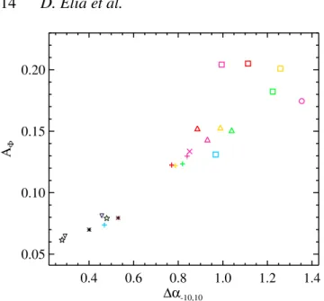
The correlation between AΦand ∆α−_10,10is investigated in

Figure 11, displaying a roughly linear correlation between these two descriptors, as expected, since an increase of the MFS width should correspond to an increase of AΦ, being the ordinate of the

MFS peak constant. Larger departures from this behaviour are seen at large values of these quantities, especially for 350 µm, 500 µm and column density images of `224. This indicates a particularly “swollen” shape of MFS, quite well recognisable in the `224 panel of Figure 5, especially for the colum density map. As in the case of Figure 10, in Figure 11 the points corresponding to simulations (three available cases: #5, #6, and #9 of Table 3) are not shown, being all of them located at ∆α−10,10> 2.2 and AΦ > 0.3, that is

to say far from the region of the plot populated by observational data sets, highlighting a different structure compared with real data. In particular, since both ∆α−_10,10and AΦ are descriptors of the

degree of multifractality in the signal, this indicates a generally wider variety of structures than observed in Hi-GAL tiles.

In our case, the benefit of using AΦ instead of ∆α−_10,10to

represent the MFS amplitudes consists of a larger number of useful maps. In Figure 12 the AΦversus α0plot confirms, based on a larger

sample of cases, the trends seen in Figure 10. The plot appears less scattered than that of Figure 10 with regard to positions of Hi-GAL and fBm images, while the positions of the simulations cover a wide range towards larger values. The “solenoidal” and the t1, yz

maps of both the “quasi-hydrodynamical” and “high magnetization” scenarios are the closest to the observational points, mostly to the ones corresponding to SPIRE maps of `224 and `217, that is to say that, from the point of view of the MFS amplitude, they show a degree of multifractality similar to that of the most actively star forming regions in our sample.

2.00

2.05

2.10

2.15

2.20

2.25

α

0.1

0.2

0.3

0.4

0.5

A

Figure 12.Plot ot the area AΦunder the MFS and above f = 1.5 versus the peak position α0for maps for which AΦcan be derived. The symbols are the same introduced in the legend of Figure 8.

0.0

0.2

0.4

0.6

0.8

1.0

1.2

∆α

0.0

0.5

1.0

1.5

2.0

∆α

Figure 13.Plot ot the MFS left versus right tail amplitude for maps for which it is possible to derive both quantities. The symbols are the same introduced in the legend of Figure 8. The dotted line represents the bisector, to facilitate the distinction between left-skewed (below the line) and right-skewed (above the line) MFSs, respectively.

4.2.4 Left vs right tail width

The diagnostics used in Figures 10, 11, and 12 consider the MFS as a whole, neglecting information contained in possible asymmetries. In fact, the left tail of the MFS represents the heterogeneity (broad tail) or uniformity (narrow tail) of the high values distribution, as well as the right tail is related to heterogeneity/uniformity of the low values distribution (e.g., Pavon-Dominguez et al. 2013; de Freitas et al. 2017). Strong asymmetries are observed in most of the spectra analysed in this paper, with the extreme case represented by PACS 70 µm maps, discussed above.

In order to make use of the MFS asymmetry, single values of α on the two sides of the MFS (for example, α10 and α−₁₀,