Air-sea interaction at contrasting sites in the Eastern Tropical Pacific : mesoscale variability and atmospheric convection at 10°N

Air-sea Interaction at Contrasting Sites in the Eastern

Tropical Pacific: mesoscale variability and atmospheric

convection at 10'N

by

J. Thomas Farrar

The University of Oklahoma S.M., Physical Oceanography, 2003

The Massachusetts Institute of Technology and the Woods Hole Oceanographic Institution

Submitted in partial fulfillment of the requirements for the degree of

Doctor of Philosophy

at the

MASSACHUSETTS INSTITUTE OF TECHNOLOGY

and the

WOODS HOLE OCEANOGRAPHIC INSTITUTION

February 2007

@2007 J. Thomas Farrar. All rights reserved.

The author hereby grants to MIT and WHOI permisson to reproduce and to distribute publicly copies of this thesis in whole or in part in any medium now known or hereafter created.

Author ...

Joint Program in Oceanography/A pplied Ocean Science and Engineering

Massachusetts Institute of Technology

Woods Hole Oceanographic Institution

November 15, 2006

Certified by ...

....

Robert Weller

Senior Scientist, W ods Hole Oc an~raphic Institution

/

/Thesis

Supervisor

Accepted by ... ...

Carl Wunsch

Chairman, Joint Committee for Ph sical Oceanography

Massachusetts Institute of Technology

Woods Hole Oceanographic Institution

MASSACHUSETTS IST E•

OF TECHNOLOGY

JUN 1 1 2007

ARCHVES

Air-sea Interaction at Contrasting Sites in the Eastern Tropical

Pacific: mesoscale variability and atmospheric convection at 10oN

by

J. Thomas Farrar

Submitted to the Massachusetts Institute of Technology and the Woods Hole Oceanographic Institution in partial fulfillment of the requirements for the degree of

Doctor of Philosophy

Abstract

The role of ocean dynamics in driving air-sea interaction is examined at two contrasting sites on 125°W in the eastern tropical Pacific Ocean using data from the Pan American Climate Study (PACS) field program. Analysis based on the PACS data set and satellite observations of sea surface temperature (SST) reveals marked differences in the role of ocean dynamics in modulating SST. At a near-equatorial site (3°S), the 1997-1998 El Niiio event dominated the evolution of SST and surface heat fluxes, and it is found that wind-driven southward Ekman transport was important in the local transition from El Nifio to La Nifia conditions. At a 10'N site near the summertime position of the Inter-tropical Convergence Zone, oceanic nmesoscale motions played an important role in modulating SST at intraseasonal (50- to 100-day) timescales, and the buoy observations suggest that there are variations in surface solar radiation coupled to these mesoscale SST variations. This suggests that the mesoscale oceanic variability may influence the occurrence of clouds.

The intraseasonal variability in currents, sea surface height, and SST at the northern site is examined within the broader spatial and temporal context afforded by satellite data. The oscillations have zonal wavelengths of 550-1650 km and propagate westward in a manner consistent with the dispersion relation for first baroclinic mode, free Rossby waves in the presence of a, mean westward flow. The hypothesis that the intraseasonal variability and its annual cycle are associated with baroclinic instability of the North Equatorial Current is supported by a spatio-temporal correlation between the amplitude of intraseasonal variability and the occurrence of westward zonal flows meeting an approximate necessary condition for baroclinic instability.

Focusing on 100_{N in the eastern tropical Pacific, the hypothesis that mesoscale oceanic}

SST variability can systematically influence cloud properties is investigated using several satellite data products. A statistically significant relationship between SST and columnar cloud liquid water (CLW), cloud reflectivity, and surface solar radiation is identified within the wavenumber-frequency band corresponding to oceanic Rossby waves. Analysis of seven years of CLW data and 20 years surface solar radiation data indicates that 10-20% of the variance of these cloud-related properties at intraseasonal periods and wavelengths on the order of 100 longitude can be ascribed to SST signals driven by oceanic Rossby waves.

Thesis Supervisor: Robert Weller

Acknowledgments

Most importantly, I would like to express my gratitude to my wife, Shelly, for her support, patience, and good humor during my graduate studies. Shelly's presence in my life has played an immeasurable role in my academic success and general well-being.

My parents, John and Ann, have done a great deal to instill in me the qualities that have allowed me to complete this research. Now that Shelly and I have our own son, John Oliver, I appreciate the efforts of my parents more than ever, and I hope that Shelly and I can do as well for John as my parents have done for me.

My advisor, Bob Weller, is a very busy scientist, but he has never been too busy to offer guidance when I have needed it. I feel lucky to have had the opportunity to have learned from Bob about the many important aspects of doing science, and I appreciate the special efforts he has made in this respect.

When fellow oceanographers ask who is on my thesis committee and I answer "Raf Ferrari, Jim Price, and John Toole", I am invariably told something to the effect of "Well, that's a good group". They certainly are a good group, and I feel very fortunate to have had the chance to interact with each of them. Besides being knowledgable scientists, each one is a kind person that I look up to. I am pleased to have received their advice on my research, but I am equally pleased to have been able to learn from them ways of talking about and conducting scientific research.

I am grateful to the many scientists and students at WHOI and MIT who gave me valuable input during the course of this work.

I (lid not take part in the collection of the mooring data, and I am indebted to Weller and the members of the Upper Ocean Processes (UOP) group whose committment to collection of high quality data is a valuable service to oceanography, meteorology, and society at large. All told, the mooring cruises required the efforts of 28 scientific crew and the ship's crew of three vessels. B.S. Way and W.M. Ostrom participated in all three cruises. Many others participated from shore in the preparation of instrumentation for the ships and moorings and in the data processing and compilation of data reports. The importance of these contri-butions to the present study cannot be overstated. The present study would not be possible without the scientific and managerial skill of chief scientists R. Weller and S. Anderson, the concerted effort of the members of the WHOI Upper Ocean Processes group, and funding the fieldwork by the National Oceanic and Atmospheric Administration (NOAA).

I gratefully acknowledge support from the following sources: NOAA Grants NA87RJ0445 (2002-2003) and NA17RJ1223 (2005-2006), and an MIT Presidential Fellowship (2000-2001). During 2005, I also recieved support from The Cooperative Institute for Climate and Ocean Research, a NOAA-WHOI joint institute (NOAA Grant NA17RJ1223). Although I was not involved in the data collection, the field experiment that made this study possible was conducted with support from NOAA (Grants NA66GPO130 and NA96GPO428). This work is done as part of the U.S. CLIVAR program.

Contents

1

1.1 Motivation ... ... 9

1.2 Thesis overview and driving questions ... ... 12

1.3 Organization ... ... .. 15

2 Data and Processing 17 2.1 Mooring Deployment ... . . 17

2.2 Instrumentation ... ... .. 18

2.3 Data Processing and Data Return ... ... 22

2.4 Estimation of Air-sea Fluxes ... ... 26

3 Observed Surface Layer Temperature Balance 29 3.1 Observed evolution of SST and surface heat flux . ... 29

3.2 Temperature balance approach ... ... 33

3.2.1 Theory ... ... .. 35

3.2.2 Estimation of terms ... ... 37

3.3 Results ... ... ... 43

3.3.1 Southern Site ... ... .. 43

3.3.2 Northern Site ... ... .. 46

3.3.3 Interpretation of the residual ... .... 47

3.4 Discussion ... ... . 49

4 Intraseasonal Variability near 100_{N in the Eastern Tropical Pacific Ocean}1 ₅₇ 4.1 Introduction ... ... .. 58

4.3 Intraseasonal variability at the mooring ... ... . 63

4.4 Intraseasonal variability near 10ON in the eastern tropical Pacific ... 71

4.5 Estimation of spatial scales and propagation characteristics ... 77

4.6 Discussion ... .. ... ... 83

4.6.1 Observed intraseasonal variability and the Rossby wave dispersion re-lation ... ... .. 84

4.6.2 Potential generation mechanisms . ... . 89

4.7 Conclusion ... ... .. 104

5 Cloud signals associated with oceanic Rossby waves on 10oN 107 5.1 Air-sea interaction at the oceanic mnesoscale ... .107

5.2 Data ... ... .... 109

5.3 SST fluctuations along 10'N in the eastern Pacific Ocean . ... 114

5.4 Time-space domain ... ... .. 114

5.5 Wavenumber-frequency domain ... ... 120

5.6 Discussion ... ... .. 132

Chapter 1

Introduction

1.1

Motivation

There are fundamental differences in the way the ocean and atmosphere influence one an-other. The ocean responds strongly to the atmospheric temperature, humidity, and winds at the surface, and the amount radiation impinging on the ocean surface depends strongly on clouds as well as water vapor and other aerosols. In contrast, the atmosphere responds primarily to the ocean's sea surface temperature (SST) field, which together with the atmo-sphere's surface properties, controls the flux of heat and water vapor across the sea surface. There is also a marked contrast in adjustment timescales of the ocean and atmosphere. In part because of the relatively large heat capacity and slow currents in the ocean, SST anomalies tend to evolve slowly in comparison to atmospheric temperature anomalies and can persist for months. Thus, understanding the processes that cause variations in SST is a high priority for those wishing to understand and simulate the evolution of the atmosphere at seasonal to climate timescales.

Air-sea interaction at large scales in the tropical Pacific has received a great deal of attention in the last several decades. The tropical oceans are recognized as an important component in setting the large scale atmospheric circulation. Solar heating of the ocean is maximal near the equator, and a substantial portion of this heat is transferred from the ocean to the atmosphere through latent, sensible, and longwave heat fluxes. The ascent of warm, moist surface air results in atmospheric deep convection in the Inter-tropical Convergence Zone (ITCZ) and constitutes a key part of the large scale meridional circulation in the

atmosphere. In addition, the zonal gradient of SST in the equatorial Pacific Ocean, because of its role in setting the basin scale atmospheric pressure gradient, is important to the maintenance of the trade winds. It is widely appreciated that fairly modest changes in tropical SST can lead to dramatic, planetary scale shifts in weather and the atmospheric circulation. El Nifio, which is characterized by an anomalous warming of the upper ocean of the eastern equatorial Pacific, is associated with a virtual shut-down of the trade winds and has profound impacts on global weather patterns.

Air-sea interaction at the oceanic mnesoscale is less well understood, but there has been much recent interest, partly as a result of satellite platforms that allow the long-term, high-resolution measurements required to adequately sample the oceanic mesoscale motions that occur on timescales of months and spatial scales on the order of 100 km. Since early ob-servations of mesoscale SST variability from space (e.g., Stumpf and Legeckis, 1977), it is now widely appreciated that SST signals and air-sea interaction at the oceanic mesoscale occur worldwide (e.g., Hill et al., 2000; Leeuwneburgh and Stammer, 2001; Xie, 2004; Small et al., 2005). Although satellite observations have been important in the realization of the global extent of oceanic mesoscale SST variability and associated air-sea interaction, in situ observations, though limited in time and space, have been instrumental in demonstrating that the air-sea interactions observed from satellites are not artifacts of the remote measure-ment techniques. For example, the identification of a relationship between the SST signal of tropical instability waves and surface wind speed in buoy data (Hayes et al., 1989) lent

confidence to subsequent studies of this relationship using satellite data.

The sea surface temperature field in the eastern tropical Pacific, with its strong asymme-try about the equator, energetic variability spanning weekly to interannual timescales, and links to climate is of great interest to those working to understand coupled ocean-atmosphere variability and the role of the tropical ocean in weather and climate variability. The eastern tropical Pacific is a prolific region of tropical cyclone generation, and recent studies suggest that the tropical Pacific SST distribution plays a crucial role in global climate anomalies (Cane, 1998; Shukla, 1998). The major oceanic and atmospheric circulations in the eastern tropical Pacific are strongly interdependent and are linked through the SST field. The strong meridional temperature gradient in the region spanning the eastern Pacific warm pool and the equatorial cold tongue is believed to influence the strength and location of the ITCZ (Lindzen and Nigam, 1987), and variability in the ITCZ may in turn influence the location

of the jet stream and precipitation over North America (Montroy, 1997). At the same time, the surface winds convergent on the ITCZ create an upwelling favorable wind stress pat-tern that exerts considerable influence on the strength and location of the North Equatorial Current/North Equatorial Counter Current current system (Kessler, 2002).

Our understanding of the processes that control SST in the eastern tropical Pacific is lacking due to sparse and incomplete observations, to uncertainties in identifying the relative roles of the various air-sea interaction and upper ocean processes, and to large errors in existing climatologies and gridded re-analyses of the surface heat flux, wind stress, and precipitation that might be used to drive ocean models. An important goal of field programs in the eastern tropical Pacific such as the Pan American Climate Study, the Eastern Pacific Investigation of Climate experiment, and the Tropical Atmosphere Ocean mooring array is to improve understanding of the processes that govern the evolution of SST with the ultimate goal of improving skill in prediction of the local and remote atmospheric variability driven by the SST field. Thus, there is strong motivation for understanding how ocean dynamics and ocean-atmosphere interactions and heat exchange work together to set the SST field in the eastern tropical Pacific. Of particular interest is identification and understanding of systematic relationships between SST, surface heat flux, and ocean dynamics.

The overarching goal of the Pan American Climate Study (PACS) cooperative field cam-paign has been to gain understanding of the relationship between SST variability in the tropical oceans and the climate of the American continents in order to improve the skill of seasonal-to-interannual climate forecasts. A thorough understanding of the processes gov-erning SST evolution in the region requires an account of the relative roles of local surface heat flux, freshwater flux, turbulent heat flux, and advection in determining SST and un-derstanding of how and why these factors vary through time.

As part of the PACS field program, two moorings were deployed on 125°W in the eastern tropical Pacific from May, 1997 to September, 1998 (Figure 1-1). One was placed at 100N in the eastern Pacific warm pool, near the northernmost climatological location of the ITCZ. The other mooring was placed at 30S in the Equatorial Cold Tongue. The primary goal of the PACS mooring deployment was to improve understanding of the processes that govern the evolution of sea surface temperature at two contrasting sites in the eastern tropical Pacific Ocean. The mooring time series have high vertical and temporal resolution of upper ocean temperature, salinity, and velocity and thus provide a unique opportunity to examine air-sea

Pacific climatological SST 300N 200N 100N 00 100S 200S 1200E 1500E 1800W 1500W 120°W 90°W Is I I I 19 21 23 25 27 29 C

Figure 1-1: The locations of the two PACS moorings. (Each mooring is indicated by an 'x'.) The climatological mean SST is also shown (Levitus and Boyer, 1994).

interaction and other processes that govern the evolution of the upper ocean.

1.2

Thesis overview and driving questions

This thesis uses data from the PACS moorings and satellite data to understand the relative importance of surface heat flux and ocean dynamics in setting SST during 1997-1998 and to examine the role of ocean dynamics in driving air-sea interaction. An initial goal in this thesis was to quantify the relative roles of surface heat fluxes, horizontal advection, and vertical mixing processes in setting SST at two contrasting sites in the eastern tropical Pacific using the high-quality PACS mooring data. The results of this initial effort led to further questions with interesting implications. The research path followed in this thesis is perhaps most clearly understood when the motivating questions are presented alongside with the results of the research motivated by those questions:

1. What are the relative roles of surface heat fluxes, horizontal advection, and vertical mixing processes in setting SST at the two PACS mooring sites?

At the southern site (near 3YS, 125'W), the evolution of SST and surface heat flux was dominated by a strong El Niflo event. The El Nifio event of 1997-1998 was, by some measures, the strongest one ever recorded (McPhadden, 1999), and it is unquestionably the most intensively studied El Nifio event. The upper-ocean temperature balance at the southern site allows some new insight into the role of wind-driven currents in the local establishment of the equatorial cold tongue at an off-equatorial site during the transition from El Nifio to La Nifia.

At the northern site (near 10'N, 125°W), the largest signal in the rate of change of SST at timescales longer than a few weeks was associated with quasi-periodic mesoscale motions

at intraseasonal periods (-40-100 days), and the temperature balance analysis suggested that the SST signal driven by these mesoscale motions may systematically affect air-sea heat exchange and atmospheric convection. While the buoy measurements of SST and solar radiation were suggestive of a causal relationship, the 17-month time-series from the mooring contained only a few cycles of the intraseasonal signal in velocity, SST, and heat flux. The questions below were prompted by closer examination of the strong intraseasonal variations in meridional velocity, SST, and surface solar radiation in this region, where few well-resolved in situ time series have been collected.

2. What is the dynamical nature of the quasi-periodic intraseasonal velocity

signal observed at the 10'N site? (Chapter 4)

The wavelike signal observed at the mooring site propagated westward and had a wave-length of about 550 kmn. Analysis of intraseasonal velocity variability on 100_{N in the broader}

spatial and temporal context afforded by satellite observations of sea surface height indicated that similar variability is characteristic of the region. The variability has previously been investigated from several different perspectives, and several distinct hypotheses have been put forward for its existence. This motivated a comprehensive study of the intraseasonal variability and an effort to resolve some of the contradictions between earlier studies.

The analysis shows that the intraseasonal variability tends to be strongest in the first part of each year, but its amplitude varies interannually. The intraseasonal velocity variability can be interpreted as being due to first baroclinic-mode Rossby waves under the influence of Doppler shifting by the mean westward flow. There is some evidence that baroclinic instability of the North Equatorial Current contributes energy to these westward-propagating

mesoscale disturbances, though the disturbances often appear to originate from the coastal regions near the Gulfs of Tehuantepec and Papagayo.

3. The buoy observations at the northern site further indicate that there is variability in solar radiation coupled to the mesoscale intraseasonal SST signal, which suggests that the oceanic mesoscale signal may modulate at-mospheric convection. Is there a systematic relationship between the SST expression of these mesoscale motions and atmospheric convection? (Chap-ter 5)

Yes, there is a systematic relationship between mnesoscale SST fluctuations within the Rossby wave band and some properties of clouds. Cross-spectral analysis of SST against satellite estimates of cloud liquid water and surface solar radiation indicates a statistically significant relationship at the wavelengths and periods corresponding to oceanic Rossby waves (identi-fied in addressing Question 2). Analysis of seven years of CLW data and 20 years of surface solar radiation data indicates that 10-20% of the variance of these cloud-related properties at intraseasonal periods and wavelengths on the order of 100 longitude can be ascribed to

SST signals driven by oceanic Rossby waves.

A relationship between cloud properties and mesoscale SST variations has been previously noted in the time-mean fields in the Agulhas Return Current region (near 45°S; O'Neill et al., 2005) and in association with tropical instability waves (Deser et al., 1993; Hashizume et al., 2001). This analysis extends those results by examining the relationship in wavenumber-frequency space, showing a broadband relationship (as opposed to a narrowband relationship associated with a particular wave or the time mean). In addition, this work shows that a common and widespread phenomenon, Rossby waves acting on a meridional SST gradient, can affect atmospheric convection. This study is also carried out in one of the worlds most active and important convective regions, and some work is done to show how mesoscale vari-ability in SST (more precisely, varivari-ability in surface heat and moisture fluxes) can modulate deep convection.

1.3

Organization

To the extent possible, each chapter is written so that it is a self-contained unit that can be understood without reference to the other chapters. The organization of this thesis is as follows.

The PACS mooring data are briefly described in Chapter 2. Readers not interested in the details of the mooring data collection and processing can skip Chapter 2. Several data sets derived from satellite observations are used in this thesis; these are described in the chapters in which they are used.

In Chapter 3, the observed evolution of SST and surface heat fluxes is presented, and the relative influence of surface heat fluxes, horizontal advection, and other processes in determining the evolution of upper ocean temperature is examined. Discussion focuses on the different roles of ocean dynamics at the two sites in contributing to horizontal advection and on the apparent coupling of surface heat fluxes with the local SST variability at the northern site.

In Chapter 4, the intraseasonal signal in meridional velocity is examined in its broader spatial and temporal context, and some important characteristics of the variability are quan-tified. The leading hypotheses for the variability are discussed and examined in light of these new insights into the characteristics of the variability.

In Chapter 5, the relationship between mesoscale SST variability and atmospheric con-vection, suggested by the buoy data at 10'N, is examined over a broader spatial and temporal domain using satellite-derived data. The interpretation of this relationship is discussed, and a hypothesis is advanced about how the resulting signal in solar radiation might feed back onto the upper-ocean temperature.

Chapter 2

Data and Processing

While this thesis utilizes several data sets, essential to this study are the high-quality moored measurements of upper ocean and surface meteorological properties that were collected as part of the NOAA-funded Pan American Climate Study (PACS) field project. This chapter addresses the collection and processing of the mooring data. Other data sets used in this thesis are described in the chapter in which they are used.

2.1

Mooring Deployment

From April 1997 through September 1998, air-sea interaction moorings were deployed near 100N, 125°W and 3WS, 1250W as part of the PACS field project (Figure 1-1). The northern mooring location was chosen because of its proximity to the climatological position of the ITCZ. The 30S, 125'W mooring site is within the region where the equatorial cold tongue normally appears, but the site was chosen to be south of the equator, which is routinely sampled by TAO moorings instrumented with current meters. The instrumentation on these moorings was selected to provide accurate time series of air-sea fluxes, surface meteorology, and upper ocean temperature, velocity, and salinity.

The initial deployment cruise was conducted aboard the R/V Roger Revelle from April 9 to May 5, 1997 (Way et al., 1998). A mid-term cruise was undertaken aboard the R/V

Thomas Thompson to recover, service, and re-deploy the moorings between November 28

and December 26, 1997 (Trask et al., 1998). Finally, the moorings were recovered from the

: i ,..,•.:•:5..PACS_{. . .. . i}

) I~

Figure 2-1: The PACS North buoy after deployment.

2.2

Instrumentation

The various sensors carried on the PACS buoys and mooring lines are described in detail by Anderson et al. (2000). The PACS moorings were heavily instrumented, often redundantly, both above and below the sea surface. On the buoy, an IMET (Improved METeorologi-cal) package provided measurements of wind velocity, air temperature, barometric pressure, relative humidity, precipitation, incoming short-wave radiation, and incoming long-wave ra-diation. Redundantly, a Vector Averaging Wind Recorder (VAWR) measured the same quantities. Below the surface, but mounted to the buoy in the upper 3 in of the ocean (Figure 2-2), there were seven independent temperature sensors and a SEACAT conductiv-ity/temperature sensor. In addition, sea surface temperature was measured using a floating temperature sensor. In the second phase of the field program, there were also stand-alone instruments to provide independent measurements of precipitation, relative humidity, and air temperature. Table 2.2 gives some details about the specific types of sensors used, their accuracy, and the averaging interval for the measurements.

'!za:L:-sea sur=ac eýere£az'4

:ers

Figure 2-2: Schematic showing the near surface field program (from Anderson, et al., 2000).

instrumentation for the second phase of the =IlDsure

--Parameter Sensor type Nominal accuracy Averaging

__t interval

Wind speed 3-cup Anemometer+ ±2% 15 min

R.M. Young 3-cup' ±5% 15 min

Wind direction Integral vane w/ vane ± 1 bit (5.6 15 min

follower' deg)

Insolation pyranometer' 3% 15 min

Incoming long-wave pyrgeometert ± 10% 15 min

radiation

Variable

dielectric

Relative humidity Variable dielectric 2% 15 min

conductor+

stand-alone/ASIMET*

±

± 0.2 mbar

Barometric pressure Quartz crystal' .when wind < 15 min 20 m/s

SST Thermistor' ± 0.0050C 15 nin

Thermistor 0.2C for

Air tezmperature _{"(unaspirated)' *wind > 5 m/s 15 min} stand-alone/ASIMET* 0.05 deg C 3.75 min

SEACAT 0.005oC7- 7.5 min

Subsurface temperature MicroCAT 0.0050C0 3.75 min

Brancker 0.0050CO- 30 min

VMCM 0.0050Cc 7.5 min

Conductivity SEACAT 0.01 psu 7.5 min

MicroCAT 0.01 psu 3.75 min

Vector current VMCM 1 cm/s 7.5 min

Precipitation RM Young rain guage 0.1 mm/hr 3.75 min Table 2.1: Table of measurement accuracies. I Part of VAWR package. *The stand-alone unit was deployed during phase 1 of the field study, while the ASIMET package was deployed during phase 2. @"In the laboratory, the accuracy is considerably higher, but this is the nominal accuracy that we estimate for field measurements.

sensors down to 200 m depth, Vector Measuring Current Meters (VMCMs; Weller and Davis, 1980) down to 110 m, and SEACAT conductivity sensors down to 80 m. For all sensors, vertical resolution was weighted toward the surface. The temperature sensors had the best vertical resolution, with about 30 sensors on the upper 200 nm. At deployment, salinity and velocity measurements had comparable resolution, with 8-10 sensors. Figure 2-3 depicts a typical mooring configuration for the PACS field program; there were differences in the sensor locations for each deployment at the two sites. (In this thesis, instrument depths will be noted as appropriate.)

Noe: All Sbackks down to a

Incding SpdhCL WS• wlNyli

Termnadoa to be Shot Pee.

TERMRYAWTON- CODEM

E not UW, rOIA W u-i VOaW16r COMM SWAIs

PON U-" CILtSW IRL 79S f N XCAMSL WU cS OSAMr~in&5ZL Df WCA UOcRL VI sulaux-Mmr~rp

ABRAM

t, WnALg VID 1IK r" ANCOe SACRLeS• 4

W"M"AIN Sla•CS S

w cAWnSUACM is a

A..

3 WmOmr Dism mey w VAWR m IMET, Beo&lW Arpt@oTarySeeT -Al•m RL

HamAfr TUp., StwMAa P.ecip, md

Plhled" Se Smrte T4e1oeSrsen Smmer 2111 miLS WIS &3i 33•VDT•L MI13WATWNO ,rinSL

3 .smpsr.Tarmmar, Legge rmw s rlrrl U MM RTenwameIWr CA-s Y4" Y Ce VMC 54 CIM T.s SEACAT ILTL3SYMIS CRAge s 3." Cage VIMCM uj T-POD wiLAmA l I SS CRr is 3M4 Capge MCM 157 SEACAT

3W Car S•sEVMCM ans cW Tvrsr

. I

WO 9uDe tlereage fr.ssm "rPso•sN

27J ACAT 3lM Y SMCWAIc

3* 3f" care V.MCM

3S T-POD/WirheClap *TI3E CfI

S3/4 Cope VMCM

a T-POD wlWirt Cmp . - - S6 U

ad Ali SECAT &74 L yr. e a cAn

is 3W car MM.4

ad S 0 OA'na - ,IT% be mla Si -r-.b

4 SEACAT i.

S 4"Cae VMCM

" T-POP wmi Chp ,_ r.. .0 1:2Wd 0o too wfffim TdPOD 21 HM _lbmp

ACOUSLC -ELEAS

ACOUSMI BETEAM

S. vr TrlU WI.a 1sr410 IW rl IPIAWLJ CHAIN

P.A.C.S. MOORING, 10" NORTH

Second Deployment

Figure 2-3: Schematic showing the mooring configuration for the second phase of the field program (from Anderson, et al., 2000).

i.A"Irn

WOO"=-~

I

2.3

Data Processing and Data Return

Details of the quality control and data processing can be found in Anderson et al. (2000), but some relevant aspects are presented here. The surface meteorological and current meter mea-surements were processed using software developed by the WHOI Upper-Ocean Processes (UOP) Group and pdeployment calibrations were applied to each instrument. When re-dundant measurements were available, inter-sensor comparisons were carried out, and efforts were made to determine which record was nmore reliable. Post-deployment calibrations were used when they produced better agreement in comparisons between redundant instrumenta-tion. All compass readings (surface and subsurface) were rotated as appropriate (by about 100) to correct for local magnetic deviation from true north. The processed data were visually inspected for sensor failure or gross errors. Sampling intervals for all instruments (including the meteorological packages) were 15 minutes or less. All of the data was averaged to a common 15 minute time base, and the data used here were further averaged to a 1-hour time base. In addition to post-processing carried out by Steven Anderson and others, a slight bias error (-0.1°C) in the 3.5 in subsurface temperature record during the second deployment at the northern site was identified (and corrected) by sensor inter-comparison during times when the temperature was believed to be vertically uniforlm.

Northern site

Two of the VMCMs ceased to produce meaningful data when the rotors failed on October 14, 1997 (20 and 40 m). The near simultaneous failure combined with the 20 m vertical separation between the two current meters suggests that a fishing vessel near the buoy ensnared the mooring with its lines. The problem was solved during the recovery and redeployment cruise on December 19, 1997 when the mooring was replaced.

Two of the Sea-bird SEACAT temperature and conductivity sensors also failed to produce data during the first phase of the field study (22.5 and 32.5 m). One was lost at sea, and the other was severely damaged. These two sensors were located between the two damaged current meters, and it seems likely that all four sensors were damaged by the same fishing vessel.

The floating SST sensor was also damaged during the first phase of the field program. The sensor was designed to follow the sea surface by floating up and down along stainless

steel rods. Upon recovery, one of the rods was bent, causing the sensor to remain out of the water. We believe that the rod was bent when a fishing vessel tied up to the buoy, possibly in order to pull the buoy to one side in order to catch fish that congregate around the mooring. The float functioned properly immediately after deployment and for the duration of the second leg of the field study.

Southern site

During the first deployment, two Brancker TPODs, a Sherman current meter, and a FSI acoustic current meter failed to return any meaningful data (depths of 35, 150, 120, and 130 m, respectively).

During the second deployment, two Seabird SEACAT (temperature and conductivity) sensors (1.5 m and 7.5 m) returned only partial records, extending to September 5, 1998 and July 2, 1998, respectively. In addition, three Brancker TPODs (0.5, 2.5, and 60 Im), a Sherman current meter (120 m), and a VMCM returned no data.

Salinity estimation

Some of the calculations in this thesis require knowledge of salinity at depths where salinity was not measured. At the northern site, damaged sensors during the first deployment limited the useful salinity information to only three depths in the upper 80 Im. At the southern site, the 1997-98 El Nifio caused the pycnocline to be deeper than anticipated during the first deployment, and thus the salinity measurements did not always span the pycnocline. Nonetheless, a large amount of salinity data was collected at each site; there were about 73,000 hourly estimates of salinity at the southern site and about 63,000 hourly estimates at the northern site. This subsection describes the procedure to estimate salinity at depths where it was not measured by taking advantage of the fairly close relationship observed between coincident measurements of temperature and salinity.

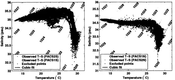
Scatter plots of salinity versus temperature (Fig. 2-4) suggest that salinity can be pre-dicted from temperature within 0.5 psu for temperatures less than about 260 (northern site) or 27°C (southern site). Temperatures higher than these thresholds correspond to temper-atures from the mixed layer during the rainy seasons, as indicated by the large range (up to 3 psu) of salinity observed at these temperatures. The anomalously large thermocline

35.5 35 3 34.5 • 34 m 33.5 33 32.5 -32 A" A S a. cc U) 15 20 25 30 15 20 25 30 Temperature ( C) Temperature ( C)

Figure 2-4: Observed temperature-salinity relationship (points) and cubic least-squares fit (red line). Left panel: southern mooring site. Right panel: northern mooring site. The black points were not used in the fit, and the rationale for their exclusion is explained in the text. Isopycnals, computed for a pressure of 50 db, are overlaid for reference (pink lines).

excursions associated with ENSO proved fortunate for this purpose, since this allowed sam-pling of a wide range of T-S values by a limited number of temperature-conductivity sensors. To take advantage of the relatively close T-S relationship at deeper levels, salinity was esti-mated by a cubic least squares regression approach. Before performing the regression, some "outliers" were removed from the southern record (near 23°C, 34.5 psu in Fig. 2-4) because inspection of the data revealed that these points were associated with an extreme shoaling of the thermocline (to about 17 m depth) during the La Nifia event and that the T-S relation during this time was clearly anomalous. In addition, temperatures exceeding 26 and 270C were excluded from the regression for the northern and southern sites, respectively. The resulting regression curves are indicated in Fig. 2-4.

One may question the usefulness of a cubic regression of salinity against temperature when the relationship shows appreciable scatter and a weak dependence of salinity on temperature. For example, would an assumption of constant salinity work just as well? One way to quantitatively measure of the utility of the fit is to assess the distribution of salinity values at a given temperature about the estimated regression curve, which allows an estimate of the likely error in salinity estimates inferred from the regression. Toward this end, T-S pairs were binned in 0.2'C by 0.02 psu bins to produce a histogram of the number of samples as a function of T and S. To obtain a normalized distribution of salinity values at a given

Observed T-S (PACS15) Excluded points . -- Cubic fit * ' ' r A w o. ._€ lu YL

Southern site

15

20

25

Temperature

(

C)

Northern site

34.8

3%

34.6

Z:

34.4

34

3.2

).15

1

05

15

20

25

Temperature

₍

_C)

Figure 2-5: Colored fields: Fraction of the total salinity observations within each temperature class (0.2'C bins) accounted for by each salinity class (0.02 psu bins). In other words, the total number of observations in each T-S bin has been normalized by the total number of observations within each temperature bin. Upper panel: southern mooring site. Lower panel: northern mooring site. The white line shows the cubic fit described in the text, and the error bars encompass 85% of the salinity observations at within each temperature bin (see text for details). Isopycnals, computed for a pressure of 50 db, are overlaid at 0.25 kg/m" intervals (pink lines) to allow visual assessment of the error in density associated with errors in salinity inferred from the regression.

0.2

1

05

.

3.2

).15

I I

temperature about the estimated regression curve, the number of samples in each bin was normalized by the total number of samples at each temperature (Figure 2-5). Then, the likely error in inferred salinity was assessed by computing the range of salinity about the regression curve that accounts for some fraction (85% was chosen here) of the total number of samples. The range of salinity values about the regression curve accounting for 85% of the observed salinity values is a function of temperature, and the maximum range is about 0.3 psu at both sites (Figure 2-5). (Note that the error bars in Figure 2-5 have been averaged over three adjacent temperature bins for clarity of presentation.) For these maximum errors, this corresponds to an uncertainty in density of about ±0.25 kg/m3 (Figure 2-5). The estimated errors are considerably smaller at other temperatures, typically ±0.2 psu or about ±0.125 kg/m3, and some of the error bars do not overlap, indicating that the cubic regression is a quantitative improvement on an assumption of constant salinity. Regression estimates of salinity are clearly inferior to estimates from direct measurements, but for calculations in this thesis, the resulting uncertainty in density is acceptable. Calculations using this regression (Chapter 3) will take account of the error inherent in this approach when assessing the significance of the results obtained.

2.4

Estimation of Air-sea Fluxes

The WHOI UOP Group used the surface meteorological and near-surface oceanographic measurements to determine the air-sea fluxes according to the TOGA COARE1 bulk flux algorithm of Fairall et al. (1996a). Although the algorithm includes corrections for 'cool skin' and 'warm layer' effects (cooling of the upper few millimeters and warming of the upper few meters of the ocean due to heat exchange), only the cool skin correction was employed in the flux calculations because the warm-layer correction is expected to be small as a result of the shallow (5 cm) measurement depth of the surface temperature.. The wind speed relative to the sea surface was calculated as the difference between the measured vector winds and the near surface current meter record. Full details of the air-sea flux calculations are given in Anderson et al. (2000).

The outgoing long-wave radiation (O(10pIm)) was estimated using the Stephan-Boltzmann

1

TOGA COARE stands for the Coupled Atmosphere Response Experiment of the Tropical Ocean-Global Atmosphere research program.

law, which can be expressed as P"E = caT4_{, where e is the sea surface emissivity (C}

= 0.97),

a is the Stefan-Boltzmann constant, and T is the sea surface skin temperature in degrees

Kelvin. The skin temperature is used because long-wave radiation depends on the interfacial temperature, which is slightly less than the temperature found about a millimeter below the surface (Saunders, 1967).

The precipitation rate was estimated by first-differencing measured accumulation in time. The R.M. Young rain gauge measures accumulated precipitation using a capacitance tech-nique to determine the amount of water in a collection chamber. Due to limited sample volume, the gauge siphons off the accumulated precipitation when the chamber is full. This process leads to spurious negative spikes in the precipitation rate, and these spikes were identified and replaced with zeros. Some additional noise in the precipitation rate was iden-tified, and we believe that this noise may be produced by electro-magnetic interference with nearby sensors (perhaps the Argos telemetry). The first-difference derivative may have also contributed to this noise. The noise appears to be about 0.1 mm/hr based on the noise about 0.0 nmmn/hr during times when the precipitation rate was known to be zero. Consequently, we rejected signals in the precipitation rate that were smaller than the estimated noise by setting precipitation rates less than 0.1 mm/hr to zero. The accumulated precipitation was then estimated as the time integral of the corrected precipitation rate.

The accuracy and applicability of the TOGA COAR.E bulk flux algorithm has been demonstrated in many contexts. The algorithm development involved simultaneous mea-surements from land stations, buoys, six research vessels, and 267 low-level airplane fly-overs (Weller et al., 2004). As a result of this intensive inter-comparison and inter-calibration campaign, measurement techniques and the bulk flux formulae were substantially improved, allowing the TOGA COARE Flux group to meet their goal of closing the monthly-average ocean heat and freshwater budgets to within 10 W/m2 and 20%, respectively (Weller et al., 2004). Since the TOGA COARE program, the Flux group has continued the coordi-nated effort to refine the bulk formulae and measurement techniques. Now, IMET surface fluxes, computed using the COARE flux algorithm, are being used for validation of other flux products (e.g. Shinoda et al., 1998; Shinoda and Hendon, 1998). Combined with accu-rate measurements of bulk surface meteorological properties, the TOGA COARE algorithm provides the best possible estimate of air-sea fluxes of heat, freshwater and momentum when direct covariance measurements of the fluxes are not available.

Chapter 3

Observed Surface Layer Temperature

Balance

In this chapter, the temperature balance of the surface layer is examined at each mooring site in order to allow quantitative estimates of the role of surface heat fluxes and horizontal advection in setting the temperature of the mixed layer on timescales longer than three weeks. Inferences are also made about the importance of vertical heat fluxes at the base of the mixed layer. Results regarding horizontal advection and surface heat fluxes at the northern site serve as the foundation for the remainder of the thesis.

The observed evolution of SST and surface heat flux is described in Section 3.1. Sec-tion 3.2 describes the method by which the surface layer temperature balance is estimated. Section 3.3 presents the results and is followed by a discussion (Section 3.4).

3.1

Observed evolution of SST and surface heat flux

The surface temperature record at the southern site was dominated by the El Nifio/La Nifia signal. SST was within about I°C of climatological values during during May 1997 but remained nearly steady during the boreal summer months when SST would normally be cooling (Figure 3-1). The largest deviation of SST from climatological conditions occurred in December of 1997, but temperatures continued to rise through April 1998. Peak El Nifio temperatures at the site exceeded 290_{C during March and April of 1998, and temperatures}

N E

X

z

(

Figure 3-1: Southern site (30S, 125'W). Upper panel: surface heat flux (3-week running average). Lower panel: SST (5 cm depth, hourly data) and Levitus and Boyer (1994) climatological SST.

This warm period was followed by a period of steadily decreasing surface temperatures; SST fell to about 24°C by mid-July of 1998.

As SST decreased in association with La Nifia (e.g., McPhaden, 1999), the net heat flux to the ocean increased markedly, reaching values in excess of 180 W/m2 by August of 1998 (Figure 3-1). Examination of the contributions to the net heat flux from latent, sensible, and radiative heat fluxes (Figure 3-2) reveals that this increase of the net heat flux during 1998 was due primarily to a marked decrease of evaporative heat loss as SST decreased. This tendency of surface heat flux variations to damlp interannual SST anomalies in the eastern

equatorial Pacific has been noted previously (Wang and McPhaden, 2001).

El Nifio did not have an obvious impact on the evolution of SST at the northern site.

SST was relatively warm in the the summers of 1997 and 1998, and it was coolest during January-May of 1998, as might be expected from the climatological seasonal cycle (Figure 3-3). The tendency for warm SST during the summer is closely linked with the presence of the ITCZ, which is associated with frequent precipitation and weak winds. When the ITCZ is south of the mooring site (roughly December 1997 through June 1998), the northeasterly

Ouu 250 200 150 100 m 50 0 -50 -100 -150 -200

250 n

Surface heat flux components at 3 S, 125°W

M J J A SO N D J FM AM J J A S

1997 1998

Figure 3-2: Surface heat flux components at the southern site. All quantities have been smoothed by a 3-week running average. Noteworthy features are: (1) latent and solar heat fluxes are the dominant contributions to the total heat flux, (2) the very warm El Niflo SST between December 1997 and May 1998 was accompanied by decreased (and variable) solar radiation and increased net-longwave radiation associated with enhanced atmospheric convection near the equator during that time, and (3) the contrast of El Nifto and La Nifia can be seen clearly in the difference in the latent heat flux between the summers of 1997 and 1998.

7

- Net heat flux

- -- Net solar - Latent -- Net longwave

---

I I I I I I I I I I I I I I I I I

(uI

E

cc

Figure 3-3: Northern site (10°N, 1250_{W). Upper panel: surface heat flux (3-week running}

average). Lower panel: SST (5 cm depth, hourly data) and Levitus and Boyer (1994) climatological SST.

trade winds are present at the site, contributing to strong, steady winds and enhanced evaporation. This seasonal variation of wind speed associated with the meridional migration

of the ITCZ contributes to seasonal variations in the size of the diurnal cycle of SST. The

decrease of wind speed and short wave radiation associated with the presence of the ITCZ represent competing effects on the size of the diurnal SST signal, but since the amount of diurnal warming depends more sensitively on the wind-stress magnitude than on surface heat flux (Fairall et al., 1996b), the diurnal cycle of SST is larger during the weaker winds of the ITCZ season.

One might expect the frequent convection and cloud cover within the ITCZ to block incoming solar radiation and reduce the net heating of the ocean, but the 17-month time series of net heat flux at the site shows that the heat flux was larger when the ITCZ was over the mooring site. Inspection of the individual components that make up the net heat flux suggests that the 21-day averaged solar heating is modulated by the presence of the ITCZ (Figure 3-4), but the increase in solar heating at the site associated with the southward migration of the ITCZ is no more than 50 W/rnm. This effect is overwhelmed by an increase

of evaporative heat loss from the sea surface as the humid, low-wind conditions of the ITCZ season give way to the drier, windier trade-wind season. The associated change in latent heat flux between August-October 1997 and January-April 1998 was roughly 100 W/m2_.

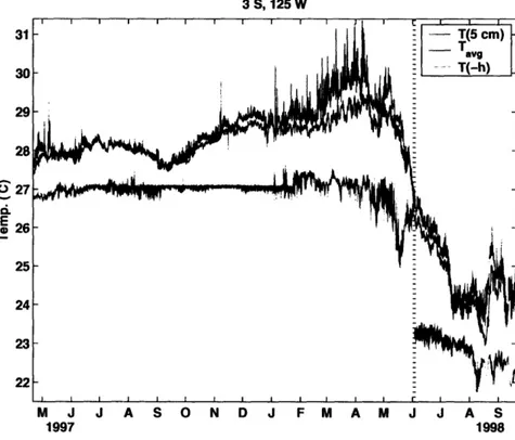
One feature that stands out during inspection of the net heat flux at the northern site is the presence of strong intraseasonal variability with a period of 40-70 days (Figures 3-3 and 3-4). This variability is present from January 1998 through the end of the record, and it has a magnitude comparable to that of the annual cycle. There are variations in SST at similar time scales. Contributions to this variability in the net heat flux come from variations in latent, sensible, and solar heat fluxes (Figure 3-4).

While inspection of the time series of SST and heat flux indicates that both sites exhibited coherent variability in SST and surface heat flux, better understanding of this relationship requires a quantitative measure of the importance of the surface heat flux in setting SST. Ex-amination of the mixed-layer temperature balance (below) allows quantitative understanding of the relative roles of surface heat fluxes, advection, and entrainment in setting SST, which, in turn, gives insight into the extent to which variations in heat fluxes are the cause or the result of the variations in SST.

3.2

Temperature balance approach

Excluding solar heating, heat that passes across the thin (0(1 mm)) diffusive-conductive boundary layer at the sea surface is carried to or away from the surface (depending on the sign of the surface flux) primarily by turbulent transport in the ocean boundary layer and serves to heat or cool the (typically) weakly stratified upper ocean. In part because it is difficult to measure a time series of the near-surface vertical turbulent heat transport, the role of the surface fluxes in setting upper-ocean temperature is usually assessed by comparing the rate of change of upper-ocean temperature, integrated from the surface to some depth, to the surface heat flux. Vertical integration across the boundary layer excludes from consideration the vertical turbulent heat flux within the boundary layer and places more emphasis on the role of turbulent transport at the integration depth.

The vertical integration of temperature (or heat) in the upper ocean can be carried out to a fixed depth (e.g., Emery, 1976; Merle, 1980) or to a depth that varies through time to track a physically meaningful surface like an isopycnal or the base of the mixed-layer

Surface heat flux components at 10oN, 1250W

E

M J J A S O

N D J

FM A M J

J A S

1997

1998

Figure 3-4: Surface heat flux components at the northern site. All quantities have been smoothed by a 3-week running average. Noteworthy features are: (1) latent and solar heat fluxes are the dominant contributions to the total heat flux, (2) the influence of the meridional migration of the ITCZ, which is near the mooring during the summer and fall months, can be seen clearly in the latent heat flux, and (3) intraseasonal variability (nominally 40- to 100- day periods) can be seen in every quantity except the longwave heat flux.

(e.g., McPhaden, 1982; Niiler and Stevenson, 1982). The fixed integration depth is often chosen to be below a strong thermocline so that the unknown vertical turbulent flux at the base of the integration volume can be assumed negligible (e.g., Price et al., 1978; Fischer et al., 2002; Weller et al., 2002). As discussed by Stevenson and Niiler (1983), carrying out the integration to a fixed depth below the thermocline does reduce the size of the typically unknown turbulent flux term, but, if the goal is to understand the evolution of SST, this approach has the potential disadvantage that the vertically averaged temperature may merely be a measure of the depth of the thermocline and may not be representative of SST. This is a concern in the tropical Pacific, where the thermocline is particularly strong. For example, consider an idealized case where the vertical thermal structure is represented by two layers with a thermocline at 50 m depth (meant to be representative of the eastern tropical Pacific). If the temperature change across the thermocline is 13'C, then a 10 change in mixed layer temperature changes the vertically averaged temperature less than a 5 m change in thermocline depth. The seasonal variation of SST over much of the eastern tropical Pacific is 1-3'C while changes in thermocline depth are 10-40 in, so the temperature integrated to a fixed depth below the thermocline is expected to be dominated by variations in the depth of the thermnocline. Thus, examination of the factors affecting temperature integrated to a fixed depth below the thermocline may not be the best approach for understanding the factors affecting SST.

In contrast, when the integration is carried out to a time-variable depth that tracks the base of the surface layer, the vertically averaged temperature should be a better measure of SST, to the extent that vertical variations in temperature are small above the integration depth. This approach is often employed for examination of the processes influencing tropical SST and upper-ocean heat content (e.g., Smyth et al., 1996; Cronin and McPhaden, 1997; Wang and McPhaden, 1999, 2001; Toole et al., 2004), and it is the approach employed here. This section describes the approach to estimation of the surface layer temperature balance at the two mooring sites.

3.2.1

Theory

A clear and complete derivation of the "heat storage rate equation" used for the temperature balance computation is given by Moisan and Niiler (1998); only a sketch of the derivation will

be given here. The derivation starts with the approximate equations governing conservation of heat and mass, i.e.,

OT OT OT OT OQ

pc,(

Ot Ox ay az 8z

= 0, _(3.2)

Ox Oy OZ

where the density (p) and the specific heat (cp) are treated as constants. The derivation proceeds by combining equations 3.1 and 3.2 and integrating vertically from some spatially and temporally variable depth h to the surface. Without further approximation, the equation governing the depth-average temperature between the surface and the depth h can be shown to be OTa 1 f 0 _{Ta - T, Oh QoQ} -

Q-h

where the subscript a indicates the vertical average to depth h, e.g.,

T, =h -J Tdz, (3.4)

and the 'hats' indicate deviations from the vertical average, so that, e.g., T(z) = T(z) + Ta. Equation 3.3 states that the rate of change of vertically averaged temperature (term A) is influenced by horizontal advection of the average temperature gradient by the layer-average velocity (term B), vertical entrainment (term D), and the net vertical divergence of vertical heat fluxes over the layer (term E). There is also a contribution to the vertically averaged temperature from a term associated with correlated vertical variations of temper-ature and velocity (term C), which has the form of the divergence of a Reynolds correlation (or 'eddy flux'). (Term C is not an 'eddy flux' in the conventional meaning of the term; that is, it is not associated with mesoscale or turbulent fluctuations, per se.)

Although Equation 3.3 follows mathematically from Equations 3.1-3.2 for any choice of

h(t), physical considerations suggest that if the "entrainment term" is to have its conventional

interpretation as being associated with mixing, then h should be chosen to follow an isotherm or an isopycnal rather than, for example, a mixed-layer depth chosen by a AT criterion.

When h is chosen as an isopycnal depth, the part of term D in parentheses is a diapycnal velocity (e.g. Pedlosky, 1998, pp. 100-102) and is nonzero only when there is mixing across the depth h.

Only some of the terms in Equation 3.3 can be directly estimated from available data. Thus it is helpful to manipulate Equation 3.3 further to explicitly separate the terms that can be directly estimated from those that cannot. The quantity Q-h (the heat flux across the depth h) contains contributions from penetrating solar radiation and from vertical turbulent

heat fluxes, which can be made explicit by writing Q-h = Qpen + Qturb. Equation 3.3 can then be rewritten as,

Ta

u

-VT

=

o

+

R,

_(3.5)

8t pcph

where

Qpe,,

1

- h (

-Qturb(

R= -IV

fiTdz +

Vh +

+

.

(3.6)

h -h h dt pcph

In the temperature balance calculation below, R will be inferred as a residual, and the other terms in Equation 3.5 will be estimated directly from data. The mixed-layer temperature balance equation (3.5) serves as the principal tool for analysis in this chapter.

3.2.2

Estimation of terms

This section describes the estimation of terms in Equation 3.5 for each mooring site. Many aspects of the estimation procedure are the same for the two sites, but differences in the evolution of upper-ocean temperature at the two sites requires the choice of the isopycnal defining h at each site to be considered individually. Thus, common aspects of the estimation procedure are described first, and then the choice of h is described for each site.

Aspects of estimation procedure common to both sites

At both sites, the horizontal gradient of Ta was estimated by a 4th-order accurate finite dif-ference scheme applied to multi-channel SST data from the Advanced Very High Resolution Radiometer (AVHRR) on the NOAA polar orbiting satellites (Brown et al., 1993). This data set has 18 km spatial resolution, but the data were averaged to 54 km resolution prior to computation of the gradients. The resulting estimate of the horizontal temperature gradient