How to Deal with Multi-source Data for Tree Detection Based on Deep Learning

HAL Id: lirmm-01685327

https://hal-lirmm.ccsd.cnrs.fr/lirmm-01685327

Submitted on 16 Jan 2018

HAL is a multi-disciplinary open access

archive for the deposit and dissemination of

sci-entific research documents, whether they are

pub-lished or not. The documents may come from

teaching and research institutions in France or

abroad, or from public or private research centers.

L’archive ouverte pluridisciplinaire HAL, est

destinée au dépôt et à la diffusion de documents

scientifiques de niveau recherche, publiés ou non,

émanant des établissements d’enseignement et de

recherche français ou étrangers, des laboratoires

publics ou privés.

How to Deal with Multi-source Data for Tree Detection

Based on Deep Learning

Lionel Pibre, Marc Chaumont, Gérard Subsol, Dino Ienco, Mustapha Derras

To cite this version:

Lionel Pibre, Marc Chaumont, Gérard Subsol, Dino Ienco, Mustapha Derras. How to Deal with

Multi-source Data for Tree Detection Based on Deep Learning. 5th IEEE Global Conference on Signal and

Information Processing (GlobalSIP), Nov 2017, Montreal, Canada. pp.1150-1154,

�10.1109/Global-SIP.2017.8309141�. �lirmm-01685327�

HOW TO DEAL WITH MULTI-SOURCE DATA FOR TREE DETECTION BASED ON DEEP

LEARNING

Lionel Pibre

_{, Marc Chaumont}

_{, G´erard Subsol}

_{, Dino Ienco}

_{and Mustapha Derras}

a

_{LIRMM laboratory, University of Montpellier, Montpellier, France;}

_{University of Nˆımes, Nˆımes, France;}

_CNRS;

_IRSTEA;

_{Berger-Levrault, France}

ABSTRACT

In the field of remote sensing, it is very common to use data from several sensors in order to make classification or seg-mentation. Most of the standard Remote Sensing analysis use machine learning methods based on image descriptions as HOG or SIFT and a classifier as SVM. In recent years neural networks have emerged as a key tool regarding the detection of objects. Due to the heterogeneity of information (optical, infrared, LiDAR), the combination of multi-source data is still an open issue in the Remote Sensing field. In this paper, we focus on managing data from multiple sources for the task of localization of urban trees in multi-source (optical, infrared, DSM) aerial images and we evaluate the different effects of preprocessing on the input data of a CNN.

Index Terms— Deep Learning, Localization, Multi-source Data, Data Fusion, Remote Sensing

1. INTRODUCTION

Nowadays, it is common to combine different information sources in order to deal with the object detection task [1] and more particularly in the field of remote sensing [2]. Indeed, it is admitted that the ”heterogeneity” of remote sensing infor-mation (optical, near-infrared, LiDAR) can improve the ob-ject detection.

In the case of multi-source data (optical, infrared, Li-DAR), it is nevertheless complex to merge several infor-mation sources since they provide measurements that can be different and complementary in their nature [3]. It is therefore crucial considering the integration issue during the concep-tion of an object detecconcep-tion method since, the way in which different data are combined can drastically impact the final result.

Recently, the Deep Learning [4] methods have shown that neural network models, and more specifically Convolutional Neural Networks (CNNs) are tailored to image classifica-tion[5] and localization [6]. CNNs [7] integrate in a single optimization schema both the learning of a classification model and the learning of a suitable set of descriptors of images.

CONTACT Lionel Pibre. Email:lionel.pibre@lirmm.fr

In this paper, we address the specific problem of localiza-tionand detection of urban trees in multi-source aerial data composed of synchronized optical, near infrared and Digi-tal Surface Model (DSM) measurements of urban areas. We should notify the reader that we are looking to localize each tree in the image. This task is more complicated than a simple global classification of an image. The task is also difficult due to the overlapping between trees. The task is an object detec-tion and not a pixel labelling which is also more complicated. The current approaches in the remote sensing field are of-ten ad hoc or heuristic [2]. In this paper, we propose to use CNN which indeed give a better solution. If we are looking for a more generalized problem of object detection, the so-lution is using CNN [8] but usually only with RGB images (and not near-infrared and/or DSM images) and the objects are often not overlapping or close.

Furthermore, we want to emphasize the importance of the image preprocessing when using a Deep Learning approach. Indeed, we try to demystify the CNNs by showing that the preparation of the learning data is of paramount importance on the performances of the CNNs.

The rest of the paper is organized as follows: Section 2 introduces CNNs and specifies the network architecture, Sec-tion 3 describes our approach. Experimental setting and re-sults are discussed in Section 4. Conclusions are drawn in Section 5.

2. DEEP LEARNING PRELIMINARIES A neural network [4] is a mathematical model whose design is inspired by the biological neurons. Initially, they were pro-posed to model the behavior of a brain. Since the 90’s, they have been used in Artificial Intelligence for learning purpose. Moreover, challenges such as ImageNet showed that these ap-proaches reached high classification performances [5, 9].

Neural networks are composed of different layers. The first layer is called the input layer, this layer is fed by the orig-inal data. The intermediate layers are called hidden layers and finally there is the output layer which returns the prediction. All these layers are composed of neurons that perform opera-tions on their input values (see Equation (1)).

σ_k(l)= x(l−1)_k · w(l)_k + b(l)_k (1) where σ(l)_k ∈ R is the result of the l − 1 layer, x(l−1)k ∈ R

are the neuron outputs coming from the l − 1 layer with k = {1, ..., K(l−1)_{} and w}(l)

k ∈ R are the weights.

In a convolutional neural network, hidden layers are com-posed of three successive processing: the convolution, the ap-plication of an activation function and finally the pooling.

The convolution of the first layer is a classical convolu-tion. The remaining convolutions are somewhat more spe-cific since the resulting images of these convolutions are the sums of K(l−1)convolutions, where K(l−1)is the number of outputs of the l − 1 layer.

After the convolution, a non-linear function called acti-vation function is applied to each value of the filtered im-age. The activation function may be a Gaussian function: f (x) = e−σ2x2, a ReLU [10] (Rectified Linear Unit): f (x) =

max(0, x), etc... These functions allow to break the linear-ity related to the convolutions. The pooling is an aggregation operation which reduces the dimension of the feature maps, and allows to reduce the number of calculations. This step is specific to convolutional neural networks. The two common methods employed to perform this operation are: i) the com-putation of the average (avg-pooling) ii) the selection of the maximum value among a local neighborhood (max-pooling). In addition, in an object classification task, the use of max-poolingallows a translation invariance of the features.

During the last decade, many network architectures have emerged. Among these, some networks have become popu-lar. They have become references of the state of the art. We present here one of these networks, AlexNet [9].

AlexNet [9] appears in 2012 during the ImageNet chal-lenge1_{. This network allowed Krizhevsky et al. to achieve}

the best performance on the ImageNet database. It consists of five convolutional layers. Each convolutional layer is fol-lowed by a ReLU [10] activation function and a max-pooling operation.

3. PROPOSITION

In order to locate the trees on the tested images, we used a multi-scale sliding window [11]. Since trees do not have the same crown diameter, this method allows us to detect all trees independently of the size.

As thumbnails images extracted from the sliding window must be of the same size than the images employed during the training phase, instead of varying the size of the sliding window, we vary the size of the tested images. We resize each image from 30% up to 300% of their original size with a step of 10%. The sliding window scans the tested images at every scale. Each thumbnail retrieved from the sliding window is given to the network which outputs the probability to contain

1_{http://www.image-net.org}

a tree. The network allows us to determine the area in the entire image that have a high probability of containing a tree. Applying our sliding window on the same image but at different scales will create an accumulation of bounding boxes over the same area. To overcome this problem we apply a fusion strategy on the set of overlapping bounding boxes classified as a tree. On all bounding boxes that overlap, we apply a strategy of fusion by area [12, 13].

The area fusion will compare all the pairs of bounding boxes. For each pair, we compute if one of the two bounding boxes overlaps each other by a percentage bigger than 80% (see equation (2)). If this is the case, the bounding box with the lowest probability of containing a tree is deleted.

Area(B1 ∩ B2)

min(Area(B1), Area(B2)) > 0.8 (2) with B1 and B2 two bounding boxes given by the network.Convolutions

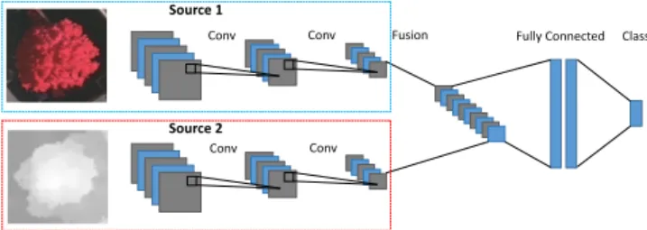
Convolutions Fully Connected Source 1 Source 2 Class Fusion

Conv Conv Fusion Fully Connected Class

Conv Conv

Source 1

Source 2

Fig. 1. Example of Late Fusion architecture. We also used the architecture proposed in [14]. The main idea of this architecture is to treat the different information in-dependently. This kind of architecture is called Late Fusion, an example is given in Figure 1. To construct this architecture, we used the well known AlexNet [9]. As seen in Figure 1, we duplicated the convolutional layers, and we concatenated the two branches before the fully connected layers. We can ob-serve from Figure 1 that the network has two inputs. Each entry corresponds to a different data type.

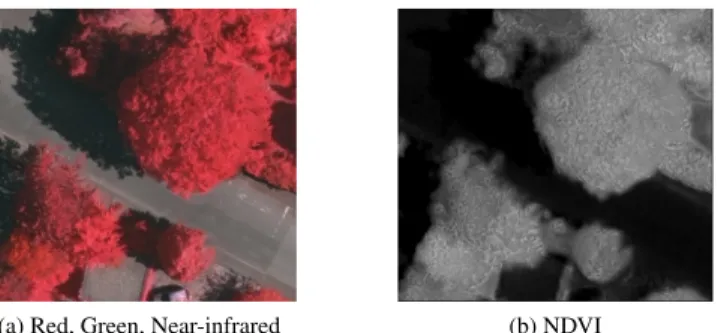
Moreover, we also used the Normalized Difference Vege-tation Index (NDVI) [15, 16]. This vegeVege-tation index is widely applied in the field of remote sensing [2]. This index allows to extract vegetation in images. The NDVI is a non-linear com-bination of red and near-infrared channels, see Equation 3.

N DV I = N IR − Red

N IR + Red (3) where Red and N IR stand for the spectral reflectance mea-surements acquired in the visible (red) and near-infrared re-gions, respectively.

We can observe Figure 2 that the NDVI allows us to re-move areas that are not vegetation. Thus, we can easily de-crease the number of false positives. Indeed, the different ob-jects that have a shape similar to that of a tree that are not vegetation are no longer present on the NDVI.

(a) Red, Green, Near-infrared (b) NDVI

Fig. 2. Generated NDVI from an Vaihingen dataset image.

4. EXPERIMENTAL RESULTS

In this section we report the experimental settings and we dis-cuss the results we obtained on the Vaihingen dataset. This dataset was captured over Vaihingen city in Germany2.

The RGNIR data were acquired using an Intergraph / ZI DMC flying 900m height above the ground with 9 cm ground resolution by the company RWE Power on 24 July and 6 Au-gust 2008 and a Digital Surface Model (DSM) with 9 cm ground resolution was interpolated from the AirBorne Laser Scanner point cloud acquired on 21 August 2008 by Leica Geosystems using a Leica ALS50 system with 45 field of view and a mean flying height above ground of 500m.

4.1. Experimental Settings

To train ours models we used a training base composed of about 6,000 ”tree” thumbnails and 40,000 ”other” thumb-nails. The thumbnail size is 64 × 64 pixels. The thumbnail images of the class “tree” are obtained by manual labeling of 19 entire images while the class “other” is obtained by ran-domly cropped images (that are not trees) of the 19 annotated images. In addition , to increase the number of thumbnails of the class “tree” (about 1,500 before transformation), we ap-plied rotations of 90◦, 180◦and 270◦to the thumbnails. Our test base is composed of about twenty images of variable size (from 125 × 150 pixels up to 550 × 725 pixels) and contains about a hundred trees.

To assess the results, we compute the overlap ratio be-tween the detected bounding box and the ground truth Eq. 4.

label =     

1 If area(detection∩ground truth)_{area(detection∪ground truth)} > 0.5

0 If area(detection∩ground truth)_{area(detection∪ground truth)} ≤ 0.5 (4) detection ∩ ground truth is the intersection between the de-tection and the ground truth, and area(dede-tection∪ground truth) is the union of their area.

2_{The Vaihingen data set was provided by the German Society for}

Photogrammetry, Remote Sensing and Geoinformation (DGPF) [17]: http://www.ifp.uni-stuttgart.de/dgpf/DKEP-Allg.html.

First, we tested a mono-band classification (only one source is used for the classification) but also by concatenating the R, G and NIR channels. These tests allow us to see among these different sources, which one is the most interesting to discriminate trees when used alone. Then we compare dif-ferent ways of integrating data from difdif-ferent sources into a CNN.

For the first way of integrating data from different sources, we have concatenated the different sources (EF Data1/ Data2), this kind of architecture is called Early Fusion (EF). We tested by concatenating the images RGNIR and DSM and finally we concatenated NDVI and DSM. For the last way of integrating data from different sources, we used the Late Fusion architecture described Section 3 (LF Data1/Data2). For these experiments we used the same pairs of data as for the Early Fusion architecture.

We want to remind the reader that our main objective is to show the impact and importance of data preparation when doing Deep Learning. To validate our experimentation, we perform a 5-fold cross validation.

4.2. Results and Discussions

Table 1, Table 2 and Table 3 summarize the results we have obtained on the Vaihingen dataset. They depict the average values of Recall, Precision and F-Measuremaxfor the

differ-ent models. We chose to take the point of the recall/precision curve where the f-measure is the highest.

4.2.1. Limits of using one only source

Table 1 shows the results we obtained using only one source. As can be seen the results between the different tests are very close. NDVI allows us to obtain the best performance in terms of Recall and F-Measuremax. The best Precision is

obtained using the DSM. It can be observed that the best re-sults in terms of F-Measuremaxare obtained when we have

transformed the original data, i.e. when we use the NDVI.

Table 1. Results using one source.

Source RGNIR DSM NDVI

F-Measuremax 60.45% 62.47% 63.97%

Recall 57.89% 57.62% 62.34%

Precision 63.44% 68.56% 67.04%

4.2.2. What is the best fusion process?

Table 2 shows the results we obtained using the Early Fu-sion. Here, we can see that the best results are obtained when using NDVI and DSM, we obtain a F-Measuremaxof 75%.

However, when we use RGNIR, the results are lower (67%). Table 3 shows the results that we have obtained using the Late Fusion architecture described in Section 3. The ob-servation is the same as in the previous experiments, better

Table 2. Results using multi-source data and the concatena-tion. EF RGNIR/DSM NDVI/DSM F-Measuremax 67.12% 75.30% Recall 65.40% 68.37% Precision 69.54% 84.11%

results are obtained when NDVI and DSM are used. When using NDVI and DSM, we obtain an F-Measuremaxof 72%

against 62% when using RGNIR and DSM. It can also be noted that this architecture gives lesser performances com-pared to the Early Fusion architecture.

Table 3. Results using multi-source data and the Late Fusion architecture.

LF RGNIR/DSM NDVI/DSM

F-Measuremax 62.14% 72.57%

Recall 62.54% 70.99%

Precision 62.65% 74.83%

The NDVI allows to keep only the essential informa-tion. Indeed the NDVI allows us to keep only the vegetation present in the image. This shows us the benefit of using a source which allows us to better discriminate trees, even if this source come from a heuristic transformation. In this case, it is possible that the lack of data prevents the networks to mix incorrectly the data.

Furthermore, we can observe that using DSM with NDVI gives much better results than just use the NDVI. Indeed, both are very important to detect and locate trees. If we detect an object that has a certain height and is vegetation, then there is a great chance that it is a tree. These two pieces of information are really crucial for detecting trees.

It can be noted that when using RGNIR alone, the result is not so far from those of NDVI or DSM. However, when we combine RGNIR and DSM the gain is not significant. Indeed, since these data are very different (their scale of value for example), it is very difficult for the CNN to discriminate trees correctly by concatenating these two types of data.

Moreover, we can observe that when we use the Late Fu-sion architecture the results are always inferior to the concate-nation. Indeed, when we use RGNIR and DSM the result goes from 62% to 67% while using the Early Fusion architecture. Similarly, when tested with NDVI and DSM, the results go from 72% with the Late Fusion architecture to 75% when using the Early Fusion architecture. Figure 3 shows two re-sults that we obtained.

4.2.3. How to select the sources to fuse?

Furthermore, we computed the correlation between each source using the Jaccard index. We compute the intersection

of trees found in two sources over the union of trees found in both sources. The results are presented Table 4. The second row of Table 4 represents the distribution of trees present only in one source.

Table 4. Results of the correlation between each source.

Sources RGNIR/DSM NDVI/DSM

Correlation 47.86% 48.96%

Distribution 26.47% 25.66% 28.75% 22.27%

We can observe that all the correlations are around 50%. These results show that among all the trees found, about 50% of the trees are found in both sources and therefore the re-maining 50% are found in either the first or the second source. Moreover, the second row of the table shows that the remain-ing 50% is distributed in the two sources and thus shows us the utility of combining several sources.

We also computed the correlation of false positives be-tween the different sources and we noticed that this corre-lation never exceeds 10% regardless of the sources studied. Thus, combining sources should reduce the number of false positives.

Fig. 3. Examples of the obtained results, in green we have the trees correctly localized, in blue the false negatives and in yellow the false positives.

5. CONCLUSION

In this paper, we have evaluated the use of Deep Learning methods to deal with multi-source data (optical, near-infrared and DSM). In addition, we have evaluated the impact of trans-formations applied to the input data of a CNN. We used the NDVI instead of using the data with the Red, Green and Near-Infrared channels. We realized our experiments on a problem of detection and localization of urban trees in multi-source aerial data.

Our work has shown that the use of NDVI allows to obtain the best performances and thus highlights the importance of the data that are used to learn a model with a CNN.

The results we have obtained set a milestone by showing the effectiveness of CNNs in merging different information with a performance gain exceeding 10%.

6. REFERENCES

[1] X. Liu and Y. Bo, “Object-based crop species classifica-tion based on the combinaclassifica-tion of airborne hyperspectral images and lidar data,” Remote Sensing, vol. 7, no. 1, pp. 922–950, 2015.

[2] M. Alonzo, B. Bookhagen, and D.A. Roberts, “Urban tree species mapping using hyperspectral and lidar data fusion,” Remote Sensing of Environment, vol. 148, pp. 70–83, 2014.

[3] M. Schmitt and X.X. Zhu, “Data fusion and remote sensing: An ever-growing relationship,” IEEE Geo-science and Remote Sensing Magazine, vol. 4, no. 4, pp. 6–23, 2016.

[4] Y. LeCun, Y. Bengio, and G.E. Hinton, “Deep learning,” Nature, vol. 52, no. 8, pp. 436–444, 2015.

[5] C. Szegedy, W. Liu, Y. Jia, P. Sermanet, et al., “Go-ing deeper with convolutions,” in IEEE Conference on Computer Vision and Pattern Recognition, 2015, pp. 1– 9.

[6] T. H. N. Le, Y. Zheng, C. Zhu, K. Luu, and M. Sav-vides, “Multiple scale faster-rcnn approach to driver’s cell-phone usage and hands on steering wheel detec-tion,” in 2016 IEEE Conference on Computer Vision and Pattern Recognition Workshops (CVPRW), June 2016, pp. 46–53.

[7] Y. LeCun, L.D. Jackel, L. Bottou, C. Cortes, J. S Denker, H. Drucker, I. Guyon, UA. Muller, E. Sackinger, P. Simard, et al., “Learning algorithms for classifica-tion: A comparison on handwritten digit recognition,” Neural networks: the statistical mechanics perspective, vol. 261, pp. 276, 1995.

[8] J.H. Bappy and A.K. Roy-Chowdhury, “Cnn based re-gion proposals for efficient object detection,” in Inter-national Conference on Image Processing (ICIP), 2016 IEEE International Conference on, Phoenix, Arizona, USA, September 2016, IEEE, pp. 3658–3662.

[9] A. Krizhevsk´y, I. Sutskever, and G.E. Hinton, “Ima-genet classification with deep convolutional neural net-works,” in Conference on Neural Information Process-ing Systems, 2012, pp. 1097–1105.

[10] V. Nair and G.E. Hinton, “Rectified linear units improve restricted boltzmann machines,” in International Con-ference on Machine Learning, 2010, pp. 807–814. [11] C. Garcia and M. Delakis, “Convolutional face finder:

A neural architecture for fast and robust face detection,” IEEE Trans. on Pattern Analysis and Machine Intelli-gence, vol. 26, no. 11, pp. 1408–1423, 2004.

[12] P. Sermanet, D. Eigen, X. Zhang, M. Mathieu, R. Fer-gus, and Y. LeCun, “Overfeat: Integrated recogni-tion, localization and detection using convolutional net-works,” in International Conference on Learning Rep-resentations (ICLR), Banff, Canada, April 2014. [13] M. Bertozzi, E. Binelli, A. Broggi, and MD. Rose,

“Stereo vision-based approaches for pedestrian detec-tion,” in IEEE Conference on Computer Vision and Pat-tern Recognition (CVPR), 2005, pp. 16–16.

[14] J. Wagner, V. Fischer, M. Herman, and S. Behnke, “Multispectral pedestrian detection using deep fusion convolutional neural networks,” in European Symp. on Artificial Neural Networks (ESANN), Bruges, Belgium, April 2016.

[15] G.E Meyer, “Machine vision identification of plants,” Recent Trends for Enhancing the Diversity and Quality of Soybean Products. Krezhova D (ed.) Croatia: InTech, 2011.

[16] A. Bannari, D-C. He, D. Morin, and H. Anys, “Analyse de l’apport de deux indices de v´eg´etation `a la classifica-tion dans les milieux h´et´erog`enes,” Canadian journal of remote sensing, vol. 24, no. 3, pp. 233–239, 1998. [17] M. Cramer, “The dgpf-test on digital airborne

camera evaluation–overview and test design,” Photogrammetrie-Fernerkundung-Geoinformation, vol. 2010, no. 2, pp. 73–82, 2010.