Application of robust statistics to asset allocation models

Application of Robust Statistics to Asset Allocation Models

by Xinfeng Zhou M.S., Chemistry

University of Washington, 2001 Submitted to Sloan School of Management

in partial fulfillment of the requirements for the degree of Master of Science in Operations Research

at the

MASSACHUSETTS INSTITUTE OF TECHNOLOGY June 2006 MASSACHUSETTS INSTTfUTE OF TECHNOLOGY JUL 2 4 2006 LIBRARIES ARCHIVES

@ 2006 Massachusetts Institute of Technology. All rights reserved

The author hereby grants to MIT permission to reproduce and to distribute publicly paper and electronic copies of this thesis in whole or in part

?2 _/)

Signature of Author

Author

...

of

/..I .v.

~~~'Signature

;. >.

...

...

a' c// Sloan School of Management

Operations Research Center May 2006

Certified

by ... ...

...

--

f-d Roy E. Welsch

Professor of Management Science, Statistics, and Engineering Systems Thesis Supervisor

Certified

by ...

... ... .

.... ...

George Verghese Professor of Electrical Engineering Thesis Supervisor

Accepted by ...

James B. Orlin Edward Pennell Brooks Professor of Operations Research Codirector, Operations Research Center

Application of Robust Statistics to Asset Allocation Models

By Xinfeng Zhou

Submitted to Sloan School of Management

On May 17, 2006 in partial fulfillment of the requirements for the degree of Master of Science in Operations Research

ABSTRACT

Many strategies for asset allocation involve the computation of expected returns and the covariance or correlation matrix of financial instruments returns. How much of each instrument to own is determined by an attempt to minimize risk (the variance of linear combinations of investments in these financial assets) subject to various constraints such as a given level of return, concentration limits, etc. The expected returns and the covariance matrix contain many parameters to estimate and two main problems arise. First, the data will very likely have outliers that will seriously affect the covariance matrix. Second, with so many parameters to estimate, a large number of observations are required and the nature of markets may change substantially over such a long period. In this thesis we use robust covariance procedures, such as FAST-MCD, quadrant-correlation-based covariance and 2D-Huber-based covariance, to address the first problem and regularization (Bayesian) methods that fully utilize the market weights of all assets for the second. High breakdown affine equivariant robust methods are effective, but tend to be costly when cross-validation is required to determine regularization parameters. We, therefore, also consider non-affine invariant robust covariance estimation. When back-tested on market data, these methods appear to be effective in improving portfolio performance. In conclusion, robust asset allocation methods have great potential to improve risk-adjusted portfolio returns and therefore deserve further exploration in investment management research.

Thesis Supervisor: Roy E. Welsch

Title: Professor of Management Science, Statistics, and Engineering Systems Thesis Supervisor: George Verghese

Acknowledgements

I would like to express my greatest gratitude to my advisors, Professor Roy Welsch and Professor George Verghese for their constant guidance, advice and encouragement. Working with Professor Welsch was a really rewarding experience. He truly shaped my understanding of statistics. Professor Verghese has been an inspiring mentor over the years who continuously encouraged and supported my efforts in knowledge-building and research. I am also deeply indebted to my PhD advisor, Professor Peter Dedon from the department of Biological Engineering Division, for his understanding and support over the last five years. I also want to thank Sameer Jain for his expertise, support and inputs into my work. Last but not at least, I would like to express many thanks to Dr. Jan-Hein Cremers at State Street Corporation for providing me opportunities to work on asset management projects and for inspiring my interests

in topics covered in this thesis.

Table of Contents

, Introduction of Asset Allocation Models ... 9

1.1 Overview ... 9

1.2 Foundation of Mean-Variance Portfolio Optimization ... 11

1.3 The Mean-Variance Efficient Frontier ... 15

1.4 Advantages and Disadvantages of Mean-Variance Optimization ... 20

2. Shrinkage Models and GARCH Models ... 22

2.1 Introduction ... 22

2.2 Sample Mean and Covariance Matrix ... 23

2.3 Factor Models ... 25

2.3.1 Single-factor Model ... 25

2.3.2. Multi-factor (Barra) model ... 26

2.3.3. Principal component analysis (PCA) ... 28

2.4. Shrinkage methods ... 29

2.5. Exponentially weighted moving average (EWMA) model ... 33

2.6. GARCH Model ... 35

2.6.1. Constant conditional correlation GARCH ... 39

2.6.2. Dynamic conditional correlation GARCH ... 40

2.6.3. BEKK GARCH ... 42

2.6.4. Scalar GARCH ... 42

2.7. Application to Historical Data ... 44

2.8. Conclusion ... 53

3. Robust Estimation of the Mean and Covariance Matrix ... 55

3.1. Introduction ... 55

3.2. Traditional Robust Estimators ... 56

3.2.1. LAD portfolio estimator ... 56

3.2.2. Huber portfolio estimator ... 58

3.2.3. Rank-correlation portfolio estimator ... 59

3.3. M-estimator ... 61

3.4. Fast-MCD ... 62

3.5. Pair-wise Robust Estimation ... 65

3.5.1. Quadrant correlation method ... 67

3.5.2. Two-dimensional Winsorization method ... ... 68

3.5.3. Two-dimensional Huber method ... 71

3.6. Application to Historical Data ... 73

3.7. C onclusion ... 80

4. Market-weight Bayesian Approaches ... 81

4.1. Introduction... 81

4.2. Black-Litterman model ... 83

4.3. Regularization models ... 87

4.4. Application of Regularization models ... 89

4.5. C onclusion ... 95

5. Summary and Future Research Directions ... 96

List of Figures

Figure 1.1. Efficient frontier and Capital Market Line

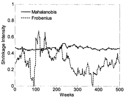
Figure 2.1. Optimal shrinkage intensity estimated using either Mahalanobis distance or asymptotic Frobenius norm estimation

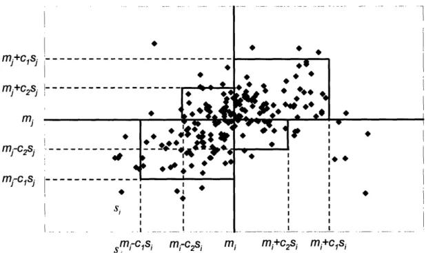
Figure 3.1. Adjusted Winsorization (for initial covariance) with c, = 1.96

List of Tables

Table 2.1. Application of shrinkage and GARCH methods

Table 2.2. Performance of V, CAPM, Principal, Mahalanobis, Frobenius, CCC-GARCH, DCC-GARCH models and Market index for up = 15%

Table 2.3. Performance of V, CAPM, Principal, Mahalanobis, Frobenius, CCC-GARCH,

DCC-GARCH models and Market index for p = 20%

Table 2.4. GMVP performance of V, CAPM, Principal, Mahalanobis, Frobenius, CCC-GARCH, DCC-GARCH models and Market index

Table 3.1. Application of robust estimation to expected returns and covariance matrix

Table 3.2. Performance of V, LAD, Huber, Rnakcov, FAST-MCD, QCIQR, 2D-Winsorization,

2D-Huber models and Market index for p = 15%

Table 3.3. Performance of V, LAD, Huber, Rnakcov, FAST-MCD, QCIQR, 2D-Winsorization, 2D-Huber models and Market index for p = 20%

Table 3.4. GMVP performance of V, FAST-MCD, QCIQR, 2D-Winsorization, 2D-Huber models and Market index

Table 4.1. Performance of V, V1, V2, LADI, LAD2, Hi, H2 models and Market index for

,p = 15%

Table 4.2. Performance of V, V1, V2, LAD1, LAD2, Hi, H2 models and Market index for

Chapter 1

Introduction of Asset Allocation Models

1.1 Overview

Asset allocation is the process that investors use to determine the asset classes in which to invest in and the weight for each asset class. Past studies have shown that asset allocation explains 75 -90°,' of the return variation and is the single most important factor determining the variability of portfolio performance. The objective of an asset allocation model is to find the right asset mix that provides the appropriate combination of expected return and risk that allows investors to achieve their financial goals. Harry Markowitz's mean-variance portfolio theory is by far the most well-known and well-studied asset allocation model for both academic researchers and practitioners alike (1, 2). The crux of mean-variance portfolio theory assumes that investors prefer (1) higher expected returns for a given level of standard deviation/variance and (2) lower standard deviations/variances for a given level of expected return. Portfolios that provide the maximum expected return for a given standard deviation and the minimum standard deviation for a given expected return are termed efficient portfolios and those that don't are termed inefficient portfolios.

Although intuitively and theoretically appealing, the application of mean-variance portfolio optimization has been hindered by the difficulty in accurately estimating model inputs, the expected returns and the covariance matrix of the assets. The goal of this thesis is to address this critical problem from different perspectives, with an emphasis on robust statistics and Bayesian

In Chapter 1, we first present the economic and mathematical background of the mean-variance portfolio optimization model and discuss the importance as well as the difficulty in estimating the model inputs, the expected return and the covariance matrix.

In Chapter 2, we investigate and apply some of the existing factor models and Bayesian shrinkage models as well as Generalized Autoregressive Conditional Heteroskedastic (GARCH) models to estimate the expected returns and the covariance matrix. Using the performance results of a US industrial selection portfolio, we show that "optimal" portfolios selected by shrinkage models have limited success when the number of assets N is of the same order as the number of return observations T. The GARCH models, which automatically include all historical information by exponential weighting, yield much better results.

In Chapter 3, we investigate and expand some of the robust statistical approaches to estimate the expected returns and the covariance matrix. Beside traditional robust methods, such as the least absolute deviation (LAD) method and the Spearman rank correlation, we focus more on recent developments such as the quadrant-correlation-based covariance and the 2D-Huber-based covariance to reduce or eliminate the effect of outliers. These new models prove to be more valuable than shrinkage models and GARCH models in dramatically improving risk-adjusted portfolio performance and reducing asset turnovers.

In Chapter 4, we investigate some of the more complex Bayesian approaches with emphasis on regularization models. We show that regularization models yield portfolios with significant increases in risk-adjusted portfolio performance, especially when transaction costs are taken into consideration. Our results also indicate that L₁ regularization methods may yield better results than L2 regularization methods. Overall L1 regularization methods also outperform the robust

covariance estimation methods (e.g., 2D-Huber), however the improvement is achieved at the cost of higher computational complexity.

Finally, in Chapter 5 we conclude this thesis by summarizing our results and offering possible directions for future research.

1.2 Foundation of Mean-Variance Portfolio Optimization

Mean-variance portfolio theory is built upon a basic economic principle, utility-maximization under economic constraints. In economics, utility is a measure of the happiness or satisfaction gained by consuming goods and services. Financial economists believe that rational investors make investment decisions (as well as consumption decisions) to maximize their lifetime expected utility under the budget constraints. The discrete version of the problem with T periods

can be mathematically formulated as:

MvIax EO[U(C, C2,", WT)] N

s.t. t+ t - Ct = n Pti (budget constraint)

iN ~ n (1.1)

Wt+l = It W tZt =(w, + IY - CtK)x tuitzi] (wealth dynamic)

where Wt, Wt+ are the wealth of the investor at time t and t+l, respectively; Yt is the (labor) income of the investor at period t; Ct is the consumption of the investor at time t; It is the

is the number of shares invested in the ith asset; wit nitit / It is the weight of the ith asset in the

n

portfolio, I wit = 1; Zit - Pit+l / Pit is the gross return of the ith asset.

i=l

The budget constraint equation states that the amount an investor can put into a portfolio is the amount of wealth at time t plus income minus consumption during the period. The wealth dynamic equation shows that the portfolio return equals the weighted average returns of individual assets in the investment.

The objective of this optimization problem is to maximize expected utilities over the lifetime of an investor. The utility function is a function of consumption and final wealth, which assigns a happiness score to each consumption set and final wealth. Different investors may have different utility functions; nevertheless the utility function of a rational investor should satisfy the following four basic properties:

1. Completeness: either Ul> U2 or U1< U2or U1 = U2;

2. Transitivity: U > U2, U2 > U3 = U > U3;

3. Non-satiation: more wealth/consumption is better than less wealth/consumption; 4. Law of diminishing returns: diminishing marginal utility of wealth/consumption.

Although the mathematical formulation is simple, the problem is a gigantic dynamic programming dilemma that can never be solved because all Yt, Pit, Zit and even Ct (which are

often influenced by inflation) are random numbers. Even for a small number of periods, the dimension of the problem becomes intractable.

Instead, a much simpler static version of the problem that only considers two time periods, 0 and 1, is often used in practice. The problem considers an investor with current wealth WO that needs to be invested in n assets, which will yield future wealth Wl. The utility at period 1 is determined

by W, and the simplified investment problem can be formulated as

Max E[U(W,)] N st. W = WO Wi ( + ri) i=l . N -w =1 i=1 (l.2)

where ri - P / P-1 is the net return of the ith asset; wi is the weight of the ith asset in the

portfolio. Again the weights of all assets add up to one, and the portfolio return is the weighted

average return of all the assets.

In this version of the problem, the utility function is a function of wealth level W, which reflects art investor's preferences and also reveals his/her attitude toward risk. Non-satiation indicates

dU

that investors prefer more wealth to less wealth, which means positive marginal utility: > 0

dW

d2U

V W. The Law of diminishing returns indicates that the utility function is concave, d < 0

V W. Power utility functions U = f(W) = 1 x Wr are commonly used by financial economists. A

log wealth utility function is a special case of the power utility. As y approaches 0, utility approaches the natural logarithm of wealth. A y equal to 1/2 implies less risk aversion than log

wealth, while a y equal to -1 implies greater risk aversion (3). Applying the second-order Taylor

series to any utility functions, we can express the utility as

U(W1) = U( 1) + U'()(W -W 1) + I U( 1)(W )2 + 1 U3 (W*)(W -W ) (1.3)

where W is the expected wealth at time 1; U'(W) and U "(WI)are the first and the second derivatives of utility function at W; U3(W*) is the third derivative of the utility function at

some W * between Wl and W.

If we approximate the function by ignoring the error term 1 U3(W*)(WI - W)3, E[U(W)] can be

written as E[U(W )] & U(W )+U'(W)E[(W -

l)]

This equation shows that if the expected wealth W, is held constant, the lower the variance the higher the expected utility since U"(W)< O0. If the variance is held constant, the higher the

expected wealth W the higher the expected utility since U '(W,) > 0.

Since U(W) is a monotone increasing function of Wl and W, = WO x (1+ E[rP]) is a monotone

increasing function of E[rp], U(W,) is also a monotone increasing function of E[rp]. The approximation indicates that investors prefer higher expected portfolio returns and lower

variance. We can represent the approximation using a quadratic utility function:

U = E[rP]- var(rp) (1.4)

where E[rp] is the expected portfolio return; var(rp) is the variance of the portfolio return; is the risk aversion coefficient ( > 0 ) with a larger value of A indicating higher risk aversion.

Ii the portfolio return follows a normal distribution, then E[(W - )3]=0 and the expected utility function is quadratic without approximation. So one underlying assumption behind mean/variance portfolio theory is that the portfolio return is normally distributed or investors have a quadratic utility function. It is worth noting that neither condition is met in reality. Simple quadratic functions may not be consistent with the fundamental property of a utility function since it indicates that, at certain wealth levels, the function has negative marginal utility and the investors prefer less wealth to more wealth (satiation). Asset returns often have fat tails and/or are positive/negatively skewed. So mean-variance optimization, as many other mathematical models, is a simplified representation of reality.

1.3 The Mean-Variance Efficient Frontier

For a portfolio with N risky assets to invest in, the portfolio return is the weighted average return of each asset: rp-wir, + w₂r₂+ + wNrN = w'r. So the expected return and the variance of portfolio can be expressed as

,Up = WI/J + W2,2 + . + WNPN = W'

N (1.5)

var(rp) _ var(wlr + w2r2 +.+ wNrN) = 22 + jwiwj =w'w (1.5)

i= izj

where wi, Vi = 1, N is the weight of the ith asset in the portfolio; ri, Vi = 1, ,N is the return

of the ith asset in the portfolio, r Pi /Pio -1; i, Vi = 1,* *, N is the expected return of the ith

is a Nx 1 column vector of ui s; E is the covariance matrix of the returns of N assets, an Nx N

matrix.

Since the optimal portfolio minimizes the variance of return for a given level of expected return, we can formulate the following problem to assign optimal weight to each asset and identify the efficient portfolio:

min w'Zw

a2

(1.6)

s.t. w'e = iUp, w'e = 1

where e is N x 1 column vector with all elements 1.

This problem can be solved in closed form using the method of Lagrange (4):

L = w'Zw + y(up - w',u)+ (1- w'e) where 2 is a l x k vector.

To minimize L, take the derivative of w, y and 2

<: w-yu-e=O

C - tpB

D

(Minimum varinace portfolio)

(1.7)

where A = e'-e > O, B = e'Y-',u, C = ,u'-lu > 0, D = AC-B 2_.

For each specified u , we can easily derive the optimal portfolio weights w* and the corresponding minimum variance ap = w*'Ew*. Combining the results, we have a hyperbola

2p=A+y p =A 2 -2B#p +CD , which describes the relationship between the expected

return and the standard deviation.

aL =0O aL =0 ay 0L =0 I I

To minimize the variance, set d(v )l/dup=O, and we have the global minimum variance portfolio:

jug =BIA => 7 =1/A, w = Z-e/A. (1.8)

As the result clearly shows, the global minimum variance portfolio (GMVP) does not require an estimation of expected returns u , which makes it a perfect choice to independently test covariance matrix estimation.

If a riskless asset (an asset with zero variance) with return rf is introduced, the problem becomes:

min w'Zw_{. 2}

w

s.t. w'u +(1-w'e)rf =up

Again using the Lagrange method, we have

1'* = - ( - rf e) and = ip -rf

(u - rfe)T -l ( - rfe)

ap - rf

C-2rfB+rf2A

The relationship between expected portfolio return and the variance of efficient portfolio can be

expressed as:

2 =(up - r)2/

c.P

/E,E=C-2rfB+rfA=(a-rfe)'Z-l(/u-rfe)

The equation is more frequently expressed as Sharpe ratio= P -rf =,

ap

which is the

foundation of the well-known Capital Asset Pricing Model (CAPM) introduced by Sharpe and

Lintner (5, 6).

Borrowing rm rF Efficient ;rontier , Gp CTm

Figure 1.1. Efficient frontier and Capital Market Line

As shown in Figure 1.1, the relationship between the expected return and the risk (as measured by standard deviation) is a linear relationship. The addition of a riskless asset changes the hyperbolic efficient frontier to a straight line, which is tangent to the efficient frontier with only risky assets. It shows that investors should only invest in a combination of the risk free asset and the tangent portfolio. Under a set of strict assumptions, such as perfect rationality and homogenous expectations of investors, Sharpe and Litner showed that the tangent portfolio must be the market portfolio (a value weighted index of the entire market) and the tangent line is called the capital market line (CML). The mathematics behind this is complex, but the intuition is straightforward. In equilibrium, all stocks must be held (markets have to clear). Therefore, prices will adjust to make sure that holding the market portfolio is the best choice. This result is often referred to as CAPM since it provides a prediction of the relationship between an asset's risk and its expected return. Based on CAPM, the expected excess return of any asset can be expressed as a function of market return:

,-rf

i(E[r]-rf)

(1.12)

where , = cov( arm) P,,m x is the sensitivity of the asset returns to the market returns;

var(rm) Om

E [rm] is the expected return on the market portfolio.

CAPM decomposes an asset's risk into systematic risk and idiosyncratic risk. Systematic risk is determined by the covariance of the asset with the market portfolio, and the rest of the risk is idiosyncratic risk. The gist of CAPM is that only systematic risk will be compensated with higher expected return, while idiosyncratic risk is not compensated since it can be diversified away. US treasury bills are often considered to be a risk-free asset for US investors. The market portfolio is supposed to include all risky assets. Yet in practice, S&P 500 and other traditional market-weighted indices are often used as a proxy for the market portfolio.

Legal restrictions, investment policies and investors' attitudes often impose constraints on the assets classes to invest in as well as portfolio weights. One of the most common constraints is to exclude short sales ( w_i 0, i = 1, , N ), which is the legal requirement of many mutual funds and pension funds. Taking different constraints into consideration, a more general portfolio optimization problem can be expressed as:

min w' Zw 2

Jt. W, P ='Up (1.13)

Aw>c

Bw=d

where Aw > c represents the inequality constraints of asset weights and Bw = d represents the equality constraints.

The problem is a quadratic minimization problem with linear constraints. The necessary and sufficient conditions for the problem are given by the Kuhn-Tucker conditions. All these optimization problems can be solved efficiently using quadratic programming algorithms, such as the interior point method.

1.4

Advantages and Disadvantages of Mean-Variance

Optimization

The simple mean-variance optimization only requires the expected return vector and expected covariance matrix as inputs. Factors such as each individual's preference become irrelevant. The model is based on a formal quantitative objective that will always give the same solution with the same set of parameters. So the model is not subject to investors' biases due to current or past market events. Also, the formation can be solved efficiently either in closed form or through numerical methods. These all explain its popularity and its contribution to modem portfolio theory (MPT).

However, some of the underlying assumptions of mean-variance portfolio optimization are open to question. For example, the utility function might involve preferences for more than the mean and variance of the portfolio returns and might be a complex function in which a quadratic approximation is not appropriate. Financial asset returns often do not follow normal distribution. Instead, they are often skewed and have fat tails. When the asset return is skewed, it is also arguable whether variance is the correct risk measure since it equally penalizes desirable upside and undersirable downside deviations from the mean. Two alternative measures of risk, semivariance and shortfall risk are sometimes used. The semi-variance of portfolio return rp

with mean ,up is defined as 2emi = E[(,p - rp )-]2, where the expectation is taken with respect to the distribution of rp, and where (,up- rp)- = ,-rp if rp <,up and 0 otherwise. The shortfall risk of a portfolio is defined as sa (w) = ,up - E[rp rp < qx (w)] where

q~ (w) = inf{z I P(rp < z) > a} is the a-quantile of the portfolio. Besides, the one-period nature of

static optimization also does not take dynamic factors into account, so some researchers argue for more complicated models based on stochastic processes and dynamic programming.

However, the most serious problem of the mean-variance efficient frontier is probably the method's instability. The mean-variance frontier is very sensitive to the inputs, and these inputs are subject to random errors in estimation of expected return and covariance. Small and statistically insignificant changes in these estimates can lead to a significant change in the composition of the efficient frontier. This may lead us to frequently and mistakenly rebalance our portfolio to stay on this elusive efficient frontier, incurring unnecessary transaction costs. The traditional Markowitz portfolio optimization estimates the expected return and the covariance matrix from historical return time series and treats them as true parameters for portfolio selection. This "certainty equivalence" view has long been criticized because of the impact of parameter uncertainty on optimal portfolio selection (7-9). The naive mean-variance approach often leads to extreme portfolio weights (instead of a diversified portfolio as the method anticipates) and dramatic swings in weights when there is a minor change to the expected returns or the covariance matrix. As a result, the practical application of the mean-variance optimization is seriously hindered by estimation errors. In the following chapters, we will discuss a variety of more sophisticated approaches to address the estimation error problem and to increase the risk-adjusted portfolio performance.

Chapter 2

Shrinkage Models and GARCH Models

2.1 Introduction

As discussed in Chapter 1, the correct estimation of expected returns and the covariance matrix is

a crucial step for asset management. Small estimation errors of either input usually lead to a

portfolio far from the true optimal efficient frontier. Besides asset allocation, the expected

returns and the covariance are also widely used in risk management (e.g. value at risk),

derivative pricing, hedging strategies and tests of asset pricing models. Naturally extensive studies have been conducted on their estimation and a variety of methods have been published to tackle the estimation error problem from different angles. Many of the methods address the questions as to how much structure we should place on the estimation. Since equally-weighted sample mean and covariance matrix have the desired property of being unbiased (the expected

value is equal to the true covariance matrix) and are easy to compute, they still are the most

widely used estimators in asset management. Despite the simple computation involved, this model has high complexity (large number of parameters), so the model suffers from the problem of high variance, which means the estimation errors can be significant and generate erroneous mean-variance efficient frontiers. The problem is further exacerbated if the number of observations is of the same order as the number of assets, which is often the case in financial

applications to select industry sectors or individual securities.

Besides the "data-based" approach, which assumes a functional form for the distribution of asset returns and estimates its parameters from the time series of returns, an alternative "model-based"

approach imposes a strong structure on the returns, assuming the returns are explained by a number of risk factors. A typical example is the single-factor model based on CAPM, where the expected returns and covariance of assets are believed to be determined by the market beta. This model has low variance in estimation, yet the model may fail to capture the complexity of the relationship between different assets and, as a result, the estimation can be severely biased. More recent research has focused on finding the right tradeoff between the sample covariance matrix and a highly-structured estimator using shrinkage methods, which will be investigated in the first half of this Chapter.

Neither the market model approaches nor the shrinkage methods address the well documented facts that high-frequency financial data tend to substantially deviate from the Gaussian distribution, and the expected returns/covariance matrix is influenced by time dependent information flows. Time series models, especially exponentially weighted moving average models and GARCH models, extract more information from the time series and have the potential to rectify (at least part of) the problem. So in the second half of this Chapter, we will discuss and implement some of the multivariate GARCH models developed over the past decade and evaluate their potential values in asset management.

2.2

Sample Mean and Covariance Matrix

For all our studies, we denote R as a T x N matrix, where each column vector R.i, i = 1,...,N represents a variable and each row Rt., t = 1,... ,T represents a cross-sectional observation. For

historical return data, each column R.i represents the returns of asset i over different periods, each row R. represents the returns of different assets at period t. For convenience, we also

denote Rt = R. as a Nx _te column vector for returns of different assets at period t and rti ( or rt,i)

as the return of asset i at period t.

The simple sample mean and covariance matrix are the best unbiased estimators using the maximum likelihood method under the assumption of multivariate normality. The covariance matrix can be calculated as

S=

(X-eR ')'(X-eR ') = T-l R'(I-ee')R

(2.1)

T-l

T-1

T

T

where R is a Nxl sample mean vector with = rtj; e is a Txl vector of ones; I is a

t=l

Tx T identity matrix;

Besides its intuitive interpretation, the sample mean and the sample covariance matrix require trivial computation. However the number of the parameters estimated is N(N + 3) / 2. When the number of assets is large relative to the number of historical return observations available, the sample covariance is often estimated with a lot of error. One natural solution to address this problem is to use a long historical period with a large number of samples. But distant past performance may not represent the future population distribution since the underlying (economic, market, regulatory, and psychological) fundamentals could well have changed over time. Alternative solutions are factor models that impose structure on the estimation.

2.3

Factor Models

Factor models assume the asset returns are generated by specific factors. These factors can either be observable economical factors or principal components extracted from the data. The fewer the number of factors we use, the stronger the structure we impose on the estimation.

2.3.1 Single-factor Model

The capital asset pricing model (CAPM) , which was developed by Sharpe in 1963 (5, 10), explains the asset returns using a single factor: the market return. The CAPM model for the an individual asset is expressed as

rti a + irtm + ti (2.2)

where rti is the return of asset i for period t; ai is the intercept of regression for asset i; i is the market beta for asset i; rm is the market return for period t; cti is the residual.

If we assume that the residuals e, are uncorrelated with each other and with market return rm, the covariance for each pair of assets only correlate with each other through the market return and the covariance matrix of all assets can be expressed as

F =a2PPfl'+

E

(2.3)

where F is the covariance matrix for xis i = 1, 2,..., N ; C2 is the variance of market returns;

is the market beta; E is the residual covariance matrix, E[cc'] = Diag (1,r .. ,2 );

In practice, none of the parameters

4,

F = ,3pI'+E. The market return can be estimated by the market-value weighted return (as

N N

originally proposed in the CAPM model) using rtm = mtiti , where Mti is the market

i=l i=l

value of asset i at the beginning of period t. The market model only requires estimation of 2N + 1 parameters ( i s, s and 2 ), which is a large reduction compared with N(N+3)/2

parameters for the sample mean and covariance matrix. As a result, the method has less estimation variance. However it replaces estimation variance with large specification error (bias) since market returns cannot explain all of the variance of asset returns.

2.3.2 Multi-factor (Barra) model

To reduce the specification error, multi-factor models are often used to explain asset returns and the formulation of the an individual asset's return is extended to

rti =

ai

AK

where r is the return of asset i for period t; ai is the intercept of regression for asset i; flik is the coefficient of the kth factor for asset i, k = 1,. ,K A k is the 'return' of the kth factor for period t, k = 1, , K; Eti is the residual.

The corresponding estimation for covariance matrix becomes

where B is a N x K matrix, the coefficient matrix for all N asset classes; fQ is a K x K matrix, the covariance matrix for the K factors; E is the residual covariance matrix,

E[Ec'] = Diag(c ,. .., n )'

Unlike the sample covariance matrix, the factor models using K factors only need to estimate

NK + K(K + 1)/2 + N (for B, Q and E respectively) parameters, which is much smaller than N(N + 3) / 2 since the number of explanatory variables is usually much smaller than the number

of assets ( K <<

N ).

The factors used in these models are often variables that have proven their explanatory power in equity research. Financial research companies such as BARRA and APT offer a wide variety of factors for risk indexes as well as country and industry dummy variables, so linear factor models based on BARRA or APT factors are often used to construct the covariance matrix. Nevertheless the implementation of these models depends on costly external proprietary data and the validity of those factors is not open for independent verification. The success of estimation relies on the correct choices of the factors and the validity of the estimation of both the factor and factor coefficients for different assets. In practice, both the choices of factors and estimation of coefficients have been subjected to debate. To avoid using these external economic, financial and industrial factors, principal components derived from the sample covariance matrix can be used as alternative factors.

2.3.3. Principal component analysis (PCA)

Principal component analysis assumes that the covariance matrix can be explained by a few linear combinations of the original variables. Apply the singular value decomposition (SVD) to the covariance matrix:

E =UDVT _{_yV= VD (2.6)}

where U is a T x N matrix with orthogonal columns, UTU = I; D is a diagonal N x N matrix;

V is a N x N matrix with orthogonal columns, VTV = I; The diagonal element of D and columns

of V are eigenvalue-eigenvector pairs (,,, ), ... , (VN ,AN) where , 2 ... 2 N 0

Instead of an exact representation using all eigenvalue-eigenvector pairs, we can estimate

Z

using the first K pairs, and the approximation can be expressed as

Z ; V(K)x D(K)x V(K)'+

E

where V(K) is a N x K which represents the first K columns of V; D(K) is a K x K matrix which represents the top-left sub-matrix of D; is the residual covariance matrix,

E[£ '] = Diag 2, o* 2 )

A model using K principal components only needs to estimate NK + K + N (for V(K), D(K), and E respectively) parameters, which is similar to multi-factor models. The difference is that instead of using external factors, the factors are extracted as principal components, which are linear combinations of the return variables. So there is no reliance on external sources for factors. The drawback is that principal components may not have clear interpretations, although it is

widely believed that the first principal component represents a kind of market factor and others often mirror industry specific effects.

2.4.

Shrinkage methods

To further pursue a tradeoff between estimation error and specification error, we can also combine the simple sample covariance matrix with factor models using shrinkage methods. Shrinkage, one of the Bayesian statistical approaches, assumes a prior which should reduce the dependency on purely estimated parameters by representing some form of structure. One of the popular shrinkage methods used in statistics is ridge regression, which has a prior that all regression coefficients , = 0. The covariance matrix estimated from a factor model can be used as prior and the goal is to calculate a weighted average of highly structured single-index/K-factor-index model covariance matrix (F) and the sample covariance matrix (S):

= aF + (1 - a)S

(2.8)

where a is the shrinkage constant with constraint 0 < a < 1.

To generate the final covariance matrix, we need to choose an optimal shrinkage constant. The optimal shrinkage constant is often chosen as the scalar a (O < a < 1) that minimizes the loss

T

functionZ(R, - )'-' (R -u), which is the sum of Mahalanobis distance of all data points. t=l

This optimization problem has only one variable ,, which can be easily solved using a variety of optimization algorithms. The problem is that this loss function depends on the inverse of the covariance matrix, which can become singular when N > T. Even when N < T, the matrix may be ill-conditioned, and as a result the inverse introduces much calculation error.

Ledoit and Wolf (11) proposed another intuitive loss function: a quadratic measure of distance between the true and the estimated covariance matrices based on the Frobenius norm instead of Mahalanobis distance. The Frobenius norm of the N x N symmetric matrix Z with eigenvalues

i2 (i = 1, , N ) is defined by:

N N N

-Z11

=Trace(Z2)=

(2.9)

i=1 j=1 i=1

So we choose an 'optimal' a to minimize the following loss function based on Frobenius norm:

L(a)

=

IlaF

+

(1 - a)S

_(2.10)

where Z is the true covariance matrix. This approach does not depend on the inverse of the estimated covariance matrix and avoids the singularity problem even when N > T. Yet the choice of a requires the true covariance matrix, which is unobservable from the data. Instead the authors came up with an asymptotic solution to this shrinkage problem:

If we take the expectation Frobenius norm loss function L(a) N N

R(a)=

E[L(a)]=E

E(a +

( -a)s,

_J(

)1

i=l i=l

N N

= 2 var(a +

(1- a)s

-i=l -i=l

=

y var(afi

+ ( -a)s,,) + [E(a( - j) + (1

-a)(s,,

-

,7))]

i=l i=l

N N

= a 2

_var(Z,)

₍

_var(s,)

₊

_2a(

-

_a)cov(f,

_s,i)

_{+ a2(,}

_{_ Cri)2}

i=l i=l

where fij is the estimated covariance of ith and jth asset using factor model; s is the estimated covariance of ith andjth asset using sample covariance matrix; rij is the true covariance of ith andjth asset; X/ is the expected value of fii.

To minimize R(a) with respect to a, we set R' (a) = 0

N N

R'(a) = 2 a var(fj )- (1- a) var(sij) + (1- 2a) cov(f,,sj) + a(4 - oj)2

i=1 i=l >

N N

R"(a) = 2:

var(f - s) + (i -

20

i=l i=l

N N

E E

var(s.)

-

cov(f/,

sI)

a* = i=1 i=1 (2.12)

Z

var(f,

-s,)

+(

-

)2

Asymptotically, the optimal shrinkage constant a is a* - P +O(T- where r is the

T T2

sum of asymptotic variances of the entries of the sample covariance matrix scaled by /IT

N N

-r= Em Asyvar(/fTS.); p is the sum of asymptotic covariances of the entries of the

factor-i=l factor-i=l

model covariance matrix with the entries of sample covariance matrix scaled by JT

N N N N

P= e y

Z ZAs

i=1 i=l i=l i=

NN 2

i=1 i=l

So it is clear that the weight (a ) places on the factor-model increases with the variances of the estimated sample covariance matrix (through 7r) and decreases with misspecification of the factor model (through ), which is consistent with the Bayesian principle.

In practice, none of the asymptotic variances or, asymptotic covariance p, and misspecification y are observable. Nevertheless consistent estimators can be calculated as:

rig

=T(( i

rj

- r)

)7

t=1

Sjm SmSmmrt, + S Smmrty SimSjr r Si (2.13)

=ril

2

r

mr

lirt

- f,.'i

-~=

,,

and

- s,)

=(f

1

2

T =₁

where rF is the mean return of asset i;

f,

Ledoit et al. applied the asymptotic solution to data from Center for Research in Security Prices

(CRSP) monthly data, which includes 909 assets and 23 years (1972 - 1995). 10-year historical

data (120 months) was used to estimate the sample covariance matrix and CAPM-based covariance matrix. The shrinkage estimator was then estimated using the asymptotic approximation. To avoid the complication of expected return estimation, the model was applied to global minimum variance portfolio and the portfolio was updated monthly. The results showed that the shrinkage estimator indeed gave lower annualized standard deviation (9.55% v.s 14.27%

for sample covariance and 12.00% for CAPM model), however no return information was given for these portfolios.

Interestingly, none of these papers discussed the influence of factor models on expected return estimation. However, if simple LSE regression is used to estimate factor coefficients (as all these

papers did), the corresponding estimation of expected return is the same as the sample mean. The

reason is that LSE regression yields an unbiased estimator, which indicates that on average the mean of the predicted response variable is equal to the mean of observed response variable. The

shrinkage method does not alter this characteristic, so all these methods yield the same expected return estimation as the simple sample mean.

The models discussed so far assign a weight of 1 to every data point that is included and 0 otherwise. Nevertheless, evidence showed that more recent return data often have larger influence on future returns. The unweighted approaches fail to take the time series properties (e.g. heteroskedasticity and volatility clustering) of the return data into consideration. As a result, these models may not fully utilize all the information included in the data.

2.5.

Exponentially Weighted Moving Average (EWMA) Model

One simple and popular method to take into account the heteroskedasticity of financial returns is the exponentially weighted moving average (EWMA) model. It is generally expressed as the following equation:

t-1

,j+1= (1 _)

sArts,

ijo

(2.14)

s=O

where X is the decay factor, 0 < 2 < 1; ori,t and j,t+tare the estimated covariances between

asset i andj at the beginning of t and t + 1 respectively; rt,i and rt, are the returns of asset i andj for period t.

More precisely, the equation is ,t+l =A i,t +(1- )(rti- )(xt,j -Fj). Since EWMA is often

applied to high-frequency daily data, / and ri are expected to be relatively small compared

with the standard deviation and are omitted in the equation. Such omission results in a bias of approximately Fi , which is usually insignificant for daily returns.

The choice of decay rate has a large influence on the estimated covariance matrix. A lower value of A gives old data little weight and produces estimates of daily volatility that responds more rapidly to the new daily returns. The RiskMetrics database developed by J.P. Morgan use A = 0.94 to update daily volatility estimates for US market. In general we can define an optimal

decay factor to minimize the following loss function: min E'0, (A)- Vl where T is number of

periods;

Q.

historical covariance for period t, with (i, j)th element rlrt ;

l

because the information is proprietary, so this generalization is an educated guess.) Alternatively,

we can optimize Xie for each pair of assets, yet it means estimating an extra N2 parameters

(which raises the possibility of over fitting) and there is no strong economic reasoning to do so.

Another pitfall is that the calculated covariance matrix may not be positive semidefinite.

A different optimization method estimates the optimal A using the maximum likelihood method by assuming a conditional multivariate normal distribution of the returns. Nevertheless it is well established that financial returns, especially high-frequency returns, do not follow a normal distribution. Instead, many asset returns have fat tails compared with the normal distribution. To address the fat-tail problem in financial returns, a mixture of normal distributions was used by Goldman Sachs to make fat-tailed returns more likely. The method assumes that most of the time return vectors are drawn from a low volatility state; but with a small probability that returns are drawn from a high volatility state. Furthermore, the method assumes that the variance of the high volatility state is a constant multiple of the variance of the low volatility state. For example, the probability density function of a single asset at period t can be expressed as:

1 -ri2/a

1

4_2

/(4

(rt,

px-

e

+(/

- p)x

_

1

rt2

/()

(2.15)

2 N~ 2o~~~ 2 27rth

st. at= pXa, + (1- p)x

,cth kt

x

where r is the rt eturn of the asset at time t; t2 is the variance of the low volatility state at time

t; ; 2 _{is the variance of the high volatility state at time t; o}2 _{is the average volatility at time t; k} is a constant, k > 1.

Now the likelihood function depends on both p (the probability of the low volatility state) and k. For each i, we can find values p and k that maximize the likelihood function. The optimal decay

T

rate ,,opt that maximizes the log-likelihood ratio L(rt,t=l,... ,T) f(rt,2) , where t=l

.t2 = 2%2 + (1- )rt2

, is identified by repeating this process for many values of A.

2.6.

GARCH Model

As we have discussed in the previous section, probability distributions for asset returns often exhibit fatter tails than the normal distribution and are referred to as leptokurtic. In addition, return time series usually exhibit characteristics such as volatility clustering (in which large changes tend to follow large changes, and small changes tend to follow small changes) and leverage effects (negative correlation between asset returns and volatility). Generalized Autoregressive Conditional Heteroscedasticity (GARCH) models were developed by Bollerslev in 1986 (12) and are arguably the most popular methods to estimate conditional variances.

GARCH models not only address the changes of variance/covariance over time, but also account for leptokurtosis, volatility clustering and leverage effects.

We begin with a univariate GARCH(1, 1) model for conditional variance estimation since it is a well established method shown to yield good results in many studies. The conditional variance of asset i that follows a univariate GARCH(1, 1) model is given as a function of the long-term unconditional variance, the squared return at time t and the estimated variance at time t:

iit+l =

(1

aiiti

jii>

where Vii,L is the long-term unconditional variance; r2i is the squared return at time t; vii,t is the estimated variance at time t; aii, Rii and yi are the weight constants for r2i, ii and ViiL respectively with Yii =1- ii -ii; ,ii = YiiVii,L >O .

The implicit constraint is a, + ,ii < 1, which is used to guarantee that the unconditional variance

is stationary. To estimate the parameters a, A/i, and coii, we solve the maximum likelihood

problem by assuming conditional normality:

max

exp[- i /ia ]

(2.17)

srjiiai+=ii- Sl-£ =l a r t >ii,

Mlultivariate GARCH models (13-15) have also been extensively investigated in econometric literature and are used by some sophisticated practitioners. The most general multivariate GARCH model can be defined as:

E[rt+,,i

E [st +

y

(2.18)

s.t. a + fl + _{ii =l, a}

i J p 2 ,y > O ( > 0)

where F, is the information available at t; VyL is the long-term expected covariance between asset i and j. i,j = 1,--, N; r,i andr, i are the returns of asset i and j for period t; oi,t is the

estimated covariance between asset i andj at time t.

The estimated parameters for all i andj can be expressed using three matrices:

A= [

i,],B=[i],C=[oi] i,j=l,..,N

and the conditional covariance for t+l can be expressed as:

,+, =C+A.*(RR,')+B.**, (2.19)

where A *(RtR, ') is the element-by-element product of matrix A and RtR,'; B*Z, is the element-by-element product of matrix B and ,; R,R, ' is the matrix of cross-products of returns

observed at time t; Zt+l and ,t are the conditional covariance matrix at time t+l and t

respectively.

In the research literature, the Vech operator is often used to transform a symmetric matrix into a stack vector:

' 12,t '22,t '2N,t Zt = =*, vech(Z,)= c N,t 2Nt . N,t '1N,t O22,t 23,t

So the conditional covariance for t+l can be expressed as:

all 0 .. 0 O

o* ..

This model has 3N(N +1)/2 parameters and the parameters are selected by maximizing the likelihood ratio. This equation is widely known as Diagonal-Vech model. The estimation of these 3N(N +1)/2 parameters requires the optimization of all the parameters ai, ,, and coi simultaneously using the conditional maximum likelihood estimation method. The log likelihood function is usually very flat near the optimum, which makes gradient methods converge slowly. As a result, the computational time often increases exponentially with the number of assets. Even for a moderate number of assets, the problem may become intractable.

Another pitfall is that the parameters are supposed to have interactions with each other. For example, if variable a has high correlation with variable b and variable c, then b and c are supposed to have high correlation as well. A naively constructed covariance matrix from the Diagonal-Vech model may not be positive semi-definite. A few models have been developed to guarantee positive semi-definiteness of the matrix. These models mainly differ on three aspects:

(2.20) vech(Yt+l) = aIN,t+l O22,t+1 '23,t+I _ -,t j + oIN N 022 023 0 It 022,t a23,t _

1. The number of parameters: some of the models try to keep the number of free parameters low by expressing some of the parameters as functions of other parameters. Certainly the validity of these models often depends on the validity of the assumptions. So it is a tradeoff between dimensionality and validity of assumption.

2. The restrictions on the parameter space: some models place explicit restrictions on the parameter space to guarantee the positive semi-definite nature of the covariance matrix. The risk of doing that is to impose restrictions that may be strongly violated by the data. Others start without much restriction and convert the covariance matrix to guarantee the positive semi-definite nature through numerical methods. Yet such approaches often lack strong theoretical explanations. So it is a tradeoff between validity and interpretability of the restrictions.

3. Correlation vs. covariance: Some of the models estimate the correlation coefficient matrix first and derive the covariance from the correlation coefficient matrix and the conditional variance of the each asset, which can be estimated using univariate GARCH.

We will discuss some of the popular methods developed by economists and apply them to our asset allocation problems. In practice, the choice of a particular model often depends on empirical results and the experience of each individual user.

2.6.1. Constant Conditional Correlation GARCH

Bollerslev (16) suggested an intuitive approach to guarantee that the covariance will be positive semi-definite by using constant conditional correlation assumption. The conditional variance of each asset %ii,, is modeled as a univariate GARCH(1, )model and the corresponding parameters

is calculated as o,, = p,J irr.jj. , For a consistent conditional correlation coefficient matrix

1 Pl2 . PIN 0 0

F 2 ... and stochastic diagonal matrix D 0 I022ot ...

PIN P2N ... I0

the Conditional covariance matrix can be expressed as , = DrD,. It is worth noting that the conditional coefficient matrix r instead of the unconditional one is supposed to be used. In Bollerslev's paper, the estimation of F was not apparent. One sensible approach is to estimate C tX Vi = 1,* * *, N and Vt = 1,*- ,T, standardize the returns by i = r i /o and then use the

standardized returns' pair-wise sample correlation coefficient to estimate the p,, s.

The method reduces the number of parameters to N(N+ 5)/ 2 and only N univariate GARCH models need to be performed in order to yield aii, lii, and wii. The N(N+1)/2 parameters in

the correlation matrix can be computationally trivially estimated as the sample correlation matrix. So the model is the simplest among all multivariate GARCH model and the computation time only increases linearly with the number of assets. The disadvantage of the model is clearly the constant correlation assumption since the conditional correlations may vary over time.

2.6.2 Dynamic Conditional Correlation GARCH

To incorporate the changes of conditional correlations over time, Tse and Engle proposed a generalization of the conditional correlation GARCH by making the conditional correlation matrix rt time dependent, or Z_t = DtFtDt (14, 17, 18).

The standardized disturbance is t, =D,-'R, and the conditional correlation matrix can be

expressed as F, = DtED,-' = E,t_ (t '). The simplest approach to estimate the correlation matrix

is to use an exponentially weighted average model, which is similar to what we have discussed

for covariance matrix. The process can be expressed as:

F,+] = Ar _t+ (1 - )oEt' (2.21)

Alternatively, we can apply the Scalar GARCH(1, 1) model to the conditional correlation matrix:

Fr+ =

(1-a

- )F + ae, '+flF,

(2.22)

The diagonal elements of the conditional correlation are 1 's, so the total number of parameters is

i(N +1)(N+4)/2. The implementation of Dynamic Conditional Correlation GARCH can be

formulated as a two step process. Consider the log likelihood function:

L=-' log(2;r)

--

(log

I

, I+R 'E-'R,)

t=l

=- log(2;r) - ½ (log DtFD, I +R, 'DFlr-'D,-'R, (2.23)

t=l

T T

-72 log(27r)- log(I D, I)-

log

t=l t=l

In this equation, there are only two components that can vary. The first part contains only Dt,

the second part only F, (conditioned on D,). So we can find aii, lii, and oii using N univariate GJARCH models, which will give us D,. In the second step, the parameters F,a and P are estimated to construct the conditional correlation matrix. Since the parameters of the variance estimation and correlation matrix estimation are not simultaneous, the procedure is statistically inefficient, yet it is consistent. Besides its simplicity, this approach implicitly guarantees that the

conditional correlation matrix is positive semi-definite. Because F, t, t,' and Ft are all positive

semi-definite, ,Ft+ is also positive semi-definite. The drawback of the model is that a and /l are

scalars, so the model imposes the restriction that all the conditional correlations obey the same dynamics, which may not be true in reality.

2.6.3. BEKK GARCH

To guarantee the positive semidefiniteness of the covariance matrix, BEKK GARCH(1, 1) diagonal model (based on work by Baba, Engle, Kraft and Kroner) was developed. The general model is defined as:

,t+,

= G'G + E'(RR, ')E + F',F

where G is a triangular matrix; E and F are diagonal matrices, e2i +

fi

restriction ei + fi2 < 1 Vi = 1, * ,N

Vi=l,...,N. The guarantees that the conditional covariance matrix is

stationary. The triangular matrix G and diagonal matrices E and F guarantees that the final

covariance matrix is positive semidefinite. The method estimates a total of N(N+5)/2 parameters. The BEKK GARCH(1, 1) model has the implicit assumption that a = ,a and

b = bl , which may not hold, so it is the constraint of the model.

2.6.4 Scalar GARCH

The Scalar GARCH method sets all a, = a Vij = 1,., N, so the

BEKK problem becomes:

a 0 ... 0 0 *. 0

O *-

.

0 ...

. 0 Oa 0 ...

O ..

O a

0

.0

...

o

-The method also reduces the number of parameters to N(N + 1) / 2 + 2 and the parameters again can be estimated using maximum likelihood method.

Engle and Mezrich also provided a useful tool to reduce the number of parameters to merely 2.

Consider the basic equation estimation

c,rt+l

unconditional variance of the return vectors, we no longer need to estimate coj in the optimization and the number of the total parameters is reduced to 2. This simplification essentially cuts the link between the number of variables and the number of parameters in the optimization, so it can a suitable choice if the number of underlying assets is large.

Both the EWMA and GARCH models are designed to remove autocorrelation of the covariance. If the models work well, r, ir,,i / >i, should show little autocorrelation, which can serve as a test for the effectiveness of these two methods. The major difference is that EWMA models do not include the long-term unconditional variance term for future variance prediction. As a result, GARCH(1,1) models are mean reverting: the tendency for volatility after a period of being unusually high or low to move towards a long run average level, while EWMA models are not. Since real stock return variances tend to be mean reverting, GARCH models could be theoretically superior. However, since the optimal parameters a, , and y are estimated and

vech(E,+l) = lIN,t+l '22,t+1 O23,t+1 + W)IN 0922 C.23 _ ' N,t O22,t a23,t (2.26) _ _ _ _ _ _

updated using an iterative approach, GARCH models often take significant amounts of computation.

2.7. Application to Historical Data

The application uses daily return data on 51 MSCI US industry sector indexes (see appendix 1 for details), from 01/03/1995 to 02/07/2005, which amounts to 2600 days of data. Combining all these industries together, they form a general index for US equity market broader than S&P 500. So the weighted average returns of these industry sectors are often used as a proxy of market index. In this section, we study the performance of the following estimators:

Table 2.1. Application of shrinkage and GARCH methods

Method Expected Return Estimation Covariance matrix Estimation

V Sample mean Simple sample covariance

CAPM Sample mean CAPM model

Principal Sample mean Principal Component Analysis model

Mahalanobis Sample mean Shrinkage using Mahalanobis norm

Frobenius Sample mean Shrinkage using Frobenius norm

CCC-GARCH Sample mean Constant Conditional Correlation GARCH

DCC-GARCH Sample mean Dynamic Conditional Correlation GARCH

Market* N/A N/A

N

* Assign asset weight to each industry sector proportional to its market value: wi = Mti /Mti i=l

For every estimator, we use the following portfolio rebalancing strategy: estimate the industry sector weights using the most recent 100 daily returns (except GARCH models, which automatically incorporate exponential weighting in the models) and rebalance the portfolio weights every five trading days, which is usually one business week. Since there are 2600