Development of a High-Energy X-Ray Computed Tomography Sensor for
Detecting the Solidification Front Position in Aluminum Casting
by
Mark Matthew Hytros
S.B.
Mechanical Engineering, Massachusetts Institute of Technology
S.M.
Mechanical Engineering, Massachusetts Institute of Technology
Submitted to the Department of Mechanical Engineering
in Partial Fulfillment of the Requirements for the Degree of
Doctor of Philosophy in Mechanical Engineering
at the
Massachusetts Institute of Technology
(1994)
(1996)
February 1999
0 1999 Massachusetts Institute of Technology
All Rights Reserved
Signature of A uthor ...
Dep rtment
of
S
thanical Engineering
September 30, 1998
Certified by...
Jung-Hoon Chun
Associate Professor of Mechanical Engineering
__ _uummmm.-hesis SupervisorA ccepted by ...
Ain A. Sonin
Chairman
Departmental Committe
n Graduate Students
Development of a High-Energy X-Ray Computed Tomography Sensor for
Detecting the Solidification Front Position in Aluminum Casting
by
Mark Matthew Hytros
Submitted to the Department of Mechanical Engineering on September 30, 1998, in Partial Fulfillment of the Requirements for the Degree of Doctor of Philosophy in
Mechanical Engineering
Abstract
In all casting operations, the driving physical phenomenon is the solidification of metal from the liquid to the solid phase. Solidification involves complex heat transfer, mass transfer, and fluid flow. Casting defects such as dendritic microsegregation, grain boundary segregation, interdendritic precipitation, porosity, macrosegregation, and cracks are all linked to the solidification mechanism. To better understand the dynamics of the solidification process, the development of non-invasive process sensors has been intensively researched. These sensors are based on technology such as acoustic ultrasound, laser ultrasound, laser microscopy, eddy currents, x-ray diffraction, and x-ray radiography. Although all these sensors provide information regarding the solidification process, many possess some type of shortcoming that limits their industrial potential.
This thesis developed an x-ray computed tomography-based (CT) solidification sensor as an alternative and improvement to the current technology. CT provides excellent qualitative and quantitative data on solidification dynamics and has great potential for industrial implementation. The sensor employs a 6 MeV linear accelerator (linac) emitting photons in 5 ts pulses at a rate of 180 Hz for the x-ray source. The source intensity is 300 R/min at
1 m. The x-ray beam is collimated in a 30" fan shape with a 4.5 mm beam height. A detector array comprising 128 CdWO4 scintillator elements is located 845 mm from the source. The performance characteristics of the sensor
include a spatial resolution of 1.76 mm, a contrast resolution of 1.1%, and data acquisition time of 120 seconds. Typical reconstruction time for a CT image ranges from 5 seconds to 60 minutes, depending on the final image parameters.
Solidification experiments were conducted using pure aluminum, Al-11.2wt.%Cu, Al-29.7wt.%Cu, and 6061 aluminum alloy. The aluminum, placed in a clay-graphite crucible (178 mm OD, 146 mm ID), was melted in a resistance heater furnace. A cooling tube at the center of the crucible solidified the molten aluminum to simulate the casting process. A solidification front formed around the tube and progressed outward until the aluminum was completely solidified. X-ray attenuation measurements were taken every minute during this time. CT later reconstructed density images from these measurements.
For pure aluminum, the progression of the solidification front position was well identified. The density maps agreed with expected values and correlated well with temperature measurements obtained independently by thermocouples. For the Al-11.2wt.%Cu and the Al-29.7wt.%Cu, a discrete solidification front was not evident because of the presence of a mushy zone. The solidification dynamics were better observed by performing a region-of-interest analysis on the density maps. The density maps correlated well with post-solidification metallographic analyses and hardness tests. For the 6061 aluminum alloy, CT imaging revealed the formation of significant porosity and voids. The size, shape, and location of these defects were confirmed through post-solidification visual inspection.
Thesis Committee:
Prof. Jung-Hoon Chun, Associate Professor of Mechanical Engineering, Committee Chairman Prof. Derek Rowell, Professor of Mechanical Engineering
Dr. Richard Lanza, Senior Research Scientist of Nuclear Engineering Dr. Nannaji Saka, Principal Research Scientist of Mechanical Engineering Dr. Ho Yu, Senior Research Specialist, Aluminum Company of America
Acknowledgements
Looking back on the last eight years of my life, all of which were spent as an engineering student at MIT, I often wonder whether a Ph.D. degree was worth pursing. I guess only time will tell. Regardless, there are many people who deserve to be thanked for their contributions towards my thesis work. First and foremost, I would like to thank my co-worker on this research project, Imad Jureidini. When working on a project of this magnitude and duration, the most important factor is the relationship you have with the people you see on a daily basis. I feel truly lucky to have had Imad for a colleague. Long after I forget about x-rays, linacs, and solidification, I will still remember Subspace, that Indian restaurant, Allez Les Bleues, and all the other minutia that made the lab fun. We'll have to go back to Kelly's one day - for which I am officially preempting for right now!
I would like to thank my advisor, Professor Jung-Hoon Chun, and my thesis committee, Dr. Richard Lanza, Dr. Nannaji Saka, Professor Derek Rowell, and Dr. Ho Yu, for their input and direction on the outcome of this thesis work. I would like to thank the LMP machine shop staff, including Fred Cote, Gerry Wentworth, and Mark Belanger, for their help with building many of the parts that went into this project. I would like to thank the LMP and Mechanical Engineering Department staff, including Geoff Barss, Julie Drennan, and Leslie Regan for their help with much of the bureaucratic work.
I would like to thank Tim Roney, Tim White, and Dennis Kunerth of the Idaho National Engineering and Environmental Laboratory for their assistance in procuring the linear accelerator as well as their general insight regarding the development of our high-energy CT system. I would like to thank Russ Schonberg and David Skowbo of Schonberg Research Corporation, for their instruction on operating and troubleshooting the linear accelerator. I would also like to thank John Dobbs of Analogic Corporation, for providing the detector array and associated electronics. I would like to thank Richard Appel for his work on the detector data acquisition system.
I would like to thank the many people at the Bates Linear Accelerator Laboratory for their support and cooperation in helping to build and maintain the CastScan lab. There are countless Bates personnel who deserve credit, but in particular I would like to mention Chris Tschalaer, John Quattrochi, Dennis Boyden, Ken Hatch, Jim
Grenham, Bob Avril, and Dick Ackerson.
I would like to thank several individuals from the MIT Materials Science Department. These include Harold Larson and Toby Bashaw for their assistance in the foundry, Yin-Lin Xie for her assistance with the metallography, and Joe Adario for his assistance with the spectroscopy.
I would like to thank Erik Norton and Melissa Kuroda for giving me a place to stay during the last months of my thesis work. Their kindness and generosity will never be forgotten. I hope one day I will be able to repay them in spades (or Scotland)! I would also like to thank Erik Newboe and Annie Devedjian for their ceaseless encouragement and support when things were looking bleak.
This research was funded by the National Science Foundation (Grant No. DMI-9522973), the Idaho National Engineering and Environmental Laboratory - University Research Consortium (Contract No. C95-175002-LKK-267-95, LITCO award No. N135-Phase III), and the CastScan Consortium, which consists of the Aluminum Company of America, Inland Steel Industries and the Reynolds Metals Company.
For Mom and Dad
without your love, support, care, and guidance, I would not be here
Contents
Chapter 1 Introduction... 13
1.1 Background ... 13
1.2 Review of Literature ... 14
1.2.1 D irect M easurem ent Techniques ... 14
1.2.2 Non-D estructive Evaluation Techniques ... 15
1.2.3 X-Ray Techniques... 16
1.3 Sensor Concept ... 17
1.4 Previous W ork... 19
1.5 Research Goals... 21
1.6 Outline... 23
Chapter 2 CT Sensor: Principles, Design, and Performance... 24
2.1 Principles... 24
2.1.1 X-Ray Attenuation ... 24
2.1.2 C T Reconstruction ... 26
2.2 D esign and Im plem entation ... 29
2.2.1 Linear Accelerator... 30
2.2.2 D etector Array... 31
2.2.3 Positioning System ... 33
2.2.4 System Layout... 34
2.3 CT Sensor Perform ance Characteristics... 35
2.3.1 CT System Operation... 36
2.3.2 Planar Spatial Resolution... 36
2.3.3 Vertical Spatial Resolution... 41
2.3.4 Contrast Resolution/Noise ... 42
2.3.5 D ata Acquisition Speed ... 46
2.4 CT Sensor Perform ance Com parison... 49
Chapter 3 Solidification Experiments: Pure Aluminum... 51
3.1 Experim ent Design... 51
3.2 Solidification M odel... 55
3.4 Results ... 59
3.4.1 Standard CT Image... 59
3.4.2 D ifference CT Image ... 63
3.4.3 Temperature Verification ... 66
3.4.4 D ensity Profile... 70
3.4.5 Time Evolution of Computed D ensity ... 75
3.5 D iscussion ... 77
Chapter 4 Solidification Experim ents: Alum inum Alloys... 79
4.1 Experim ent Design... 79
4.2 Binary A lum inum A lloys ... 81
4.2.1 CT Results - Hypoeutectic Alloy ... 83
4.2.2 M icrograph Results - Hypoeutectic Alloy... 87
4.2.3 CT Results - Eutectic Alloy ... 94
4.2.4 M icrograph Results - Eutectic Alloy ... 99
4.3 Com m ercial 6061 A luminum Alloy... 104
4.3.1 CT Results - Solidification Front Evolution... 104
4.3.2 CT Results - Void D etection... 108
4.4 D iscussion ... 112
4.4.1 M ushy Zone ... 112
4.4.2 Compositional Variation ... 113
4.4.3 Void D etection... 113
Chapter 5 Sum m ary and Conclusions ... 115
5.1 Im plications of the Current Sensor ... 115
5.2 Recom m endations for Future W ork... 116
5.2.1 Improvem ents in X-Ray Source ... 116
5.2.2 Improvem ents in D etector System ... 117
5.2.3 Improvem ents in Positioning System ... 117
5.2.4 Improvem ents in CT Algorithm ... 118
5.2.5 Improvem ents in Solidification Platform... 119
Nom enclature... 120
Appendix
A Linear Accelerator ... 127
A . 1 Com ponent Description ... 127
A.1.1 Control Console ... 127
A.1.2 M odulator Unit ... 127
A.1.3 RF H ead ... 128
A.1.4 X-ray H ead... 128
A.1.5 W ater Circulation Unit ... 128
A .2 Shielded Laboratory Facility... 130
A .3 Linear Accelerator Operation... 132
B Solidification M odel... 133
B. M odel Description... 133
B.2 Forced Convection Heat Transfer ... 135
B.3 N atural Convection Heat Transfer ... 137
B.4 Radiation Heat Transfer ... 139
List of Figures
Figure Figure Figure Figure 1-1: 1-2: 1-3: 1-4: Figure 2-1: Figure 2-2: Figure 2-3: Figure 2-4: Figure 2-5: Figure 2-6: Figure 2-7: Figure 2-8: Figure 2-9: Figure 2-10: Figure 2-11: Figure 2-12: Figure 2-13: Figure 2-14: Figure 2-15:Schematic of a CT-based solidification sensor... 18
Schematic of the Co6 0-based solidification experiment... 19
The apparatus for the pure tin solidification experiment. ... 20
(a) Schematic of image features. (b) CT image of solidifying tin and surrounding apparatus. (c) Plot of computed density vs. position taken through a vertical cross-section of the C T im age. ... 22
Comparison of radiography and CT imaging techniques. ... 25
Schem atic of CT im aging technique... 25
Coordinate systems for CT image reconstruction... 27
Mass attenuation coefficient as a function of x-ray energy for selected materials... 29
Schematic of the linear accelerator components and interconnections... 31
The 128 channel CdWO4 detector array. The box behind the array contains the associated electronics for the data acquisition system. Note the positioning system visible in the lower right of the picture. ... 32
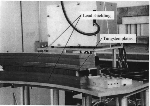
Lead shielding and tungsten alloy anti-scatter plate components of the detector array... 33
The positioning system of a rotary stage mounted on a linear translational stage... 34
D im ensional layout of the CT sensor. ... 35
(a) The aluminum block phantom. (b) Schematic of the aluminum block phantom showing hole dimensions. (c) CT image of the aluminum block phantom... 39
(a) CT image of aluminum cylinder phantom. (b) Edge response function (ERF) for the aluminum cylinder. (c) Line spread function (LSF) for the aluminum cylinder. (d) LSF showing the full width at half-maximum (FWHM)... 40
Theoretical spatial resolution for CT system for various detector (L) and source-object (q) distances, with x-ray spot size and detector width held fixed. ... 41
CT image of aluminum block with interior cavity... 42
(a) The aluminum cylinder phantom with inserts. (b) Schematic of the aluminum cylinder phantom showing the various insert materials. (c) CT image of the aluminum cylinder p h an to m ... 44
(a) CT image of aluminum cylinder phantom showing sections. (b) Computed density vs. position along line AA. (c) Computed density vs. position along line BB. (d) Computed density vs. position along line CC. (e) Computed density vs. position along line DD... 45
Figure 2-16: Figure 2-17: Figure 3-1: Figure 3-2: Figure 3-3: Figure Figure Figure Figure 3-4: 3-5: 3-6: 3-7: Figure 3-8: Figure 3-9: Figure 3-10: Figure 3-11: Figure 3-12: Figure 3-13:
(a) CT image of block phantom reconstructed with 2700 view angles. (b) CT image of block phantom reconstructed with 540 view angles. (c) CT image of block phantom reconstructed with 180 view angles. (d) CT image of block phantom reconstructed with 60 view an g les. ... 4 8 (a) The steel and tin cylinder phantom. (b) Schematic of the steel and tin cylinder phantom. (c) CT image of the steel and tin cylinder phantom using the Co60-based system. (d) CT
image of the steel and tin cylinder phantom using the linac-based system. ... 50
The electric-resistance furnace. ... 53
The clay-graphite crucible inside the stainless steel carriage. ... 53
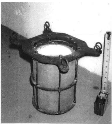
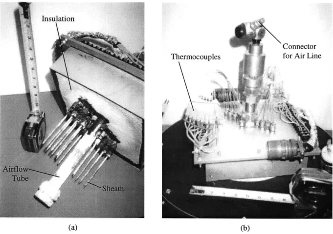
(a) Bottom view of the cooling unit. Note the central airflow tube, the thermocouple sheaths, and the ceramic insulation. (b) Top view of the cooling unit. Note the therm ocou ples...54
Schematic of a vertical cross-section through the solidification platform... 55
Schematic of solidification experiment and CT sensor layout. ... 58
Time-temperature curve for a pure metal. ... 59
(a) CT image of the pure aluminum solidification experiment taken at time = 39.5 minutes. The pixel intensity in the CT image corresponds to the density of the material in units of g/cm3 as represented by the colorbar. (b) Schematic of the CT image features. ... 61
(a) CT image of solidification experiment at time = 39.5 minutes. (b) Plot of computed density vs. position taken along the line shown in (a). ... 62
(a) CT image at time = 22.2 minutes during which the aluminum is entirely liquid. (b) CT image at time = 39.5 minutes during which the aluminum is both liquid and solid. (c) Difference image created by subtracting the CT image in (a) from the CT image in (b). Note that the location of the solidification front is now visible... 64
Difference image of the solidification front position in the pure aluminum at time = 39.5 minutes. The pixel intensity in the CT image corresponds to the difference in density in units of g/cm3 as represented by the colorbar. ... 64
Nine difference images showing the evolution of the solidification front in pure aluminum over a period of 34 minutes, from (a) time=23.3 minutes to (i) time=57.5 minutes. ... 65
Schematic of thermocouple numbering standard... 67
Four difference images at times (a) 23.3 minutes, (b) 28.3 minutes, (c) 39.5 minutes, (d) 57.5 minutes, overlaid with corresponding thermocouple temperature measurements... 69
Figure 3-14: Figure 3-15: Figure 3-16: Figure 3-17: Figure 4-1: Figure 4-2: Figure 4-3: Figure 4-4: Figure 4-5: Figure 4-6: Figure 4-7: Figure 4-8: Figure 4-9: Figure 4-10: Figure 4-11: Figure 4-12: Figure 4-13:
(a) Difference image at time = 28.3 minutes. (b) Computed density vs. position along line shown in (a). (c) Difference image from (a) with noise removed using a Gaussian filter. (d) Computed density vs. position along line shown in (c)... 72 (a) Difference image at time = 39.5 minutes. (b) Computed density vs. position along line shown in (a). (c) Difference image from (a) with noise removed using a Gaussian filter. (d) Computed density vs. position along line shown in (c)... 73 (a) Location of region of interest (ROI) in the CT image. (b) Computed density and temperature in the ROI plotted over the time of the solidification experiment. ... 76 Example of how ring artifacts occur from a compositional variation in object density during d ata acqu isition . ... 7 8 Time-temperature curve for a pure metal and an alloy... 80 (a) Solidification behavior of a pure metal. (b) Solidification behavior of an alloy... 80 Binary phase diagram for aluminum and copper (Mondolfo, 1976). ... 82 Nine difference images showing the evolution of solidification in the hypoeutectic aluminum over a period of 138 minutes, from (a) time=2 minutes to (i) time= 140 minutes.
... 8 4
(a) Location of region of interest (ROI) in the CT image. (b) Computed density and temperature in the ROI plotted over the time of the hypoeutectic solidification experiment.
... 8 5
(a) Location of three ROIs in the CT image. (b) Computed density in each of the three ROIs plotted over the time of the hypoeutectic solidification experiment. ... 86 CT image of the hypoeutectic aluminum at room temperature. ... 90 Photograph of the hypoeutectic aluminum sample sectioned at the same plane as the CT image. The sample has been cut into four pieces for micrograph analysis... 91 Etched sample of the hypoeutectic aluminum. The numbered positions indicate the location where micrographs were taken. ... 91 (a)-(f) Micrographs of the hypoeutectic sample taken at six different positions from the center of the airflow tube ... 92 Density vs. radial position across the hypoeutectic aluminum sample... 93 Hardness vs. radial position across the hypoeutectic aluminum sample. ... 93 Nine difference images showing the evolution of the solidification front in the eutectic aluminum over a period of 70.9 minutes, from (a) time=48.3 minutes to (i) time= 119.2 m in u te s... 9 6
Figure 4-14: Figure 4-15: Figure 4-16: Figure 4-17: Figure 4-18: Figure 4-19: Figure 4-20: Figure 4-21: Figure 4-22: Figure 4-23: Figure 4-24: Figure 4-25: Figure 4-26: Figure 4-27: Figure A-]: Figure A-2: Figure A-3: Figure B-1: Figure B-2:
(a) Location of region of interest (ROI) in the CT image. (b) Computed density and temperature in the ROI plotted over the time of the eutectic solidification experiment... 97 (a) Location of two ROIs in the CT image. (b) Computed density in the two ROIs plotted over the time of the eutectic solidification experiment... 98 CT image of the eutectic aluminum at room temperature. ... 100 Photograph of the eutectic aluminum sample sectioned at the same plane as the CT image. The sample has been cut into four pieces for micrograph analysis. ... 101 Etched sample of the eutectic aluminum. The numbered positions indicate the location w here m icrographs w ere taken... 101 (a)-(f) Micrographs of the eutectic sample taken at six different positions from the center of the airflow tube. ... 102 Density vs. radial position across the eutectic aluminum sample... 103 Hardness vs. radial position across the eutectic aluminum sample. ... 103 Nine difference images showing the evolution of solidification in the 6061 alloy over a period of 106.5 minutes, from (a) time=40.9 minutes to (i) time=147.4 minutes. ... 106
(a) Location of two ROIs in the CT image. (b) Computed density in both of the ROIs plotted over the time of the 6061 alloy solidification experiment. ... 107 CT image of the 6061 aluminum sample. Major voids are marked... 109 Schematic illustrating the different positions a void may have within the x-ray beam... 110 (a)-(d) Four pictures of the 6061 aluminum sample taken at four different slice planes. Each progressive image is approximately 1 mm below the surface of the previous image. M ajor voids are m arked... 111 Comparison of the density evolution curves for the four aluminum solidification exp erim en ts... 114 The x-ray head of the linac mounted in position. Note the cylindrical tungsten collimator at le ft... 12 9
Schematic of the x-ray head collimator design to attenuate the 30' cone beam into a 300 fan b eam ... 12 9 Floorplan of the shielded room designed to house the high-energy CT sensor... 131 Model of heat loss mechanisms for the solidification platform... 134 Schematic of model geometry with dimensions. ... 135
List of Tables
Table 2-1: Measured and computed densities of the various insert materials... 46
Table 3-1: Density of pure aluminum at selected temperatures... 74
Table 3-2: Computed density difference for two difference images... 74
Table 4-1: Results of micrograph analysis on the hypoeutectic aluminum sample... 89
Chapter 1
Introduction
1.1
Background
The casting of liquid metal into a mold to obtain a finished part is one of the oldest and most useful manufacturing processes. It offers tremendous versatility in terms of the size and shape of the final product, allowing complex shapes, internal geometries, or very large dimensions. There are several categories of casting processes, the main division being that of discrete casting versus continuous casting. Discrete casting involves the manufacture of single or multiple near-net-shape parts from either a permanent or expendable mold. Continuous casting differs greatly from discrete casting. It resembles an extrusion or rolling process in that the output of the operation is not a near-net-shape part, but a continuous strand of metal of a chosen cross-section. The primary purpose of continuous casting is the bulk production of metal, such as steel or aluminum, in finite geometries such as billets or slabs for use in secondary manufacturing operations. In all casting operations, continuous or discrete, the driving physical phenomenon is the solidification of the metal from the liquid to solid.
The solidification of molten metal involves complex fluid flow and heat and mass transfer phenomena. Fluid flow during solidification has a large influence on both the crystal structure and homogeneity of the metal casting, as documented by Fisher (1981). Cole (1971) reports that the interactions that take place when a liquid becomes solid may produce structural inhomogeneities of various types. These include dendritic microsegregation, grain boundary segregation, interdendritic precipitation, and porosity at the microscopic level. At the macroscopic level, solidification can affect macrosegregation. With respect to continuous casting, Bobadilla et al. (1993) report that the origins of axial macrosegregation, V-shaped segregates, segregated cracks, and porosity are all linked to the final moments of solidification in a bloom or slab. Cole (1971) asserts that if the defects that accompany solidification can be clearly specified, many of the steps between initial solidification and a final homogeneous product can be reduced.
Currently, computer simulations are used to model the complex solidification behavior in a casting (Chidiac et al., 1993; Lewis and Roberts, 1987; Dalhuijsen and Segal, 1986). However, simulations require precise knowledge of the shape and extent of the solute boundary layer, real growth rate, interface morphology, and nucleation (Curreri and Kaukler, 1996). In addition, interpolations must often be made, always introducing some degree of uncertainty. Lack of adequate thermophysical data, particularly for commercial alloys, is another barrier to accurate modeling. Ultimately, simulations need to be validated, however, current experimental techniques are expensive and fraught with error (Giamei,
1.2
Review of Literature
Because of the crucial role solidification plays in metal casting, a significant amount of scientific and industrial research has been devoted to understanding the solidification process. One large area of study is that of solidification sensors, which aim to experimentally monitor characteristics of the evolving solidification front. This work has produced a variety of different techniques and methodologies.
1.2.1 Direct Measurement Techniques
One of the simplest methods of obtaining information about the solidification front is to mount a tree of thermocouples inside a metal ingot as it solidifies to acquire direct temperature measurements. Bakken and Bergstrom (1986) used this technique in the direct-chill casting of aluminum to determine surface temperature, heat flux, and heat transfer coefficients. These data were later used to verify and improve computer modeling. Although thermocouples placed inside an ingot are an excellent tool, their presence is intrusive to the casting process, which limits their usage. One alternative is to mount thermocouples inside the mold rather than in the metal ingot, as was done for the continuous steel casting process by Ozgu et al. (1985). The temperature measurements were used to calculate time-dependent heat fluxes and heat transfer coefficients for the process which were later incorporated into a two-dimensional solidification model. The major benefit of this technique is that it is non-intrusive. However, the information acquired on the position and evolution of the solidification front is now gathered indirectly, requiring the temperature in the ingot to be extrapolated from the mold temperature data. In general, thermocouple techniques may suffer from slow response time, signal noise, and lack of measurement repeatability.
Story et al. (1993) reported on a liquid core monitoring system for the continuous casting process using segment load measurements. Segment loads, which are greatly influenced by the ferrostatic pressure associated with the presence of a liquid zone, are measured using strain gauges positioned on the segment thickness setting pins. The location of the final solidification point in a cast steel strand is determined by recognizing the transition in segment load between the liquid and solid regions. Schade et al. (1994) documented an increase of 4% in caster line speed through implementation of a liquid core monitoring and control system. It is evident that liquid core monitoring is industrially beneficial. However, it does not yield any significant quantitative information about the shape, position, or movement of the solidification front. In addition, although liquid core monitoring is well suited for continuous casting, it does not transfer well to other types of casting.
1.2.2
Non-Destructive Evaluation Techniques
The benefit of a sensor that does not interfere with the solidification process has fueled the development of many non-destructive evaluation (NDE) techniques. Parker (1983) described a pulsed-echo ultrasonic flaw detector that operates on the principle that longitudinal sound velocity and density are lower in the liquid portion of a casting than in the solid portion. Consequently, the solidification front in a metal casting can be identified because it produces a reflection in the ultrasonic pulse. Laboratory tests using acoustic ultrasound techniques have been attempted on solidification in tin and tin alloys and aluminum and aluminum alloys. Suzuki et al. (1987) reported real-time sensor capability in detecting the solidification front position in tin with a spatial resolution of 10 pm in a 32 mm diameter cylindrical sample. Jen et al. (1997) documented the use of an acoustic ultrasound sensor for monitoring mold filling, gap development, and solidification front movement in aluminum die casting. They encountered problems because casting conditions such as temperature, pressure, melt cleanliness, and mold coating affect the sensor efficiency. As a result, it is difficult to obtain the ultrasonic attenuation in the aluminum part accurately. In addition, once an air gap develops between the aluminum and the mold, the sensor becomes ineffective because the ultrasound cannot be transmitted into the part.
In contrast to acoustic ultrasound, Walter and Telschow (1996) tested a laser ultrasonic sensor to measure the solidification front in tin and tin-lead alloys. A pulsed Nd-YAG laser with a 4 mm spot size generated ultrasonic waves in the liquid metal by ablation. The signal was detected with a confocal interferometer using an argon laser. The system was tested on a moving solidification front in 80 mm of pure tin and Sn-0.6%Pb alloy. Walter and Telschow were able to record the location of the solidification front in both cases, although difficulties were encountered when the solidification front moved faster than 0.1 mm/min. In addition, the presence of a mushy zone scattered the ultrasonic wave and decreased the reflected signal amplitude. Chikama et al. (1996) used a confocal laser microscope combined with an infrared image furnace to study the growth of crystals in iron-carbon alloy melts. The confocal scanning microscope had a resolution of 0.5 Rm and employed a 1.5 mW He-Ne laser. Tests were carried out using Fe-0.83%C and Fe-0.2%C disks having a 4.3 mm diameter and 2 mm thickness. Results in both cases show the planar to cellular and cellular to dendritic crystal transition and cell coarsening.
Kunerth and Wallace (1980) used eddy currents to monitor the solidification in pure lead and Pb-20%Sn samples. An eddy current sensor exploits the conductivity discontinuity between the liquid and solid phases of a metal. Because of this discontinuity, the amplitude and phase of reflected electromagnetic radiation are descriptive of the change in conductivity and the depth at which the change occurs. The extent of solidification in a metal can be determined by continuously monitoring the reflected electromagnetic radiation's amplitude and phase. The results showed that morphological data regarding the solidification front were present in the eddy current measurements. However, the
measurements were subject to errors from thermal gradients present in the mold or melt and segregation effects that altered the conductivity of the metal.
1.2.3
X-Ray Techniques
A subset of non-destructive evaluation techniques involves those sensors that employ and detect x-ray radiation. Fitting et al. (1996) described one such process of locating the boundary in a solidifying metal by measuring the ordered Laue pattern of diffracted x-rays. They used an x-ray tube with a 1.2 mm spot size and a variable x-ray energy that was set at 160 kV for the solidification experiments. The x-rays were measured using a scintillator screen coupled to an image intensifier and CCD camera. To test the apparatus, a 22 mm diameter rod of pure aluminum was melted in a quartz tube furnace and x-ray diffraction measurements were recorded. The results showed an ordered diffraction pattern when the aluminum was in a solid state. As the aluminum neared the melting point, the pattern began to degenerate and eventually resulted in a diffuse ring of scattering when the aluminum was fully melted. In a similar approach, Matsumiya et al. (1987) used synchrotron orbital x-ray radiation to observe solidification in a 300 gm by 10 mm by 50 mm specimen of 3% silicon steel. The x-ray beam was 8 mm in diameter. The Laue spots were observed using an x-ray vidicon camera. Although x-ray diffraction measurements unmistakably differentiate between the solid and liquid states of a metal, the quantitative information regarding the solidification front position, evolution, and characteristics attainable through this technique is limited.
Deryabina and Ripp (1980) reported on the use of x-ray attenuation measurements through a continuously cast steel billet. X-ray radiation was produced using a Cobalt-60 (Co60) radioisotope. The x-rays were detected with a CsI scintillation crystal and photomultiplier. By projecting the x-rays through the steel billet during casting and measuring the transmitted and scattered intensities along a single path, the ratio of the solid phase to the liquid phase in the billet can be determined. This information was used to calculate the shell thickness of the billet at the measurement point and provide feedback to control caster speed to avoid breakout accidents.
A common method of detecting the solidification front evolution in a metal casting is by x-ray radiography. Pool and Koster (1994) used a 160 kV ray source with a spot size of 0.4 mm to acquire x-ray images of the solidification of gallium with a CsI fluoroscopic screen and CCD camera in real time. The 3% density difference between the liquid and solid states was easily visualized. Curreri and Kaukler (1996) performed x-ray radiography studies on the solidification of 1 mm thick samples of aluminum-indium. Using a 100 kV x-ray source with a spot size of 5 jm, the solidification front was visualized with a spatial resolution of 30 jim and a contrast resolution of 2%. Further studies by Kaukler et al. (1997) using the same x-ray sensor showed lead precipitate formation ahead of a moving solidification
front in 1 mm thick Al-1.5%Pb alloy. Using the same radiography apparatus, Sen et al. (1997) documented the solidification front evolution of pure aluminum near 500 tm diameter ZrO2 particles and
500 to 1000 gm diameter voids. X-ray radiography studies such as these provide insight on the evolution and characteristics of solidification. The majority of these techniques operate in real time and yield sub-millimeter spatial resolution with low noise. However, the low photon energy and source strength limits the use of x-ray radiography for metal samples thicker than a few centimeters. This limits the industrial feasibility of an x-ray radiography-based sensor. In addition, techniques such as x-ray radiography produce a single projected view through an object, similar to a medical x-ray. Consequently, there is no depth information about the solidification front.
A natural extension of x-ray radiography is the use of x-ray computed tomography (CT). CT produces two or three-dimensional information on the interior of a solidifying casting. Nagarkar et al. (1993) used an x-ray CT sensor to monitor the melt interface in the production of cadmium telluride crystals. The x-ray source was a 662 keV Cs13 7 radioisotope. The detector system consisted of three 7 mm by 2 mm by 2 mm CdTe scintillators. Nagarkar et al. used this CT system to successfully capture images of the melt interface in the semiconductor crystal with a spatial resolution of 0.7 mm. The 2.5%
to 3% difference between the liquid tellurium and the solid CdTe crystal was readily visible. Chen and Chen (1991) used an x-ray CT system to verify the porosity of the mushy zone in an aqueous ammonium chloride solution. After performing a series of cooling experiments on 30% NH4Cl-H20 solution, CT
scans were carried out on the 10 mm thick mushy zone in the steady-state solution. The density variation across the mushy zone was identified and visual images of the plumes and chimneys were captured.
1.3 Sensor Concept
Although all current sensor technologies provide some degree of information regarding the solidification process, many have some shortcoming. Most of these shortcomings limit the industrial potential of the particular sensor technique in question. Computed tomography, however, offers the possibility of a non-invasive sensor system with the potential of industrial application.
CT-based sensors have been used in non-medical applications since the mid-1980s. The implementation has been mostly limited to defect inspection and dimensional measurement of finished parts, as described by Ross and McQueeney (1990) and Bossi and Georgeson (1992). The feasibility of CT as a method of detecting solidification phenomena was documented in the work of both Nagarkar et al. and Chen and Chen. However, work in this area has thus far been limited to non-metallic materials. Although the solidification studies on semiconductor crystal and aqueous ammonium chloride are
intriguing, the thermophysical and transport properties of these materials differ significantly from those of metals.
A CT sensor for metal solidification is based on the attenuation of x-rays of sufficient energy through the solidifying cast part as well as through any surrounding equipment (Chun et al., 1996). A schematic of this sensor is shown in Figure 1-1. Radiation from an x-ray source is collimated to produce a narrow beam. The beam exits the aperture of the collimator and traverses a path from the source to the detector array. Along this path, the x-ray beam travels through air, the solidified metal shell, the liquid metal core, the solidified metal shell again, and finally through air to the detector. As it travels, the x-ray beam interacts with the material it encounters and is attenuated by the solid and liquid metal. Thus, the incident beam intensity produced at the source will be greater than the transmitted beam intensity at the detector. Since the mass attenuation coefficients of liquid and solid metals are the same while their densities are different (Evans, 1972), the thickness of the liquid and solid phases of the metal that the x-ray beam encounters can be calculated. A complete profile of the density distribution within the strand is mapped by translating and rotating the source and detector about the casting. If the scanning and processing are done rapidly, a real-time, two or three-dimensional image of the solidification front within the casting is generated.
X-Ray Source
1.4
Previous Work
In prior work, a feasibility study was conducted to verify the potential of using CT as a method of detecting the liquid/solid interface in a metal (Hytros, 1996). Because of tin's low melting point, solidification experiments were performed using pure tin contained in a graphite crucible (51 mm ID, 64 mm OD, 152 mm length). The tin was melted by a 500 W cartridge heater inside the crucible and solidified by chilled circulating water around the crucible's exterior. Varying the current to the heater and the flow rate of the water maintained the tin in a partially solidified steady state. The crucible had sixteen chromel-alumel thermocouples mounted inside it. Temperature measurements from the thermocouples monitored the exact position of the solidification front.
The CT system consisted of a 7 mCi Co6 radioisotope as the radiation source and a single Nal scintillation crystal coupled to a photomultiplier as the detector. A Co60 source produces y-ray (identical to x-ray) radiation in two discrete energy bands, 1.16 MeV and 1.33 MeV. In this study, the y-rays from the Co6 source were collimated into a 6 mm diameter pencil beam at the source. The Nal detector was collimated with a 2 mm diameter aperture. The pencil-beam, single detector arrangement necessitated a translate/rotate data acquisition scheme to acquire the proper number of view angles for CT reconstruction. This was accomplished by mounting the solidification experiment on a rotary and translational stage. Figure 1-2 is a schematic of the experimental setup.
Cartridge Heating Unit
K-Type Thermocouple Tree
Graphite Crucible Collimator Shielding Molten Tin Co-60 Source Collimator Data Acquisition 0 & control
0 0 Gamma Ray Detector
Water Cooling Chamber Solid Tin
Rotary Positioning Table Horizontal Positioning Table
Vertical Positioning Table
CT scans of the experiment, in the form of y-ray attenuation data, were acquired once the solidification front of the two-phase tin reached a quasi-steady state. Measurements were recorded at a mid-section through the crucible, in line with the ends of the thermocouples. Figure 1-3 shows a photograph of the experiment. There were 67 transverse measurements (1.9 mm step size) and 60 view angles (3.00 step size). Data were acquired in a photon counting mode, with each measurement acquired over 300 seconds. This resulted in an overall data acquisition time of approximately 14 days.
Figure 1-3: The apparatus for the pure tin solidification experiment.
The CT image was reconstructed using a standard pencil-beam filtered back-projection (FBP) algorithm with a high-cutoff frequency ramp filter. A CT image from the experiment is shown in Figure 1-4. The liquid and solid regions of the pure tin were discernable in the CT image. This density difference is more evident when the pixel values are plotted as a function of position, as shown in Figure 1-4c. Although much noise is present, the image does validate CT as a potential solidification detection tool. However, as witnessed from the image, the spatial and contrast resolutions were poor. In addition, the data acquisition time was unacceptably long. The poor image quality and slow system performance
stem primarily from the choice of x-ray source and detector. The 7 mCi Co6 0 radioisotope did not have a high enough y-ray flux for efficient data acquisition. When coupled with only a single detector, long sample times were required to produce statistically significant data. The long data acquisition time introduced another source of error-fluctuations in solidification front position-which caused a blurring in the CT image.
Obviously, a single detector, radioisotope-based CT sensor is neither practical nor desirable. Despite the limitations, this study found potential in using CT to monitor solidification in metals. Improved CT image quality and decreased data acquisition time could be realized through the use of a high-flux radiation source and a multi-channel data acquisition system.
1.5 Research Goals
The intent of the project at hand is to:
* Develop a high-energy, linear accelerator-based CT sensor system capable of achieving a spatial resolution of 1 mm, a contrast resolution of 1%, and a data acquisition time of 1 second (near real-time). The prototype CT sensor should have the potential for implementation in an industrial environment with only limited modification or revision. * Develop a platform for simulating the solidification conditions of an industrial-size metal
casting.
* Evaluate the capabilities of the CT-based sensor in detecting the evolution of the solidification front in pure aluminum.
" Evaluate the capabilities of the CT-based sensor in detecting the evolution of the solidification front and mushy zone in a variety of aluminum alloys (binary hypoeutectic, binary eutectic, and commercial grade).
" Discuss possible improvements for future development from laboratory prototype to industrial implementation.
As evident from the ongoing research in the field of sensor development, an effective method to non-invasively monitor the solidification front position and evolution during the metal casting process does not exist. CT-based sensors have been examined, but limited work has been done to test their application using metals. In addition, past development has been hampered by the lack of x-ray producing equipment adequate to penetrate large metal castings. This work is the first of its kind to observe the solidification front evolution in large-sized castings of aluminum and aluminum alloy using high-energy CT.
Graphite Crucible Cartridge Heater-,A Steel Bolt Aluminum Cover Liquid Tin Solid Tin (a) (b) (c)
Figure 1-4: (a) Schematic of image features. (b) CT image of solidifying tin and surrounding apparatus. (c) Plot of computed density vs. position taken through a vertical cross-section of the CT image.
1.6 Outline
This chapter provides an introduction to the project, a review of the previous work by others in the field of solidification sensors, and a summary of prior work on a CT-based solidification monitor. The goals of this thesis are also stated. Chapter 2 discusses the prototype sensor design, the principles governing its operation, and its performance characteristics. Chapter 3 covers the design and performance of the laboratory solidification experiment. It also shows and discusses the results of using the CT sensor on solidification where a discrete liquid/solid interface is present. Chapter 4 presents the results and discusses the use of this sensor on metals in which a mushy zone is present. The metals tested include two binary aluminum alloys (Al-l 1.2wt.%Cu and Al-29.7wt.%Cu) and a commercial aluminum alloy (6061). Chapter 5 concludes by summarizing the implications of the current prototype sensor, discussing its application in the casting industry and its potential for scale-up to an industrial environment, and making recommendations for future work. Appendix A provides detailed information regarding the linear accelerator and its operation. Appendix B provides a detailed description of the heat transfer calculations used in predicting the time of the solidification experiment.
Chapter 2
CT Sensor: Principles, Design, and
Performance
2.1
Principles
Computed tomography visualizes a two-dimensional cross-section through the interior of an object at a chosen view-plane, or slice. A three-dimensional image of the object is reconstructed by combining multiple two-dimensional slices. Hounsfield originally developed CT for the field of medicine in the 1970s, where it revolutionized the process of diagnostic imaging with its ability to provide detailed information invasively (Moore, 1990). This ability to investigate the interior of a material non-destructively led to application of CT in industry.
The basic principles of CT are best understood when compared to the technique of radiography, such as the common medical x-ray. Figure 2-1 shows a simple example of the differences in imaging ability between the two methods. In radiography, radiation is directed perpendicular to an object, or phantom, at a single view. The image reproduced represents the total radiation attenuation through the thickness of the object. As a result, any difference between object density and object thickness along a particular path from source to image plane cannot be resolved. In contrast, radiation is directed through a phantom at multiple view angles in CT, as depicted in Figure 2-2. The radiation attenuation at multiple positions is then recorded. Using the attenuation data from these multiple view angles, the local attenuation value for a small volume element within the object is calculated. The local attenuation value is a material-dependent property, independent of object geometry (Evans, 1972). Consequently, the distribution of the local attenuation values reconstructs an image of the interior of the object. The image is representative of a thin slice parallel to the incident radiation beam.
2.1.1 X-Ray Attenuation
Fundamentally, x-ray photons are absorbed or scattered in a single event. Any photons that undergo an interaction are completely removed from an x-ray's path-of-travel. As a result, x-ray photons display exponential attenuation behavior. The probability, P, that a single photon will not undergo one of the three main interactions (photoelectric effect, pair-production, Compton scattering) while traversing through a path length, x, is:
-f pds
Image
Radiography Computed Tomography
Figure 2-1: Comparison of radiography and CT imaging techniques.
Detectors essaammunass Scan Direction Three-Dimensional Object X-Ray Source
Figure 2-2: Schematic of CT imaging technique.
where p is the probability of the particular interaction per unit length. When all three interaction methods are considered, the probability of interaction per unit length is known as the linear attenuation coefficient, yo, defined as:
go = N(T +K +Za) 2.2
where N is the number of atoms per unit volume of the traversed material, r is the probability of photoelectric absorption per atomic cross-section, K is the probability of pair production per atomic section, Z is the material atomic number, and a is the probability of Compton scattering per atomic cross-section. As a result, the number of photons, I, which pass through an object is:
X
I(s)
= Ioe " 2.3where I is the number of photons incident to the object. When calculating x-ray attenuation, the mass attenuation coefficient, y, is more often used. The mass attenuation coefficient is independent of the density and physical state of the material and varies only as a function of photon energy. It is defined as:
p Y= 2.4
P
where p is the density of the material. Substituting Equation 2.4 into Equation 2.3, derives Beer's Law, which is:
X
-fppds
I(s) = Ioe " 2.5
Since both the density and mass attenuation coefficient vary for an object composed of several different materials, Beer's Law is more appropriately written as:
-fJp(s) p(s) ds
I(s) = Ie 0 2.6
2.1.2 CT Reconstruction
In CT, line integrals of the x-ray attenuation measurement over various angles about an object are reconstructed into a planar image of the object. The image plane is divided into two coordinate systems, as shown in Figure 2-3. The first is the object coordinate system (xy), defined in the plane of the object.
The second is the projection coordinate system (z, 9), which describes a set of attenuation measurements through the object. The origin of both coordinate systems is at the center of rotation of the object. As seen in Figure 2-3, the quantity p(z, 6) is a function of both z and 6. Its analytical form is:
p(z,6 )
=
f
, (x, y)c5(x cos 6
+
y sin6
-
z)dxdy
2.7 Equation 2.7 maps the (xy) coordinate system to the (z, 6) coordinate system. This is the Radon transformation (Kak and Slaney, 1987; Cho et al., 1993). The result of the Radon transformation is a two-dimensional function, p(z, 6), or a projection. The set of projects over all 9 constitutes a sinogram. When a CT scan is conducted, the x-ray attenuation measurements form a data set that is, in fact, a sinogram. Projectionp(z,9)
I yy
IntensityIObject
p,0(xy) ) x Intensity I0Figure 2-3: Coordinate systems for CT image reconstruction.
Using the sinogram, it is necessary to solve the inverse of the Radon transform to return information about the object in the (xy) coordinate system. The inverse Radon transform is found by first taking the Fourier transform of Equation 2.7:
P(w,,O) =
fgo(x,y)5(xcose
p
+ ycos&-
z)e'"zzdxdydz=
f go
p (x, y)e-'w (xcosO+"sinO)dXdy= M (w,, ) 2.8
The result of Equation 2.8 is known as the central slice theorem. It states that the one-dimensional Fourier transform of the sinogram is equal to the two-dimensional Fourier transform of the map of the object. The function po(xy) is now obtained by taking the two-dimensional inverse Fourier transform of
M(w,, w,):
g(x, y) = 4Z
f
M(wX,w,)ei " * dwdw,=
472f f
P(wz,6)ewzz|Jdwzd6 2.9where IJ is the Jacobian of the transformation from (w,w,) to (w, 6), and is equal to Iwzl. The Radon transformation is summarized as:
g,(X, y) = F -iP(w,,O ) . jwz\jd 2.10
where F' is a shorthand notation for the inverse Fourier transform. The integration defined by Equation 2.10 is known as a backprojection. A backprojection for the linear attenuation coefficient, y(xy), can be found through five steps (Budinger and Gullberg, 1974):
1. obtain the sinogram, p(z, 6), experimentally
2. obtain P(w, 6) by taking the z-axis Fourier transform of p(z, 6) 3. filter P(w, 6) using a filter-function Iwl
4. obtain the inverse Fourier transform of the result
5. backproject the result.
This process is known as the filtered backprojection (FBP) algorithm. Use of a filter, indicated in step 3, compensates for blurring that results if only a standard backprojection is performed. The inverse of the Radon transform can also be obtained by applying one of several mathematical methods, including summation, series expansion, and analytical solutions. However, in the majority of today's commercial CT scanning and reconstruction equipment, the FBP algorithm is the method of choice because of its
efficient hardware implementation, flexibility, robustness, and model application ability (Schneberk et al.,
1990).
The mass attenuation coefficient of a material is nearly constant for x-rays of high energy, as seen in Figure 2-4 for some selected materials. As a result, once the linear attenuation coefficient is found through solution of the inverse Radon transform, the density distribution through the object follows from Equation 2.4. 10 0 E .0. 0 0 Cz U) 102 L 0 5 10 15
Photon Energy, [MeV]
Figure 2-4: Mass attenuation coefficient as a function of x-ray energy for selected materials.
2.2
Design and Implementation
A typical CT system consists of six components: a radiation source; a radiation detector or detectors; a motion/position system; an operations console; control and processing software; and a test specimen, otherwise know as a phantom (Burstein, 1990). As CT systems developed over time, so did multiple equipment configurations. Although each has its own advantages, successive generations of scanners have improved upon prior shortcomings, primarily by decreasing the data acquisition time. For example, a first-generation system consists of a single radiation source and a single detector. The x-rays are collimated into a thin pencil-beam. This requires both rotation and translation in order to acquire a complete set of attenuation measurements through the object. In a third-generation system, an array of
multiple detectors is used and the x-rays are collimated in a fan-beam configuration, thus eliminating the need for translation in the data acquisition routine. Higher generation systems often involve multiple detector arrays and multiple radiation sources to further decrease data acquisition time.
The CT sensor developed in this work is a modified third-generation rotate-only system.' The radiation source is a 6 MeV x-ray linear accelerator with the x-ray beam collimated into a 300 fan shape. The detector array is composed of scintillation detectors arranged along an arc. To simplify the system design, a position system was chosen to move the phantom within a fixed linac-detector arrangement, rather than rotate the entire linac-detector array in synchrony about a fixed phantom. The positioning system consists of a rotary stage and translational stage mounted in position between the linac x-ray head and the detector array. A custom software application written in C++ controls the system on a PC-compatible computer. The following three sections describe in detail each of the CT system's main equipment components.
2.2.1
Linear Accelerator
The x-ray linear accelerator in the CT sensor is a field-portable MINAC 6 model manufactured by Schonberg Corporation (Santa Clara, CA). The unit can deliver a dose of 300 R/min at 1 m. The linac comprises a standing wave electron linear accelerator (x-ray head), a flexible RF waveguide, an RF head, a power supply/modulator unit, a water circulation unit, and a control console assembly. Figure 2-5 is a schematic of the components. Although the system is field portable, all components were either mounted or fixed in position. Each of the linac components is described in detail in Appendix A.
The x-rays produced by the linac are not monoenergetic. Instead, they range in intensity in a bremsstrahlung spectrum with a maximum of 6 MeV. The average x-ray energy is 1.3 MeV. The spot size is 2 mm. The linac operates in a pulsed-mode, producing x-rays in 5 [ts bursts with a frequency of 180 Hz. The rays are collimated in a 300 cone beam. Additional collimation was added to reduce the x-ray beam to a 300 fan beam configuration. The theoretical beam height at the detectors is 20 mm in size. This corresponds to a theoretical beam height of 10 mm in the center of the CT field. The actual beam height in the center of the CT field was experimentally determined to be 4.5 mm, as discussed in Section
2.3.3.
Although the system is a rotate-only design, in reality data acquisition is performed using both translation and rotation. This is done to increase the effective spatial resolution and is discussed in Sections 2.3.1 and 3.3.
X-Ray Head Control Console RF Waveguide Modulator Umit RF Head
Figure 2-5: Schematic of the linear accelerator components and interconnections.
2.2.2 Detector Array
The data acquisition system consists of an array of 128 detectors, arranged on an arc with a radius of 845 mm, and associated signal acquisition electronics. Analogic Corporation (Peabody, MA) manufactured the basic system; proprietary customizations were done for this CT application. Each detector consists of a cadmium tungstate (CdWO4) scintillation crystal coupled to a semiconductor
photodiode. Each crystal is 20 mm high, 1.8 mm wide, and 3 mm deep, with 1.8 mm space between each detector along the arc. The detectors operate by converting x-ray energy into a proportional amount of visible light. The diodes then convert this light to a current proportional to the deposited energy. The data acquisition electronics (six signal acquisition boards, one timing board, one digital 1/0 board, and one frame grabber board) integrate the current, which then is recorded using custom-developed software on a PC-compatible computer (Jureidini, 1998). The data acquisition electronics are powered using two 5 V and two 15 V power supplies. Figure 2-6 shows the detector array mounted in position.
One shortcoming of a high-energy x-ray CT system is the large amount of scattered radiation that is produced when the primary x-rays interact with an object. When detected, scattered radiation degrades a CT image through blurring and reduced contrast. In the current system, the top and bottom of the array are shielded with a 57 mm thickness and a 45 mm thickness of lead, respectively, to reduce the amount of
scattered x-rays. In addition, tungsten alloy collimator plates, 20 mm high by 1.8 mm wide by 80 mm long, are mounted in front of the array between adjacent detectors. The density of the alloy is 17.5 g/cm3. These "anti-scatter" plates focus the primary x-rays by reducing the scattered x-rays in the plane of the fan-beam. Jureidini (1997) performed a comprehensive study of the scatter reduction of the tungsten alloy plates. Figure 2-7 shows a close-up of the lead shielding and the tungsten alloy anti-scatter plates.
In addition to the 128 detectors located along the array, a set of 64 detectors is positioned directly behind the x-ray head of the linac, out of the primary x-ray beam. The signal measured by these detectors is not attenuated by any intermediary and thus provides an independent measure of the output intensity of the linac during operation. This measure is used to tune the linac to achieve peak performance during a CT scan.
Figure 2-6: The 128 channel CdWO4 detector array. The box behind the array contains
the associated electronics for the data acquisition system. Note the positioning system visible in the lower right of the picture.