Bio-inspired pressure sensing for active yaw control of underwater vehicles

(1)

Bio-inspired Pressure Sensing for Active Yaw

4.8

Control of Underwater Vehicles

by

APR

62 Amy Gao

Submitted to the Department of Mechanical Engineering in partial fulfillment of the requirements for the degree of

Master of Science in Mechanical Engineering at the

MASSACHUSETTS INSTITUTE OF TECHNOLOGY February 2013

@

A u th or ... v ...

Department of Mechanical Engineering December 5, 2012

Certified by... ... . . ...

Michael S. Triantafyllou Professor of Mechanical and Ocean Engineering Thesis Supervisor

Accepted by.

David E. Hardt, Professor of Mechanical Engineering Chairman, Department Committee on Graduate Theses

(2)

(3)

Bio-inspired Pressure Sensing for Active Yaw Control of

Underwater Vehicles

by

Amy Gao

Submitted to the Department of Mechanical Engineering on December 5, 2012, in partial fulfillment of the

requirements for the degree of

Master of Science in Mechanical Engineering

Abstract

A towed underwater vehicle equipped with a bio-inspired artificial lateral line (ALL)

was constructed and tested with the goal of active detection and correction of the vehicle's yaw angle. Preliminary experiments demonstrate that a low number of sensors are sufficient to enable the discrimination between different orientations, and that a basic proportional controller is capable of keeping the vehicle aligned with the direction of flow. We propose that a model based controller could be developed to improve system response. Toward this, we derive a vehicle model based on a first-order

3D Rankine Source Panel Method, which is shown to be competent in estimating the

pressure field in the region of interest during motion at constant angles, and during execution of dynamic maneuvers. To solve the inverse problem of estimating the vehicle orientation given specific pressure measurements, an Unscented Kalman Filter is developed around the model. It is shown to provide a close estimation of the vehicle state using experimentally collected pressure measurements. This demonstrates that an artificial lateral line is a promising technology for dynamically mediating the angle of a body relative to the oncoming flow.

Thesis Supervisor: Michael S. Triantafyllou

(4)

(5)

Acknowledgments

First and foremost I would like to offer my sincerest gratitude to my advisor, Prof. Michael Triantafyllou, who has supported and guided me throughout my thesis while encouraging me to work my own way. With his patience and knowledge, and impres-sive ability to draw ideas together into elaborate and inspiring pictures, he has been a powerful source of both guidance and inspiration. I would also like to thank the number of other professors and research scientists at MIT who have helped me along the way - in particular, Prof. David Trumper for his help in resolving the electrical noise issues within my experiment, and Yuming Liu for his help with the formulation of my panel method simulation.

In my daily work I have been blessed with a friendly and cheerful group of fellow students and labmates. I would like to say a huge thank you especially to members of the Tow Tank Lab, Heather, Jeff, Audrey, James, Steph, and Jacob. The number of stimulating intellectual conversations we had both brightened my days and kept me thinking. Thank you also to Dr. Jason Dahl, who provided valuable advice in the brainstorming phase of this project and experimental design, and to our colleagues over in Singapore, who have offered helpful advice during our meetings.

Finally, I would like to express my love and indebtedness toward my family and my friends. To my dear parents, Tracy and Johnway Gao, thanks for bearing with me through all the happy times and all the hard times, and being a constant source of support and encouragement. I couldn't have done it without you guys! Thanks also for taking me tuna fishing. To my twin brother Allan - my lovable squishy, thanks for always being there for me, for advice, good stories, and good times. To Leah - thanks for always being there to listen and for helping me through many of the most difficult times of the last two years. And last but certainly not least, thanks to my boyfriend Richard, who has often had to bear the brunt of my frustrations against the world and overly long psets, code that won't compile, and experimental anomalies, but who has dealt with me with love and patience. I couldn't have done it without your love and support.

(6)

(7)

List of Figures

1-1 Fish swimming in the ocean and dolphins breaching the water demon-strate the strength and versatility of marine animals (source: National G eographic) . . . . 17

1-2 Left: An underwater cave in the Yucatan Peninsula, Mexico where blind cavefish reside (source: National Geographic). Right: Blind cave-fish in their natural environment (source: OpenCage Photography). . 18 1-3 A photograph of a blind cavefish, overlaid with the approximate

loca-tion of the canal lateral line and neuromasts within it. . . . . 19

1-4 Diagram of flow stimuli sources and the the lateral line system, with enlarged views of the superficial and canal neuromasts [45]. . . . . 20

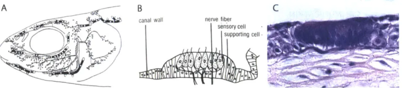
1-5 A - Cephalic lateral line system, displaying both the canal and super-ficial subsystems. B - Diagram of a canal neuromast, highlighting the composing elements. C - Photograph of a canal neuromast, within the canal. (source: Lab of Fish & Shellfish Pathology, Pukyong National

U niversity) . . . . 21

1-6 A sketch shows some capabilities enabled by the lateral line. . . . . . 22

1-7 Left: the hydrocapped biomimetic superficial neuromasts

manufac-tured by McConney et. al. [31]. Right: the SU-8 pillar superficial neuromast constructed by Kottapalli et. al. [28]. . . . . 23 1-8 Left: the LCP and carbon black sensors constructed by Yaul [48].

Cen-ter and Right: Kottapalli et. al's LCP piezoresistive pressure sensors [28]. 23

1-9 An artist's rendition of a submarine equipped with an artificial lat-eral line, exhibiting its ability to detect a school of fish swimming by (source: Chang Liu, University of Illinois). . . . . 26 2-1 Nomenclature used to define the potential flow problem (adapted from

(10)

3-1 A computer-generated rendering of the vehicle constructed for

experi-m ents. . . . . 36 3-2 Analytical solution for pressure field surrounding a Rankine body in

steady uniform oncoming flow. The contours are equal-pressure lines (pressure marked in psi). . . . . 36 3-3 Frontal view and top view of nosecone, depicting the outlines of the

channels cut to bridge the pressure ports and the pressure sensors. All measurements are in inches. . . . . 37

3-4 The towing tank facility in which the experiments were conducted. . . 38 3-5 A diagram of the experimental setup. . . . . 39 3-6 Summary of 33 constant yaw angle experiments, showing a roughly

lin-ear relationship between change in angle and the pressure measured at each port. Error bars show the standard deviation in each experiment

set.. ... ... .. .. ... ... ... . .. . . .. 40

3-7 A proportional gain applied to the differential pressure is shown to

predict the angle of the vehicle with high accuracy. . . . . 42

3-8 A Braitenberg controller aligns the vehicle with the flow following three

large perturbations, which can be seen as variations of the dotted line, the actual angular position. The blue line represents the averaged differential pressure, which the proportional gain is applied to. ... 42

3-9 When a higher gain is applied, it can be seen that the controller

over-shoots zero degrees as it tries to correct the angle following a pertur-bation. The angle experiences decaying oscillations as it settles to zero degrees, but is still stable. . . . . 43

3-10 For an even higher gain, the system is critically stable. The angle never

stabilizes to the desired zero degrees. . . . . 43

3-11 The NMP-like response seen in the sensor output when the vehicle

turns. This results in initial angle correction in the wrong direction with the P controller, which is a cause of delayed response and possible instability. . . . . 44

3-12 The two differential pressures measured over a fast turn from 0 to 16

degrees and back to 0 degrees. The dotted line represents the motion profile. . . . . 44

3-13 The two differential pressures measured over a slow turn from 0 to 16

degrees and back to 0 degrees. The dotted line represents the motion profile. . . . . 45

(11)

4-1 Diagram of the discretized vehicle. The circular vehicle cross-sections are highlighted, and each point represents a corner point. The panels can be visualized as the space between any four points. . . . . 51

4-2 Diagram of the panel-centered frame of reference fixed to a quadrilat-eral constant-strength source element. The corners reflect the trans-formed coordinates of the corners (note that z=0), and P represents a point of interest. (adapted from Low Speed Aerodynamics, [27]. . . . 53

4-3 Left: The velocity potential calculated and plotted over the surface of a 400 panel sphere. Right: comparison between the analytical solution of velocity over the surface of the sphere and that calculated by the panel m ethod. . . . . 57

4-4 Comparison between the surface pressure simulated using the source panel method and the doublet panel method, compared with experi-mentally measured pressures. . . . ... . . . . 58

4-5 Comparison between the surface pressure simulated using the source panel method and the doublet panel method, compared with experi-mentally measured pressures. . . . . 59

4-6 The pressure field over the surface of the vehicle as it turns from 0 to 20 degrees, with the profile of the turn shown in the lower left hand plot. The diagonal lines in the background show the direction of the oncom ing flow . . . . . 61

4-7 Pressure plotted against time and space (panel of the vehicle) for a) static pressure only (no turning), b) a constant velocity turn, c) a slowly accelerating turn, and d) a faster turn. . . . . 62

4-8 Pressure plotted against time and space for the fast turn. a) pres-sure outline for both sides of the vehicle during the turn. b) dynamic pressure outline for both sides of the vehicle during the turn. c) dy-namic pressure measured at only the left sensors. d) dydy-namic pressure measure at only the right sensors. . . . . 63

4-9 Simulated (green) and experimentally measured (blue) pressure ob-served at 4 pressure sensors during a turn from 0 to 16 degrees and back to 0 degrees. Pressure (Pa) is plotted against time (s). The blue arrow represents the direction of oncoming flow. . . . . 64

(12)

5-1 A diagram illustrating the principle of the unscented transformation.

Instead of propagating a single state estimate through a linearized func-tion, a set of sigma points are propagated through the exact nonlinear function . . . . 67 5-2 A comparison between the actual angle the vehicle is at during an

ex-periment, the estimated angle as produced by the Unscented Kalman Filter, and the estimated angle as produced by the proportional esti-m ator. . . . . 71 5-3 A comparison between the actual angle the vehicle is at during an

ex-periment, the estimated angle as produced by the Unscented Kalman Filter, and the estimated angle as produced by the proportional esti-m ator. . . . . 7 1 A-1 Simulated (cyan) and experimentally measured (blue) pressure

ob-served at 4 pressure sensors during a turn from 0 to 16 degrees and back to 0 degrees, with maximum acceleration of 13 deg/s2. Pressure (Pa)

is plotted against time (s). The blue arrow represents the direction of oncom ing flow . . . . . 78 A-2 Simulated (cyan) and experimentally measured (blue) pressure

ob-served at 4 pressure sensors during a turn from 0 to 16 degrees and back to 0 degrees, with maximum acceleration of 46 deg/s 2_{. Pressure (Pa)}

is plotted against time (s). The blue arrow represents the direction of oncom ing flow . . . . . 79 A-3 Simulated (cyan) and experimentally measured (blue) pressure

ob-served at 4 pressure sensors during a turn from 0 to 16 degrees and back to 0 degrees, with maximum acceleration of 65 deg/s 2_{. Pressure (Pa)}

is plotted against time (s). The blue arrow represents the direction of oncom ing flow . . . . . 80

A-4 Simulated (cyan) and experimentally measured (blue) pressure ob-served at 4 pressure sensors during a turn from 0 to 16 degrees and back to 0 degrees, with maximum acceleration of 100 deg/s 2_.

Pres-sure (Pa) is plotted against time (s). The blue arrow represents the direction of oncoming flow. . . . . 81

B-1 Setting the measurement noise covariance to 10x the actual measure-ment noise reduces estimate oscillation, but increases the time delay, as shown in this simulation. . . . . 84

(13)

B-2 Setting the process noise covariance of yaw rate to 1/10th the noise covariance in yaw angle is shown to cause undershoot behavior which follows that in the measurement. This indicates some relationship between allowable unmodeled state change and estimated process noise. 84 B-3 UKF angle estimation produced by a simulated system with 4 sensors. 85

B-4 UKF angle estimation produced by a simulated system with 8 sensors. 85

B-5 UKF angle estimation produced by a simulated system with 18 sensors. 85 B-6 An experimental profile was provided to a simulated system capable of

outputting model-accurate pressure measurements. The result demon-strates the dependence of convergence rate on the estimated measure-ment noise covariance (here, R=70) . . . . 86

B-7 Simulation with an estimated measurement noise covariance of R=20. 86

B-8 Simulation with an estimated measurement noise covariance of R=3. This case demonstrates the accuracy of the UKF state estimate when the measurement noise in the system is negligible. However, for the cases applied to experimental data, the high measurement noise intro-duces more oscillation of the estimate. . . . . 87

(14)

(15)

List of Tables

(16)

(17)

Chapter 1 Introduction

Figure 1-1: Fish swimming in the ocean and dolphins breaching the water demon-strate the strength and versatility of marine animals (source: National Geographic).

Over millions of years, the bodies and brains of fish have evolved in many ways to achieve the objectives which render them capable of survival in the diverse and hostile environments of the oceans, rivers and seas. Extensive study and research have shone light on the incredible grace with which fish are able to maneuver, using their both sensitive and streamlined bodies to exploit the fluid mechanics of the water around them in a way that ocean engineers dream of emulating. A few of the most difficult objectives, which engineers and roboticists have striven to achieve for under-water vehicles and robotic fish in recent years, include station keeping under large perturbations, rapid maneuvering, power-efficient endurance swimming, and trajec-tory planning and tracking [7]. These challenges must be addressed through careful consideration and implementation of sensory capabilities, actuation, and control and planning mechanisms.

While research in actuation has yielded many underwater vehicles that are capable of high speeds and/or fast turns [1,8,19,25], the successful application of these tech-nologies will require faster and more precise underwater sensory systems. Without

(18)

high resolution sensors capable of fast data output, high performance in the obstacle-filled and unpredictable oceanic and littoral enviroments would be near impossible. In recognition of this need, we draw inspiration from nature to develop a new sensing technology based on a fish organ, the lateral line. As sensitive as a human's hearing system and directly integrated with the nervous system, it provides powerful local sensing which equips fish with the reflex-like qualities required for many behaviours, such as escape from predation and schooling. Despite the advantages that it clearly offers marine animals, engineers have yet to develop a technology like this for ap-plication on underwater vehicles. Such a technology could be transformative to the world of underwater robotics, by offering a fast and instinctive way to sense nearby flow structures and obstacles - a sense of touch at a distance. For the realization of such a sensor, much work remains to be done in understanding the nature of the flow in various scenarios, relating these hydrodynamic insights to theoretical pressure measurements, and developing control systems which are capable of utilizing the new knowledge.

Our work here focuses on one scenario and demonstrates the potential of an artifi-cial lateral line within its capacity. In implementing the technology, we study the flow around a basic underwater vehicle, develop simulations which use that understanding to generate expected pressure measurements, and conclude with the development of a control system which uses artificial lateral line feedback to improve performance in the scenario.

1.1 Biological Inspiration: the Blind Cavefish

Figure 1-2: Left: An underwater cave in the Yucatan Peninsula, Mexico where blind cavefish reside (source: National Geographic). Right: Blind cavefish in their natural environment (source: OpenCage Photography).

(19)

The Mexican Blind Cavefish, Astyanax mexicanus, lives in the deep and beautiful underwater caves of Central America (Fig. 1-2), and it is famous for its lack of eyes. Given the mazelike stalagmite and stalagcite formations in the caves, researchers have been drawn to study them, asking the question of "how do these fish survive without eyes?" They found that in the absence of vision, the fish were forced to rely more heavily on their other senses, and as a result, those senses exhibited enhanced sensitivity. In particular, the fish were clearly able to sense the presence of nearby objects by detecting the change in flow surrounding their bodies, using an organ known as the lateral line.

1.1.1 The Lateral Line: Structure and Function

While the blind cavefish best demonstrates the aptitude of the lateral line, all fish possess this sensor in addition to their visual, olfactory, acoustic and tactile sensors. The lateral line consists of tens or even hundreds of hair cell sensors called neuromasts distributed over the body of the fish, and can be divided into two subsystems: the

superficial lateral line system and the canal lateral line system. The superficial lateral

line consists of neuromasts located on the surface of the skin, and detects the velocity of the flow. The canal lateral line system consists of neuromasts within subdermal canals (Fig. 1-3).

Figure 1-3: A photograph of a blind cavefish, overlaid with the approximate location of the canal lateral line and neuromasts within it.

Each neuromast consists of hair cells which are enclosed by a flexible, jellylike cupula, and acts as a mechanoreceptive organ which allows for the sensation of any movement

[14].

While the neuromast is the functional unit of both subsystems, the morphology of the neuromast central to each is very different, in both size and shape

(Fig. 1-4). This is largely due to function. The hundreds of superficial neuromasts on the fish surface interact directly with the flow, and are responsible for deflecting

(20)

as a result of small velocity changes. As a result, they are elongated and act as low pass filters to primarily to detect steady flow.

Superficial neuromast Boundary layer Self-generated flow Canal neuromast Cupula am10 smn Stimulus source -Canal Environmental Cupula pmr=100 flow .___________A____

Figure 1-4: Diagram of flow stimuli sources and the the lateral line system, with enlarged views of the superficial and canal neuromasts [45].

In contrast to this, the neuromasts of the canal subsystem are fewer, larger and flatter. Each neuromast is enclosed within a canal, where there typically exists one neuromast between each set of regularly spaced pores. As water flows across the surface of the fish, pressure gradients are induced between the pores, which these canal neuromasts respond to [13]. As such, they act to detect changes in pressure. These pressure changes result from flow induced by variation of the current, movement of the body, the convergence of an object, or wake structures left by other animals [46]. In contast to the superficial neuromasts, the canal neuromasts are not subject to the boundary layer of the body. As a result, while the fluid inertia within the canals still causes the system to act as a low pass filter, the neuromasts are less affected by the fluid velocity, allowing the system to be sensitive to a range of different stimuli.

In addition, it has been shown that the canals act to tune to specific frequencies of perturbations [41]. Widened canals are most sensitive to lower frequencies (under

60 Hz), such as those produced by movements of crustacean prey. While they tend

to be more sensitive, they also respond more slowly due to the increased fluid inertia within the canals [14].

The canal lateral line system can be further divided into two canals - the trunk canal and the cephalic canal. The trunk canal typically consists of one linear canal which runs laterally down each side of the fish body, while the cephalic canal is more

(21)

B C

Figure 1-5: A - Cephalic lateral line system, displaying both the canal and superficial subsystems. B -Diagram of a canal neuromast, highlighting the composing elements.

C - Photograph of a canal neuromast, within the canal. (source: Lab of Fish & Shellfish Pathology, Pukyong National University)

complex and forms a three-dimensional pattern around the head (Fig. 1-5), which varies between different species of fish. This allows for specialization of the cephalic lateral line to various tasks, such as mating and prey detection [40,41].

1.1.2 Behaviors Aided by the Lateral Line

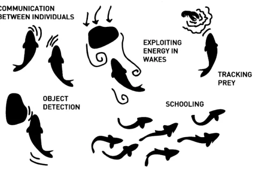
The lateral line has been shown to be fundamental to many fish behaviors, including object detection [11], the localization of moving prey and predators [11,22,41], and environmental mapping [5]. Although these applications are aided by other senses such as vision and smell, the lateral line is crucial to the speed and precision of be-haviors such as the escape response [32]. In addition, in blind fish such as Astyanax

mexicanus, the lateral line is solely responsible for navigation through complex

envi-ronments, response to dangers and prey detection [35,46].

However, while it is easiest to recognize the importance of the lateral line for fish which are blind or are most active at night, this sensor aids in many responses for which other sensors (such as vision) do not provide any feedback. These activities include schooling [38], rheotaxis [34], and analysis of surface waves [3].

Most commonly, to test the influence of the lateral line, behavior is observed before and after anesthetization of the lateral line. With this technique, Coombs et. al. show that the mottled sculpin uses its lateral line to detect the vibration of mechanical dipoles, which were meant to simulate live prey [10]. Schwalbe et. al. used this technique to demonstrate that the peacock cichlid uses its lateral line to detect prey in the dark, thus reducing the competition and danger of feeding during the day [41]. Baker anesthetizes the lateral line in Antarctic fish to determine the responsiveness of the superficial and canal subsystems to various stimuli [2].

(22)

COMMUNICATION BETWEEN INDIVIDUALS

-s

OBJECT DETECTION EXPLOITING ENERGY IN WAKES TRACKING PREY SCHOOLING

p~W,,+qr

Figure 1-6: A sketch shows some capabilities enabled by the lateral line.

image of its surroundings. In order to understand how fish use this sensor to image

its surroundings, it is important to study the nature of the flow field around the fish, and how this field changes as it is subject to different flows and perturbations. By developing a generalized theory surrounding this, it will then be possible to determine how the fish is able to detect the shape of the flow, and decode the patterns to sense the presence of objects, other fish, predators, and prey.

1.2 Relevant Work

1.2.1 Artificial Lateral Line Technology

Toward the creation of an artificial lateral line, several past studies have centered on the development of microelectromechanical systems (MEMS) technology for the creation of an artificial lateral line. The majority of these focus on developing pillar-like mechanical structures which mimic the superficial neuromasts of the lateral line

[15,28,31,47]. In these, a pillar is used to simulate the cupula of the neuromast, and

various types of strain gauges are typically used to measure the deflection of the pillar as it is subjected to different cross-flows. In some, the mechanical pillar is additionally capped with a hydrogel or similar material to simulate the mechanical properties of biological neuromasts. This was shown to significantly decrease the lower threshold

(23)

limit of flow detection and expand the dynamic range of operation due to suppression of background noise [31,39].

Figure 1-7: Left: the hydrocapped biomimetic superficial neuromasts manufactured

by McConney et. al. [31]. Right: the SU-8 pillar superficial neuromast constructed by Kottapalli et. al. [28].

The canal neuromasts have the more general function of detecting pressure, which many commercialized sensors are already capable of doing. As a result of this, a fewer number of studies have aimed to construct sensors which mimic the canal neuromasts of fish. In the ones that do, the majority implement off-the-shelf pressure sensors, which they incorporate into arrays. Hsieh et. al. constructed a sensor array from a high efficiency and low cost piezoelectric material, Polyvinylidene Fluoride (PVDF), which generates an electric potential or electric field in response to applied stress [24].

Kottapalli et. al. developed a MEMS pressure sensor comprised of a liquid crystal polymer (LCP) membrane which encased thin film gold piezoresistors [28]. One study aimed to develop geometrically simplistic and low-cost flexible pressure sensors [48]. These consisted of patterns of conductive carbon black encased in LCP. By detecting the change in resistance of the carbon black as the the sensor deflected, the pressure surrounding the sensor could be deduced.

Figure 1-8: Left: the LCP and carbon black sensors constructed by Yaul [48]. Center and Right: Kottapalli et. al's LCP piezoresistive pressure sensors [28].

(24)

1.2.2 Hydrodynamics of Lateral Line Stimuli

Numerous studies have been performed to study the various stimuli to the lateral line, and the flow structures which are produced by them. It is crucial to develop a strong understanding of these effects in realizing the lateral line technology. While different flows and pressures may be detected by increasingly accurate and sensitive

MEMS pressure sensor arrays, this information possesses very little value without a

methodical way to interpret it. As such, many groups have studied the response of the lateral line to dynamic vibrations, nearby objects, and vortices.

Vibrations are characteristic of nearby prey, and many groups have studied the sensitivity of the lateral line to this stimulus in order to understand its structure and effective range. By far, most studies which are concerned with this use a mechanical dipole oscillating in the range of 50 Hz. to produce the vibrations [6, 9, 12]. These studies have isolated the detection of vibration to the canal lateral line system, and have found that the range of detection is typically about 1.5 times the body length [9].

Another stimuli that has been widely studied is the vortex. Vortices are generated in many scenarios, including in the wake behind a bluff body such as a cylinder, and in the wake of a swimming fish. Fish in the wild often swim in the wake behind objects to save energy (Karman gaiting), and it is thought that the lateral line may help them mediate their position while doing so [29]. Given this, mathematical theories have been formulated to explain how vortices stimulate the canal lateral line [17], and numerous experiments have been conducted to test the effect of vortices passing by real or artificial lateral line systems [16,17,42].

Studies have also been performed to study the role of the lateral line in detection of solid objects. Although it is a passive sensor, the lateral line is capable of detecting the presence of solid, unmoving objects as a fish swims by them. This is due to the flow which is induced by the motion of the fish, which is distorted when objects are present. As such, the lateral line plays an important role in obstacle detection and collision avoidance. Experiments have been performed to study the ability of fish to detect such objects [20, 33], and experiments have also been performed to test the ability of artificial lateral line systems to detect and identify passive objects [30].

1.2.3 Lateral Line Feedback in Algorithm Development

Some groups have attempted to develop algorithms for use with MEMS artificial lateral-line sensors. Pandya et. al. have studied multisensor processing algorithms for underwater dipole localization [37]. Using an artificial lateral line composed of

(25)

hot-wire flow sensors, they developed a minimum mean-squared error (MMSE) estimator in conjunction with hydrodynamic theory based on a general acoustic dipole model. The algorithm was shown to determine the location of a dipole source positioned about 1 cm away with less than 5% error.

Algorithms have also been developed which focus on the localization and charac-terization of vortices and objects

[16,18,30].

The work completed by these researchers typically demonstrate that capability to localize a vortex or object to within 5-10% of its true location. Characterization is typically a harder problem, though Maertens has demonstrated the ability to use an ALL mounted on an underwater foil to localize and determine the approximate size of a cylinder that it passes [30].

No projects known to the author have resulted in the development of full control systems which utilize artificial lateral line technology. All of the work mentioned demonstrates the feasibility of the artificial lateral line, but also highlighted the com-plexity of the inherent hydrodynamics, which must be mathematically defined, for development of appropriate control systems.

1.3 Research Motivation

In light of the previous work accomplished upon this topic, the focus of this project lies not within developing a microelectromechanical systems (MEMS) pressure sensor array for use as an artificial lateral line or in creating new methods of simulating flow and pressure surrounding an underwater body, but rather in applying hydrodynamic theory in developing the control algorithms necessary for using an ALL effectively to navigate underwater.

The majority of AUVs today use sonar and vision for imaging and navigation. However, these sensing systems are limited by blind zones, dark and murky environ-ments, and processing speed. For this reason, they are very powerful when used on large vehicles for the illumination of a global environment, but they face the short-comings of being difficult and time-consuming to intepret, incapable of operating in all environments, and occasionally too slow to sense dangers in time. This, in turn, limits the environments and speeds at which AUVs may operate. In contrast, an artifical lateral line would be constructed from an array of pressure sensors which is small, lightweight, low-cost, and requires extremely low bandwidth and power. A vehicle equipped with an ALL would have the ability to sense its local environment quickly and with high precision, allowing for fast and reflexive responses to dangers or obstacles (Fig. 1-9).

(26)

Figure 1-9: An artist's rendition of a submarine equipped with an artificial lateral line, exhibiting its ability to detect a school of fish swimming by (source: Chang Liu,

University of Illinois).

In particular, an artificial lateral line system concentrated in the frontal region of an AUV could provide important information about incoming obstacles or changing flows. As previously described, the cephalic lateral line system on fish is a com-plex system of canals encircling the head. While the trunk lateral line only pro-vides 2-dimensional information, the morphology of the cephalic system allows for 3-dimensional sensory capabilities which give rise to a diverse range of functions, in-cluding shoaling, prey detection and obstacle avoidance [44]. Given the importance of this system in spatial orientation and movement decisions, we focus solely on de-veloping an artificial cephalic lateral line system in this project, and explore one of

its functions - that of mediating the yaw angle of an underwater vehicle.

Mediating the yaw angle of an underwater vehicle is a useful function, as it allows for the vehicle to travel with the current instead of at an angle, reducing energy loss due to crossflows and minimizing control effort that would be used in fighting the strong munk moment that arises from traveling at angles. Furthermore, traveling with the current results in less drift and therefore less uncertainty in the vehicle position over time. Yaw angle detection can also serve as an additional feedback mechanism for state estimation, aiding in the task of vehicle localization.

The overarching goal of our work here is to develop a theoretical basis for un-derstanding the surface pressure that results from different flows over the body of an underwater vehicle. With such an understanding, we can work toward the

de-AUV

Ar tificial La te ralI Line

(27)

velopment and implementation of control algorithms which are capable of using the feedback from an ALL effectively to detect and control a vehicle's orientation relative to a current. By showing that a small number of pressure sensors can be used to accurately detect the angle and used as feedback to return the vehicle to zero degrees relative to the flow, we provide a proof of concept that this technology can serve as a low-bandwidth sensor for a simple application. In addition, this project provides a framework for more complex applications, such as the control of an underwater vehicle in turbulent flow or in the wake of an object. In summary, it brings us one step closer to equipping modern-AUV's with a mechanosensory underwater system which would be able to sense and utilize underwater flows and currents in a similar fashion to fish in nature.

1.4 Chapter Preview

In Chapter 2, the basic governing equations for this problem are presented, from a fluid dynamics perspective. Potential flow theory is introduced, and we comment on its qualities which make it an ideal modeling tool for this application. The concept of using elementary solutions to Laplace's equation as elements of a solid body is introduced, and the governing equations derived.

In Chapter 3, the experimental test setup and underwater vehicle are described. Several brief notes are included on the shape of the vehicle, and designing for reduc-tion of mechanical and electrical noise. The experiments conducted are summarized and their most relevant results are presented. These include a set of static towing ex-periments, experiments conducted with a basic proportional controller implemented, and experiments conducted to test the dynamic response of the vehicle. Regarding the last, added mass effects are discussed, and their relevance to the problem is ana-lyzed. Finally, the concept of a model based controller is introduced to address the issues brought up.

In Chapter 4, we develop the first component of a model-based controller: the model. Various computational fluid dynamics approaches are compared, and we mo-tivate the choice of a panel method for modeling the vehicle. A 3D Rankine source

panel method is chosen and developed. The boundary value problem is described,

and we discuss how the panel method is used to solve the problem. Results from the final model are presented for simulations conducted at static yaw angles, and for dynamic maneuvers. For both, the simulated results are compared with previously collected experimental data, and there is good correlation.

(28)

In Chapter 5, we develop the second component of a model-based controller: the observer. Some background on state estimation and Kalman Filtering is first pre-sented, followed by an introduction to the Unscented Kalman Filter. We describe how the UKF is used to predict the states of the vehicle, and discuss the key param-eters. A few results from implementation of the UKF are presented, and are shown to produce much improved estimates, compared with the controller which operated on an estimate generated from comparisons against static pressure measurements.

Finally, in Chapters 6 and 7, the project is summarized and conclusions drawn, and a few recommendations for future work are provided.

(29)

Chapter 2 Hydrodynamic Background

This chapter will provide an overview of the general hydrodynamic theory which describes the flow around a 3D body.

2.1 Governing Equations

Within the fluid, we have conservation of mass:

(PO1 dV = 0

Which simplifies when we assume the fluid is incompressible:

V -V= 0

Conservation of momentum can be written:

(2.1)

(2.2)

pD = p

Dt 8 t + - vi = F + V- T

Where T represents the stress tensor. This can be easily rewritten as Navier-Stokes equation:

p

Ot7

a

+-V = -Vp+ pV2u+f (2.4)

In our case, viscosity is neglected, an assumption which will be justified at a later point. Setting viscosity to zero and rewriting the first term using the velocity

poten-(2.3) OP+

(30)

-tial, equation (2.4) becomes:

P(at + V = -Vp + f (2.5)

2.2 Modeling Pressure within the Fluid

The primary variable of interest is pressure, which is defined by Bernoulli's unsteady pressure law. This can be derived from equation (2.5) by expanding the second term on the left hand side and replacing the force vector f with gravitational force. The cross product of the velocity and vorticity is:

i6

xx Vx 6 (2.6)

V

6-VV--V

(2-6

(2.7)

For a potential flow, vorticity is zero, and so the left hand side of equation (2.6) is zero. Substituting the result into equation (2.5) and integrating out all the spacial derivatives, this yields Bernoulli's Unsteady Pressure law:

P - (0 1 72+gz (2.8)

Where p is the water density,

#

is the velocity potential at the point of interest, g is the gravitational acceleration constant, and z is the current water depth. It is important to note that this is defined in the inertial frame of reference, and when we are concerned with the pressure at a material point (e.g. a point on the surface of a moving body), the equation must be rewritten to account for the material derivative:

P = -p

(Dt

Do V# + 1|V#|2+gz (2.9)

u ± ₂Iw Fz

To solve, we must first analytically define $.

2.3 Potential Flow

In hydrodynamics, potential flow describes the velocity field as the gradient of a scalar function.

(31)

This allows for clear and analytical functions to be derived which represent various flows. Potential flow is limited to applications in which vorticity and turbulence are minimal, because the flow is assumed to be inviscid, incompressible and irrotational. As a result, it is best applied in high Reynolds number regimes, but when applied properly is capable of estimating the flow around complex geometries with high accu-racy. For simulation of complex geometries, the elementary solutions of the potential flow problem may be distributed in a manner that satisfies the appropriate boundary

conditions.

The mathematical problem can be illustrated by Figure 2-1. Here, we have

rep-Saw

Figure 2-1: Nomenclature used to define the potential flow problem (adapted from Low Speed Aerodynamics [27]).

resented an arbitrary volume of fluid V in which we wish to solve for the flow char-acteristics. A body SB within the fluid posesses a wake Sw. A designated point of interest is P, and the normal vector h' is defined to point outside of the region of interest. Where G is Green's function (the potential of a source) and

#

represents the potential of the flow of interest (both scalar functions of position), the divergence theorem gives:

J(GV# - #VG) -&dS =

f

(GV2₀

- OV 2G)dV = 0 (2.11)

In the case where P is outside of the fluid volume of interest, both G and # satisfy Laplace's equation, so the right hand side of the equation goes to zero. To extract P from V, we enclose it in a small circle of radius e. Rewriting equation 2.6, this yields:

(GV# - #VG) -ndS (2.12)

(32)

Substituting in the definition of Green's function, G = 1/r, and expanding:

J dS (r r jV- r dS = 0 (2.13) spheree c ( 1 y + 2

Integration around the surface of the sphere gives fSphere dS = 47e2, and assuming

&q#/Or ~ 0 because

4

is likely a well-behaved function that will not vary much in the tiny sphere, the first term becomes:

- +

)

dS = - dS = -4,r#(P) (2.14) Finally, we substitute this back into equation 2.8 for a formula that provides the velocity potential at any point P, given the values of

#

and O#/On on the boundary

S:

#(P) = j

V#~

- #V V -dS _(2.15) 47r

- 47

_fs

r _r)

As a result, the problem is now reduced to finding these values on the boundary. As previously stated, to solve for the flow surrounding a complex shape, elementary solutions are distributed in a manner that satisfies the appropriate boundary condi-tions. The elementary solutions most commonly used in this context are the doublet (p) and source(o-), where a doublet embodies the difference in potential between the inside and outside of a boundary, and a source represents the difference between the normal derivative of the inside and outside potentials:

P = -(# - #1) (2.16)

- (00-001(2.17)

On On

The potential at point P can now be rewritten in terms of these elementary solutions:

$(P) = -[,(1 - p o- (1)] dS +#Ow + #00(P) (2.18)

4 s r On r_

#w

denotes the potential of a wake, in the case that the user wishes to define it for increased accuracy, and

#,,(P)

denotes a constant potential in the region, which may be added for specific scenarios such as moving reference frames. This is the general form for the potential at a point P within a volume of interest, provided a known distribution of sources and/or dipoles over the surface of any bodies present within

(33)

the volume.

2.4 Superposition Principle

Up to this point, it has been implied that the total potential at any point can be found by summing individual contributions, or integrating over a contributing surface. This

principle of superposition can be proven through the following example. If:

VrI = and Vr2 = (by definition) (2.19)

Dr Dr

then Vrl + Vr2 = + (2.20)

Dr

or

provided the boundary conditions are linear, which is the case for rigid non-moving

walls or infinite space. Equivalently, if we let# =

#1

+

#2,

r (1 + 2) = 1+ 02 (2.21)

Or

Dr

Or

This linear property means that if the velocity potential is known for two different

flows, then the sum of the two flows will also be a solution to Laplace's equation.

This indicates that a complex flow can be formulated by summing any number of elementary solutions.

While this concept seems straightforward, it is this idea which makes potential flow theory so powerful, because it allows for the formulation of complex 3-dimensional flow problems as linear problems. This eliminates the need to solve the governing differential equations for each fluid element, which would be a lengthy and computa-tionally taxing process. Therefore, if a flow problem can be modeled using potential

theory, finding its solution becomes a far faster and more manageable process.

2.5 Application Within This Project

Within this project, the problem description involves a 3D body which moves through a fluid volume, translating and rotating over time. We aim to calculate the potential on the surface of the body, provided the state of the vehicle (position and velocity of each point). Given the potential, the surface velocity and surface pressure can then be obtained. To solve for these parameters, we require a discretization of the body geometry, definition of source and/or dipole locations and strengths over the body. Panel methods are a well-studied approach for this type of problem, and its

(34)

(35)

Chapter 3 Testbed Construction and

Experiments

A testbed was constructed to investigate the feasibility of using an artificial lateral line

system for yaw angle feedback within a control system. The setup allows for testing to occur in a more controlled environment, where parameters such as flow speed and angle can be precisely dictated, and the dynamics of a vehicle with thrusters and control fins does not have to be considered. To address the goal of estimating and correcting a vehicle's angle of attack, sensors mounted on the experimental vehicle act as a simplistic replica of the fish's cranial lateral line system. This subsystem was chosen as the focus because its location imparts upon it exceptional sensitivity to pressure fluctuations resultant of changes in orientation.

3.1 Vehicle Design

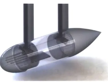
The setup consists of a towed underwater vehicle (measuring 0.7 m long by 0.15 m diameter) with five off-the-shelf pressure sensors (Freescale MPXV7007) mounted at the head (Fig. 3-1). The MPXV7007 sensors are monolithic silicon piezoresistive transducers in a thermoplastic (PPS) surface mount package. They feature a range of -7 to 7 kPa and 5% maximum error over 0' to 85'C, and are internally amplified to output a signal between 0.5 and 4.5 V. The analog signals are read by an NI

USB-6009 data acquisition unit, and processed using code written in LabVIEW (National

Instruments, Austin, TX).

The shape of the vehicle was chosen such that the nosecone resembles a 3D Rankine body, for which an analytical solution to the flow disturbance within a steady uniform oncoming stream is readily available (Fig. 3-2). The pressure ports are chosen to be

(36)

Figure 3-1: A computer-generated rendering of the vehicle constructed for experi-ments. 3-2 1 0 -1 -2 -3 -2 0 2 4 Distance (in) 0.76 0.74 0.72 0.7 0.68 0.66

Figure 3-2: Analytical solution steady uniform oncoming flow. marked in psi).

for pressure field surrounding a Rankine body in The contours are equal-pressure lines (pressure

laterally spaced 0.88 inches apart. Interior channels within the nosecone act to bridge the pressure ports to the sensors mounted within the body. In this way, the sensors are not directly exposed to water (MPXV7007 sensors are not compatible with water). In addition, this structure is easier to construct, because it eliminates the need to mount the sensors to the inside of the curved nosecone. Due to manufacturing constraints,

(37)

the channels were constructed to be wider near the inside and narrower at the surface. Calculations were performed to ensure that the narrow region was sufficiently long to prevent water from entering the wide channel. A drawing of the nosecone architecture is presented in Figure 3-3.

.750

--1.874

Figure 3-3: Frontal view and top view of nosecone, depicting the outlines of the channels cut to bridge the pressure ports and the pressure sensors. All measurements are in inches.

The tail section tapers to a point, streamlining the vehicle. This acts to reduce flow separation. While separation would likely not affect pressure measurements at the front of the vehicle, reducing separation acts to reduce oscillatory body forces which would result in greater mechanical vibration.

Both the nosecone and tail section were manufactured by CNC lathe from high density polyethylene (HDPE). The material provided a smooth finish when turned with a high speed steel (HSS) cutting tool. The main body, or pressure vessel, is constructed from a 0.25 inch thick acrylic tube, sealed at both ends with Buna-N 0-rings inserted into rectangular grooves cut into the nosecone and tail section. Two steel shafts are allowed to rotate in bushings, and the supporting rods are directly threaded into them. The rotation allows for pitching maneuvers of the vehicle, which

were unexplored within this project but could be a direction for future work.

3.2 Experimental Setup

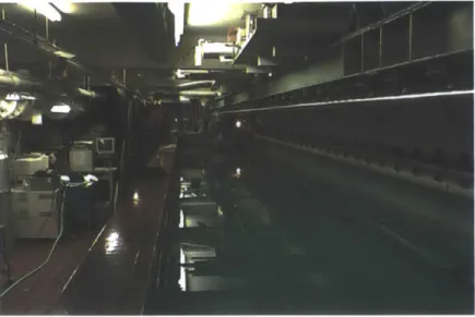
The experiments were carried out in the MIT Towing Tank, a 33 m long pool that is approximately 2.6 m wide and 1.2 m deep (Fig. 3-4). The testbed is mounted to a carriage which is driven down the length of the tank by a simple drive system.

(38)

Figure 3-4: The towing tank facility in which the experiments were conducted.

To produce carriage motion, a Compumotor brushless DC servomotor drives a pulley system. The vehicle is mounted to the carriage via two steel rods, which are enclosed in streamlined aluminum tubing struts to minimize mechanical vibrations that would occur as the result of separation of the flow surrounding the rods. The carriage is towed at a fixed rate of 1 m/s for all experiments. A Copley STA2510 direct drive motor mounted to the carriage actuates the vehicle in yaw, to achieve or maintain various angles of attack. A position sensor within the motor allows for angular po-sition feedback. A computer and other supporting hardware are also located on the carriage for vehicle control and data processing (Fig. 3-5). Pressure measurements were logged at a sampling rate of 1000 Hz.

3.3 Reduction of Noise in Experiments

Mechanical and electrical noise were nontrivial problems within this project. Several measures were taken to reduce each.

Mechanical noise was reduced by mounting the vehicle with two struts as opposed to one. Above the motor, a triangular strut mounts the assembly to the carriage, which further stabilizes the system. Within the vehicle, vibration of tubes can cause fluctuations in the measurements, and this was reduced by drilling channels directly into the nosecone, and connecting them to the sensors with extremely short tubes. Additionally, the vehicle was streamlined to reduce separation and vortex-induced vibrations (VIV), and the supporting rods were surrounded by streamlined tubing which rotated with the flow. This acted to reduce VIV from the supporting rods.

(39)

Figure 3-5: A diagram of the experimental setup.

Even with these precautions, some mechanical vibrations were still present. It could be possible to further reduce the vibrations by adding a third supporting rod to the assembly.

A large amount of electrical noise was present when the yawing motor was switched

on. As the STA2510 is a powerful direct-drive motor, it is likely that it produces a large amount of electromagnetic interference. To reduce this, the motor drive was grounded to the metal carriage, and separate power supplies were used to power the sensors and the motor hardware. Shielded wires were used to transmit the sensor signals, and RC filters were installed between the cables and the DAQ to filter out high frequency noise. Furthermore, as the motor drive unit is powered through the wall outlet, there may be increased noise from the AC signal. To reduce this, an isolation transformer was placed between the wall outlet and units it supplied (motor drive, power supply).

3.4 Preliminary Experiments

The preliminary tests consisted of 33 constant yaw angle experiments - 3 tests each

at two degree intervals between 0 and 20 degrees, in order to observe the relationship between yaw angle and pressure at the five sensor locations. These experiments

(40)

demonstrated the existence of a strong relationship between the angle of the vehicle and the pressure difference between the left and right sides of the vehicle (hereby referred to as the differential pressure). Averaged results from these experiments are presented in Figure 3-6. In this figure, the relationship between angle and pressure

600 _Sensor Location: 400 -Left 2 i :- -Left 1 200 -Center -Right 1 U)0 _0- -Right 2 -200 -400 -0 5 10 15 20 Angle (degrees)

Figure 3-6: Summary of 33 constant yaw angle experiments, showing a roughly linear relationship between change in angle and the pressure measured at each port. Error

bars show the standard deviation in each experiment set.

is roughly linear for all five ports. The data is very consistent within experiment sets, with an average standard deviation of 10.48 Pa for an average angle standard deviation of 0.13 degrees per experiment set (hard to align the vehicle at specific angles - there is some mechanical error which is recorded). The standard deviation for small angles is somewhat higher, possibly because the the relative angle deviation is higher, and for small angles the pressure is more sensitive to slight changes in angle. There is a small discrepancy in the data for the second sensor on the right. This is likely due to mechanical error. Due to the fast starts and stops of the carriage during experiments, some water may have entered the concerned channel. This would result in an increased pressure baseline, as the air in the channel cannot escape, and would be more compressed. Since the preliminary experiments were not intended to inform a control system, the experiments were not repeated.

The linear relationship between angle and pressure suggested that a Braitenberg type controller [4] might be able to regulate the angle of the vehicle by simply apply-ing a proportional gain to the differential pressure observed. Braitenberg controllers were a concept introduced by Valentino Braitenberg in 1984 as a simple way to rep-resent behavior based artificial intelligence. The premise is that a vehicle may posess a number of primitive sensors which are directly connected to effectors, such that a sensed signal immediately produces a particular motion. Depending on the architec-ture of the sensor-effector connections, the vehicle can be made to seem intelligent,

(41)

striving to achieve certain scenarios and avoid others. This type of controller ap-peared intuitively relevant to this problem, because it is easy to imagine that our vehicle might want to turn away from, or toward, higher pressure on one side. In the case of correcting an angle of attack, the vehicle would generally turn toward higher pressure, in order to minimize the pressure differential between its sides. Additional functions applied to the sensor outputs can create even more complex behaviors. For instance, a proportional controller applied to the pressure differential can create a smooth range of motion.

3.5 Basic Controller Implementation

A second set of experiments was conducted to test this concept. A proportional

controller was developed in LabVIEW and implemented on the system, with the goal of returning the vehicle to zero degrees following any perturbations and maintaining that orientation. First, to determine an appropriate gain for the controller, a test was conducted in which the vehicle was sinusoidally yawed between -20 and +20 degrees, and the average pressure differential between the left and right sensors was recorded. The required gain was calcuated by dividing the average differential pressure by the angle, and was found to be 16877 Pa/deg. By dividing the recorded differential pressure by this gain, it was found that the angle of attack could be recovered with high accuracy over the entire angle range (Fig. 3-7). The gain is likely to be highly dependent on oncoming flow velocity, so for different towing velocities, it would need to be adjusted. However, for small deviations, and for the altered apparent velocity

at each port due to yawing and pitching, using a constant gain may be sufficient. Implementing the Braitenberg controller with proportional gain, the vehicle was found to accomplish the goal of returning to zero degrees following perturbations (Fig. 3-8), but with a varying time lag. Furthermore, at higher gains, the system became unstable (Fig. 3-9, 3-10). This demonstrated the shortcomings of the Brait-enberg controller, and suggested that a more complex, model-based controller would be required for improved system response.

3.6 Dynamic Response

To investigate the pressure fluctuation during dynamic maneuvers, a final set of ex-periments was conducted in which the vehicle was commanded to turn sharply from 0 to 20 degrees while being towed forward at 1 m/s. The differential pressure measured

(42)

10 15 20 25 Time (s)

Figure 3-7: A proportional gain applied to the differential pressure is shown to predict the angle of the vehicle with high accuracy.

a) cJ) a) U) 200 205 210 215 220 Time (s) 225

Figure 3-8: A Braitenberg controller aligns the vehicle with the flow following three large perturbations, which can be seen as variations of the dotted line, the actual angular position. The blue line represents the averaged differential pressure, which the proportional gain is applied to.

in one experiment is shown in Fig. 3-11. Here, we have focused in on the turning region so that the response can be clearly seen. These experiments revealed that when the vehicle turned from one static angle to another, the differential pressure re-sponse exhibited initial undershoot, a characteristic often seen in non-minimum phase

Bio-inspired pressure sensing for active yaw control of underwater vehicles

Bio-inspired Pressure Sensing for Active Yaw

Control of Underwater Vehicles

by

APR

62

Amy Gao

@

Bio-inspired Pressure Sensing for Active Yaw Control of

Underwater Vehicles

by

Amy Gao

Abstract

Acknowledgments

Contents

List of Figures

List of Tables

Chapter 1

Introduction

1.1

Biological Inspiration: the Blind Cavefish

1.1.1

The Lateral Line: Structure and Function

[14].

1.1.2

Behaviors Aided by the Lateral Line

-s

p~W,,+qr

1.2

Relevant Work

1.2.1

Artificial Lateral Line Technology

1.2.2

Hydrodynamics of Lateral Line Stimuli

1.2.3

Lateral Line Feedback in Algorithm Development

[16,18,30].

1.3

Research Motivation

1.4

Chapter Preview

Chapter 2

Hydrodynamic Background

2.1

Governing Equations

p

a

2.2

Modeling Pressure within the Fluid

(2-6

#

(Dt

2.3

Potential Flow

#

f

4

)

#

V#~

fs

#w

#,,(P)

2.4

Superposition Principle

or

#1

#2,

Or

Or

Or

2.5

Application Within This Project

Chapter 3

Testbed Construction and

Experiments

3.1

Vehicle Design

3.2

Experimental Setup

_fs