Design rules and models for the synthesis and optimization of cylindrical flexures

Design Rules and Models for the Synthesis and Optimization of

Cylindrical Flexures

by Maria J. Telleria S.M. Mechanical Engineering

Massachusetts Institute of Technology, 2010 S.B. Mechanical Engineering

Massachusetts Institute of Technology, 2008

SUBMITTED TO THE DEPARTMENT OF MECHANICAL ENGINEERING IN PARTIAL FULFILLMENT OF THE REQUIREMENTS FOR THE DEGREE OF

DOCTOR OF PHILOSOPHY IN MECHANICAL ENGINEERING AT THE

MASSACHUSETTS INSTITUTE OF TECHNOLOGY JUNE 2013

 2013 Massachusetts Institute of Technology All rights reserved.

Signature of Author……… Department of Mechanical Engineering May 10th, 2013

Certified by……… Martin L. Culpepper IV Associate Professor of Mechanical Engineering

Thesis Supervisor

Accepted by……...……… David E. Hardt Professor of Mechanical Engineering Graduate Officer

Design Rules and Models for the Synthesis and Optimization of Cylindrical Flexures by

Maria J. Telleria

Submitted to the Department of Mechanical Engineering on May 10th, 2013 in Partial Fulfillment of the Requirements for the Degree of Doctor of Philosophy in

Mechanical Engineering

ABSTRACT

Cylindrical flexures (CFs) are defined as systems composed of flexural elements whose length is defined by the product of their radius of curvature, R, and sweep angle, ϕ. CFs may be constructed out of a cylindrical stock which leads to geometry, manufacturability, and compatibility advantages over planar flexures. However, CFs present a challenge because their mechanics differ from those of straight beams, and although the modeling of curved beams has been researched in detail [1–4], it has yet to be distilled into compliant element and system creation rules. The lack of relevant design rules has inhibited the process of concept generation and optimization of CF systems, preventing these systems from becoming pervasive in engineering applications. The design guidelines and models developed in this work enable (i) the rapid generation of multiple concepts, (ii) the efficient analysis of different designs and selection of the best design, and (iii) the effective optimization of the chosen concept.

The CF synthesis approach presented in this thesis has three components: (i) analysis of element mechanics models to reveal key parameters, (ii) understanding of how the key parameters affect the flexure performance and (iii) guidelines as to how to assemble and optimize CF systems. With the knowledge generated designers will be able to rapidly layout possible designs using the element building blocks and system creation rules, and then use the identified key parameters to optimize a design. The synthesis guidelines were established and tested through the development of two case study flexures: a CF linear guide and an x-y-θz stage. The case studies demonstrate the increased design space of CF systems, which makes it possible for these new flexure mechanisms to meet functional requirements that could not be met using traditional straight-beam flexures.

Thesis Supervisor: Martin L. Culpepper

A

CKNOWLEDGEMENTS

I am extremely grateful for Prof. Culpepper’s guidance, support, and encouragement. From the first time I worked in his lab as a UROP he encouraged me to pursue research and later on graduate school. I cannot say thank you enough for the 5 years that he has served as my advisor. His advice and encouragement were instrumental in my application for the National Science Foundation Graduate Fellowship. The NSF fellowship made it possible for me to pursue my work in Cylindrical Flexures. I am extremely grateful for NSF’s support in my education and sincerely hope that the fellowship continues promoting the advancement of new fields.

Prof. Sangbae Kim and Dr. Mark Schattenburg graciously accepted to join my committee, and I am sincerely grateful for their valuable time, advice, and questions. Every committee meeting was stimulating, and I always walked away with exciting questions and ideas. My entire committee constantly probed at my progress, and insisted that I consider new avenues of thinking during my investigation. I was also extremely fortunate to have Prof. Evelyn Wang as a mentor. Our numerous lunch meetings were always refreshing and uplifting.

Further, I am sincerely thankful to all of my present and past colleagues at the Precision Compliant Systems Lab. Regardless of their immense workloads, they were always ready and eager to help: whether it was a lively discussion of instrumentation or lending an extra hand when one was needed. In particular, I would like to thank Robert Panas, Jon Hopkins, and Chris DiBiasio for their help and friendship.

Throughout my time in graduate school I had the wonderful opportunity of working with several undergraduate students (UROPs). I am thankful for the time and effort that each of my UROPs invested in their projects. I have enjoyed serving as their mentor and have learned a considerable amount from our time in research. I am especially grateful to Laura Matloff who worked with me on Cylindrical Flexures and who was the first guinea pig for the models and rules that I developed. Laura always impressed me with how quickly she picked up the new material and how she always asked the right question. I am also extremely thankful to have Julie Wang work with me on the SQUIShbot project. For two years, she has been instrumental in the project’s development through her work on ER valves. During these two years I have gotten to

see Julie grow as an engineer, she has expanded her understanding of fluids, electronics, design, and manufacturing with ease.

During my graduate career I had the privilege of working with the MIT SQUIShbot team on creating cm-scale, low-cost robotics. Working with this group of students, professors, and Boston Dynamics engineers has been a highlight of my years at MIT. The project was and continues to be extremely challenging but I’m continually amazed by the strides the team has achieved. Led by Prof. Hosoi, Prof. McKinley, Prof. Culpepper, Dr. Iagnemma and the work of numerous students, this team was able to produce multiple cm-scale robots. I am very thankful for the guidance and advice I received from all of the professors and engineers. It was a pleasure to work alongside students like Nadia Cheng and Ahmed Helal whose work I admire and whose friendship I value even more.

This work would not have been possible without Prof. Hunter’s BioInstrumentation lab or the machine shop in building 35. The CF linear guides created for this thesis were machined in the BioInstrumentation Lab with the help of Jean Chang, Ashin Modak, and Adam Wahab. I would not have been able to make these prototypes without their assistance and patience. Similarly, the staff in the shop has been so helpful throughout my entire time at MIT, from helping me make my undergraduate thesis to giving me advice on how to manufacture the CF systems. Pat, Dave, and Bill make it possible for all students to excel in their research. Their help and experience has been essential for countless theses, and I will always value their friendship.

My experiences in the laboratory of manufacturing and productivity, LMP, have been a highlight of my studies at MIT. The students and the faculty in LMP are truly amazing colleagues and friends. I cannot imagine a graduate career without the lively and supportive environment that LMP promotes. There are countless friends that deserve thanks for their support, and for simply listening and being available. In the final push to graduate, I am so grateful to have had Melinda, Bob, Maia, Caitlin, and many others working in our shared office. I always looked forward to returning lab and seeing them; they are the reason I never wanted to work from home. This sentiment extends to the mechanical engineering department. I can think

necessary love and support regardless of the situation. They were the ones who had to deal with my endless questions as a child and who encouraged me to pursue engineering. Los quiero muchisimo y muchas gracias por todo. I would also like to thank Asiri for his love and support. There have been many days when taking a shortcut was too tempting and yet he always knew how to encourage and help me so that I always did my best. To Joy Johnson and Monica Orta I would like to say thanks for your friendship and support. It has been an amazing experience getting to know you and getting to work with you for four years. I know that the impact of our work will be felt for many years to come. To my friends who have been with me through all my MIT years, thank you for your help and more importantly for making these 9 years so much fun. Jean, Connie, Buddy, and my trivia team, you guys have always been there after work to listen and provide memorable distractions from work. When people asked me why I have stayed at MIT for so long, I can’t help to think of all the people who made this time fly by. Thank you!

C

ONTENTS

Abstract ... 3 Acknowledgements ... 5 Contents ... 9 Figures ... 13 Tables ... 29 1 Introduction ... 31 1.1 Cylindrical Flexures ... 32 1.1.1 Definition ... 33

1.2 Cylindrical Flexure Challenges... 34

1.2.1 Element Level Challenges ... 34

1.2.2 System Level Challenges ... 36

1.2.3 Stress Concentration ... 37

1.3 Design Process ... 38

1.4 Advantages of Cylindrical Flexures... 40

1.5 Compliant Mechanisms Synthesis Approaches ... 42

1.6 Thesis Overview ... 46

1.6.1 Flexure Performance Metrics ... 47

1.6.2 Case Studies ... 48

2 Prior Art ... 51

2.1 Curved-Beam Models ... 51

2.2 Examples of Flexures with Curved Beams ... 52

2.3 Technology Gap ... 53

3 Element Rules and Models ... 55

3.2 Compliance Matrix ... 56

3.2.1 Corroboration with FEA... 58

3.3 Curvature Adjustment Factor ... 61

3.4 Sweep angle and beta parameter effect ... 64

3.4.1 Sweep angle, ϕ ... 64

3.4.2 Beta parameter, β ... 65

3.5 Stiffness ratios ... 67

3.5.1 Sweep angle effect ... 68

3.5.2 Taper angle effect ... 72

3.6 Parasitic Motion Ratios ... 73

3.6.1 Sweep angle effect ... 74

3.6.2 Taper angle effect ... 77

3.6.3 Eigenvalue Parasitic Ratios ... 78

3.7 Sensitivity Analysis ... 83

3.7.1 Sensitivity to sweep angle tolerance ... 83

3.7.2 Taper angle tolerance sensitivity ... 86

3.7.3 Sensitivity to off-neutral position ... 88

3.8 Boundary Conditions ... 90

3.8.1 Effect on Stiffness Ratios ... 91

3.8.2 Parasitic Ratios ... 93

3.9 Load location effect ... 95

3.10 Stress Model... 99

3.10.1 r-Compliance and θ-Compliance ... 100

3.10.2 z-compliance ... 106

3.11 Summary of Element Design Rules ... 114

4 System Rules and Models ... 117

4.1.3 Parasitic Displacement Ratios ... 134

4.1.4 Stress Model ... 136

4.2 Serial System Rules ... 138

4.2.1 Stiffness Ratios ... 139

4.2.2 Parasitic Rotation Ratios ... 142

4.2.3 Parasitic Displacement Ratios ... 142

4.3 Summary of System Design Rules ... 144

5 CF Linear Guide ... 147

5.1 Application ... 148

5.2 First Prototype ... 149

5.3 Second Prototype ... 156

5.4 Fabrication and Testing... 160

6 CF x-y-θz Stage ... 169

6.1 Application ... 170

6.2 CF Design Process ... 172

6.2.1 Concept Generation ... 172

6.2.2 Concept Analysis and Optimization ... 174

6.3 Fabrication and Testing... 187

7 Conclusions ... 191

7.1 Future Work ... 193

References ... 195

Appendix A: FEA Corroboration of CF Compliance Matrix ... 199

Appendix B: Torsional Stiffness Constant for an r-compliance Element ... 205

Appendix C: Element Compliance Matrices for Different Boundary Conditions ... 207

F

IGURES

Figure 1.1: Two cylindrical flexure system examples: (A) linear guide and (B) x-y-θz stage. .... 32 Figure 1.2: Cylindrical flexure elements are defined by their direction of greatest compliance.

Their coordinate system is given in cylindrical coordinates at the tip of the flexure. The flexure blade element is described by its radius, R, sweep angle, ϕ, radial thickness, tr, and z-axis thickness, tz. Z-compliance elements are differentiated from r-compliance elements by the relative magnitude of their area moments of inertia. ... 34 Figure 1.3: Element level challenges. Straight-beam flexure elements (A) under a z-axis load, Fz,

suffer from one parasitic rotation, αx, in addition to the desired displacement, Δz. The straight flexure experiences a single bending moment, mx. Cylindrical flexure z-compliance elements (B) under a z-axis load, Fz, suffer from two parasitic rotations, αr and αθ, in addition to the desired displacement, Δz. The curved beam is subjected to a twisting moment, mθ, and a bending moment, mr [7]. ... 35 Figure 1.4: Sweep angle effect, ϕ, on the ratio of r-axis stiffness, Kr, to θ-axis stiffness, Kθ, for an

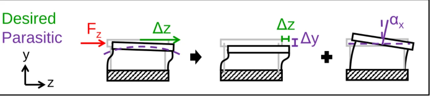
r-compliance element. The graph shows that the ratio is larger than 1 for ϕ>123°, indicating that beyond that sweep angle the flexure can no longer be considered a θ-axis constraint. ... 36 Figure 1.5: A) A Straight-beam compound four-bar system nests two four-bars to remove the y-axis parasitic displacement of the input stage, Δy, while increasing the range of the system, Δz. The nesting also reduces the parasitic rotation of the each of the stages, αx. B) In a curved compound four-bar the input and floating stages are located on different planes, as a result the parasitic displacements of the input stage, Δr and Δθ, are not directly cancelled by the nesting. The parasitic rotations of the two stages, αr and αθ, are also affected by the nesting. The range of the system is increased [7]. ... 37 Figure 1.6: A) Resulting VonMisses stress on a straight-beam flexure compared to the stress of a

curved-beam flexure of the same dimensions under the same loading. The figure shows that the curved beam experiences a stress concentration at the inner radius. This stress concentration has to be captured by the stress model to ensure the designer calculates the maximum stress on the beam [7]. ... 38

Figure 1.7: Simplified design process flowchart followed by the research components necessary to enable the design process for cylindrical flexure systems. ... 39 Figure 1.8: Comparison between the straight-beam version of a system (A) and its cylindrical

flexure counterpart (B). Cylindrical flexures can lead to a more compact design. The wrapping of the beams leads to footprint and volume reductions. ... 41 Figure 1.9: Assembly of concentric cylinders allows for a compact system design [10]. ... 41 Figure 1.10: Cylindrical flexures can be fabricated using a variety of methods including: A)

Lathe with actuated tool (Turning center), B) abrasive water-jet with a rotary axis [11], and C) 3Dprinter. ... 42 Figure 1.11: Common flexure synthesis approaches include: topology synthesis, pseudo-rigid-body modeling, and exact constraint design. The building block approach and FACT are based on the exact constraint design methodology. ... 43 Figure 1.12: Stiffness Ellipses are a visual representation of stiffness ratios. The relative lengths

of the ellipse axis are representative of the magnitude of the stiffness ratio. ... 45 Figure 1.13: Planar and CF element and system examples. ... 46 Figure 1.14: The arc displacement of a straight four-bar is the result of the sum of two parasitic

displacements (purple), Δy and αx, in addition to the desired displacement (green), Δz. A parasitic displacement is an undesired displacement. ... 48 Figure 1.15: CAD model depicting the actuation of the final CF linear guide design. ... 48 Figure 1.16: CAD model depicting the Δx actuation of the CF x-y-θz stage. ... 49 Figure 2.1: Examples of Smith’s hinges of rotational symmetry: A) Disk coupling and B)

Rotationally symmetric hinge [6]. ... 53 Figure 2.2: Awtar and Slocum’s diaphragm single DOF linear bearing [28]. ... 53 Figure 2.3: Chart shows the current knowledge available on curved-beams and the technology

required to enable the design process for cylindrical flexures. This thesis fills the technology gap which has prevented cylindrical flexures from becoming prevalent. ... 54 Figure 3.1: Flexure element coordinate systems. Figure defines the direction of positive

Figure 3.3: FEA corroboration of compliance matrix, predicted displacements under -0.2N Fz load vs. sweep angle, ϕ. The plot compares the curved beam model to an FEA Beam Element model and an FEA 3D solid model. (L=60mm, tr=6.35mm, tz=1mm, 7075Aluminum). ... 60 Figure 3.4: Curvature adjustment factors, ζ, vs. Sweep Angle, ϕ, for a z-compliance flexure. The

plot shows that as the sweep angle approaches zero the curved-beam behaves like a straight-beam. The curvature adjustment factor can be used to define the value of sweep angle below which a beam can be modeled as a straight beam, ϕs. Below ϕ=34° the value of the two dominant displacements, Δz and αr, are within 5% of the straight-beam value. While for ϕ<14° the additional parasitic rotation, αθ, is less that 1/10th the value of the dominant parasitic motion, αr. ... 63 Figure 3.5: Curvature adjustment factors, ζ, vs. Sweep Angle, ϕ, for an r-compliance flexure. The

plot shows that as the sweep angle approaches zero the curved-beam behaves like a straight-beam. The curvature adjustment factor can be used to define the value of sweep angle below which a beam can be modeled as a straight beam, ϕs. Below ϕ=29° the value of the two dominant displacements, Δr and αz, are within 5% of the straight-beam value. While below ϕ=15° the additional parasitic displacement, Δθ, is less that 1/10th

the value of the dominant parasitic displacement, Δr. ... 64 Figure 3.6: Fixed length flexures with increasing sweep angle, ϕ. ... 65 Figure 3.7: A) Flexure beam cross-sectional area indicating the taper angle, Ψ, or deviation from

the desired rectangular cross-section. B) Location of bend axis of the area moments of inertia, Iz and Ir, of a z-compliance element and an r-compliance element. The taper angle shifts the location of the bend axis of Iz. ... 66 Figure 3.8: Normalized taper angle effect on the area moments of inertia, Iz and Ir, and the

torsional stiffness constant, kt, of a z-compliance CF with ϕ=120°. Effect is normalized using the values for Ψ=0°. ... 67 Figure 3.9: Sweep angle, ϕ, effect on the stiffness ratios for a z-compliance flexure with a radial-thickness, tr, to z-thickness, tz, ratio of 10. The stiffness ratios are equal when ϕ=122.56°. (L=60mm, tr=10mm, tz=1mm, 6061 Aluminum). ... 68 Figure 3.10: Effect of tr/tz ratio on the magnitude of the stiffness ratios for a z-compliance flexure

ϕ=122.56° and their magnitude is less than that the ratio of Kz/Kr for a straight-beam of the same dimensions. (L=60mm, 6061 Aluminum). ... 69 Figure 3.11: Sweep angle, ϕ, effect on the stiffness ratios for an r-compliance flexure with a z-thickness, tz to radial-thickness, tr, ratio of 10. The Kr/Kθ stiffness ratio is equal to 1 when ϕ =122.56°. When the Kr/Kθ is greater than 1 the flexure should be considered θ-compliant because this is its lowest stiffness. (L=60mm, tz=10mm, tr=1mm, 7075 Aluminum). ... 70 Figure 3.12: Effect of tz/tr ratio on the magnitude of the stiffness ratios for an r-compliance

flexure (ϕ =122.56°). Plot shows that regardless of the value of tz/tr the Kr/Kθ stiffness ratio is equal to 1 when ϕ =122.56°. (L=60mm, 7075 Aluminum). ... 71 Figure 3.13: tz/tr effect on the stiffness ratios of an r-compliance flexure (ϕ =122.56°). Plot shows

that tz/tr has a significantly greater effect on the Kr/Kz stiffness ratio of a straight-beam flexure compared to a curved-beam r-compliance element. (L=60mm, 7075 Aluminum). ... 71 Figure 3.14 Taper angle effect on the stiffness ratios for a z-compliance flexure (ϕ=120°). Plot

shows that increasing Ψ increases the value of the stiffness ratios. (L=60mm, tr=10mm, tz=1mm, 7075Aluminum). ... 72 Figure 3.15 Taper angle effect on the stiffness ratios for an r-compliance flexure (ϕ=60°). Plot

shows that increasing Ψ decreases the value of the Kr/Kz stiffness ratio but has no effect on Kr/Kθ. (L=60mm, tz=10mm, tr=1mm, 7075Aluminum). ... 73 Figure 3.16 Definition of parasitic (purple) and desired (green) motions for the three types of

cylindrical flexures: A) z-compliance, B) r-compliance, and C) θ-compliance. ... 74 Figure 3.17 Sweep angle, ϕ, effect on the parasitic ratios of a z-compliance flexure. The two

parasitic ratios, αθ/Δz and αr/Δz, are equal when ϕ =118°. (L=60mm, tr=10mm, tz=1mm, 6061 Aluminum) ... 75 Figure 3.18 Sweep angle, ϕ, effect on the parasitic ratios of an r-compliance flexure. The shaded

region highlights the sweep angles (215.5°>ϕ>132.5°) for which the desired motion, Δr, is less than the parasitic motion, Δθ. (L=60mm, tz=10mm, tr=1mm, 7075Aluminum) ... 76 Figure 3.19 Sweep angle, ϕ, effect on the parasitic ratios of a θ-compliance flexure. Above

Figure 3.21 Linearization of tip rotations for a z-compliance flexure (A), and an r-compliance flexure (B). ... 80 Figure 3.22 Sweep angle, ϕ, effect on the eigenvalue parasitic ratios of z-compliance flexure with

tr/tz=10. (L=60mm, tr=5mm, tz=0.5mm, 7075Aluminum) ... 81 Figure 3.23 Sweep angle, ϕ, effect on the eigenvalue parasitic ratios of an r-compliance flexure

with tz/tr=10. (L=60mm, tz=5mm, tr=0.5mm, 7075Aluminum) ... 82 Figure 3.24 Stiffness ratios sensitivity to sweep angle, ϕ, tolerance for a z-compliance flexure vs.

desired sweep angle. Plot shows the percent error from desired value per degree of sweep angle tolerance. (L=60mm, tr=10mm, tz=1mm, 6061 Aluminum) ... 83 Figure 3.25 Stiffness ratios sensitivity to sweep angle, ϕ, tolerance for an r-compliance flexure

vs. desired sweep angle, ϕ. Plot shows the percent error from predicted value per degree of sweep angle tolerance. (L=60mm, tz=10mm, tr=1mm, 7075 Aluminum) ... 84 Figure 3.26 Parasitic ratios sensitivity to sweep angle, ϕ, tolerance for a z-compliance flexure vs.

desired sweep angle. Plot shows the percent error from predicted value per degree of sweep angle tolerance. (L=60mm, tr=10mm, tz=1mm, 6061 Aluminum) ... 85 Figure 3.27 Parasitic ratios sensitivity to sweep angle, ϕ, tolerance for an r-compliance flexure

vs. desired sweep angle. Plot shows the percent error from predicted value per degree of sweep angle tolerance. (L=60mm, tz=10mm, tr=1mm, 7075 Aluminum) ... 85 Figure 3.28 Stiffness ratios sensitivity to taper angle, Ψ, tolerance for a z-compliance flexure vs.

sweep angle, ϕ. Plot shows that the percent error from predicted value depends on the sweep angle of the flexure. (L=60mm, tr=6.35mm, tz=1mm, 7075 Aluminum) ... 86 Figure 3.29 Stiffness ratios sensitivity to taper angle, Ψ, tolerance for an r-compliance flexure vs.

sweep angle, ϕ. Plot shows that the percent error from predicted value depends on the sweep angle of the flexure. (L=60mm, tz=6.35mm, tr=1mm, 7075 Aluminum) ... 87 Figure 3.30 Parasitic ratios sensitivity to taper angle, Ψ, tolerance for a z-compliance flexure vs.

sweep angle, ϕ. Plot shows that the percent error from predicted value depends on the sweep angle of the flexure. (L=60mm, tr=10mm, tz=1mm, 7075 Aluminum) ... 88 Figure 3.31 ADINA FEA beam models used to determine Kθ. A) Neutral position and B) Off-neutral position Δz=1mm. ... 89

Figure 3.32 Off-neutral position effect on the stiffness of a z-compliance flexure vs. sweep angle, ϕ. Plot shows the ratio of the off-neutral position (Δz=1mm) stiffness to the neutral position (Δz=0) stiffness. (L=60mm, tr=10mm, tz=1mm, 7075 Aluminum) ... 90 Figure 3.33 Gauss elimination is used to eliminate degrees of freedom, creating the compliance

matrices for elements under different boundary conditions. ... 91 Figure 3.34 Boundary conditions effect on stiffness ratios vs. sweep angle, ϕ, for a z-compliance

flexure. Plot shows that the stiffness ratios are always equal when ϕ=122.56°. (L=60mm, tr=10mm, tz=1mm, 7075 Aluminum) ... 92 Figure 3.35 Boundary conditions effect on stiffness ratios vs. sweep angle, ϕ, for an r-compliance flexure. Plot shows that when the parasitic rotation αz is constrained, the sweep angle at which the stiffness ratio Kr/Kθ=1 decreases from ϕ=122.6° to ϕ=90°. (L=60mm, tz=10mm, tr=1mm, 7075 Aluminum) ... 93 Figure 3.36 Boundary conditions effect on the parasitic ratios vs. sweep angle, ϕ, for a z-compliance flexure. Plot shows the effect that constraining one parasitic rotation has on the other parasitic ratio. (L=60mm, tr=10mm, tz=1mm, 7075 Aluminum) ... 94 Figure 3.37 Boundary conditions effect on the parasitic ratios vs. sweep angle, ϕ, for an r-compliance flexure. Plot shows the effect that constraining the one parasitic motion, αz or Δθ, has on the other parasitic ratio. For a αz-constrained element the region for which Δr>Δθ is now limited by 96°>ϕ>150°. (L=60mm, tz=10mm, tr=1mm, 7075 Aluminum) ... 94 Figure 3.38 Load location can be used to remove parasitic rotations. A) A straight-beam loaded

along the z-axis experiences a desired motion, Δz, and a parasitic rotation, αx. B) Loading the beam with a Moment about the x-axis, Mx, at the tip of the flexure, produces a rotation, αx, and a displacement, Δz. C) By applying an Fz load on a stage that measures half the length, L, of the beam, an Mx moment is exerted at the tip cancelling the αx rotation. The resulting motion is a pure Δz displacement. ... 95 Figure 3.39 Location of applied load on a z-compliance element. The loading point is defined by

Figure 3.41 Fz load location required to remove the element’s parasitic rotations, αθ and αr. Plot gives the ratios of γ /ϕ and RL/R vs. Sweep Angle, ϕ, for a z-compliance element. γ is measured from the tip of the flexure. ... 98 Figure 3.42 Fr load location required to remove the element’s parasitic rotation given RL=R. Plot

gives the ratio of γ/ϕ vs. Sweep Angle, ϕ, for an r-compliance element. γ is measured from the tip of the flexure. ... 99 Figure 3.43 Resulting moments on r-compliance and θ-compliance elements as a result of

loading at the tip. Both elements experience a single bending moment, mz, when loaded under Fr and Fθ respectively. The bending moment varies along the length of the beam. The position of the resulting moments is given by Rλ, where λ is measured from the tip of the beam. ... 100 Figure 3.44 Maximum stress location, λmax, vs. sweep angle, ϕ, for an r-compliance element

under a pure Fr load. ... 101 Figure 3.45 Maximum stress location, λmax, vs. sweep angle, ϕ, for a θ-compliance element

under a pure Fθ load. ... 101 Figure 3.46 Normalized VonMises stress vs. sweep angle, ϕ, for an r-compliance element. Stress

is normalized using the 3D-solid FEA stress value for a straight-beam of the same dimensions under the same load. ... 102 Figure 3.47 Normalized VonMises stress vs. sweep angle, ϕ, for a θ-compliance element. Stress

is normalized using the 3D-solid FEA stress value for a straight-beam of the same dimensions under the same load. ... 103 Figure 3.48 Normalized range vs. sweep angle, ϕ, for an r-compliance element under an Fr load.

Range is normalized using the range value for a straight-beam of the same dimensions. ... 104 Figure 3.49 Normalized range vs. sweep Angle, ϕ, for a θ-compliance element under an Fθ load.

Stress is normalized using the range value for a ϕ=5° element. ... 104 Figure 3.50 Range/R vs. sweep angle, ϕ, for an r-compliance element under Fr. Dotted line

shows the range/L for a straight-beam element of the same dimensions. ... 106 Figure 3.51 Range/R vs. sweep angle, ϕ, for a θ-compliance element under Fθ. ... 106 Figure 3.52 Resulting moments on z-compliance element as a result of loading at the tip.

Fz. The resulting moments vary along the length of the beam. The position of the resulting moments is given by Rλ, where λ is measured from the tip of the beam. ... 107 Figure 3.53 Maximum stress location, λmax, vs. sweep angle, ϕ, for a z-compliance element

under a pure Fz load. (L=60mm, tr=6.4mm, tz=0.6mm 7075 Aluminum) ... 108 Figure 3.54 Normalized maximum VonMises stress vs. sweep angle, ϕ, for a z-compliance

element. Stress is normalized using the 3D-solid FEA stress value for a straight-beam of the same dimensions under the same load. Plot compares the FEA stress values to the stress calculated by a stress model that considers the bending axial stress and the torsion shear stress on the beam at the base of the beam (Bending & Torsion) and a stress model that gives the stress at λmax (Bending & Torsion λmax). ... 109 Figure 3.55 ADINA FEA images showing the major stress components on a straight-beam

under a A) bending moment and B) a torsional moment. The axial stress, σθθ-mθ, due to twisting is highlighted because it is the missing component from the original stress model, σvon1-z. ... 110 Figure 3.56 Normalized maximum Von Mises stress vs. sweep angle, ϕ, for a z-compliance

element. Stress is normalized using the 3D-solid FEA stress value for a straight-beam of the same dimensions under the same load. Plot compares the FEA stress values to the stress calculated by the three stress models: (i) the bending axial and the torsion shear stress on the beam at the base of the flexure (Bending & Torsion), (ii) the bending and shear stress at λmax, σvon1-z (Bending & Torsion λmax), and (iii) bending and shear stress at λmax with the presented warping correction, σvon2-z (Warping Correction λmax). ... 112 Figure 3.57 VonMises stress for a ϕ=120° z-compliance element. The FEA values for different

length to radial-thickness, L/tr, and radial to z-axis thickness, tr/tz, are plotted along the presented warping corrected stress model. ... 112 Figure 3.58 Normalized range vs. sweep angle, ϕ, for a z-compliance element. Stress is

normalized using the range value for a straight-beam element of the same dimensions under the same loading. ... 113

four-bar is an example of a parallel system. B) Serial systems are characterized by a shared load path. The compliance of the system (1/Ksys) is equal to the sum of the element compliances. A compound four-bar is created by nesting two four-bars in series. ... 117 Figure 4.2: Four-bar system parameters and motions. Fz indicates load along the z-axis and Δz is

the desired displacement. A) Straight four-bar system: The parasitic motions are given by αx and Δy. a indicates the location of Fz relative to ground, and b is the distance between the two flexures. B) The curved four-bar has four undesired motions, αr, αθ, Δr, Δθ. The location of Fz is specified using RL and γ. ... 119 Figure 4.3: Curved compliant four-bar mechanisms. Image shows the coordinate systems for the

two flexures. ... 120 Figure 4.4: Straight four-bar force and moment diagram. Loads and moments on the flexures and

input stage are shown. Fz is the applied load, while Mx is the moment resulting from constraining the flexure tip. The axial forces, Fy, balance the Mx moments on the input stage. ... 121 Figure 4.5: Curved four-bar force and moment diagram. Loads and moments on one end of the

flexures and input stage are shown. Fz is the applied load, while Mr and Mθ are the moments resulting from constraining each flexure tip. The radial forces, Fr, balance the Mθ and the axial forces, Fθ, balance the Mr moment on the input stage. ... 122 Figure 4.6: Curved four-bar parasitics vs. sweep angle, ϕ. The FEA values were calculated using

a 3D-solid model. The two rotations are normalized using the FEA calculated value for ϕ =30°. The plot shows that the beam-based model is inaccurate for low ϕ. (L=60mm, tr=6mm, tz=0.6mm, Lstage=6mm, 7075 Aluminum). ... 123 Figure 4.7: Stage length effect on the curved four-bar parasitics vs. ϕ. Values were calculated

using an FEA 3D-solid model. The parasitics are normalized using the value for the ϕ =30° four-bar with a 2mm stage. ... 124 Figure 4.8: The curvature of the beam leads to a difference in length between the inner and outer

radiuses. This effect in addition to the length of the stage leads to the rotation of the r-axis of the four-bar away from the r-axis of the elements. The rotation angle is given by ω. ... 125 Figure 4.9: ω adjustment vs. L/tr for three different stage sizes. The plot gives the fitted values

Figure 4.10: Corrected curved four-bar parasitics vs. ϕ. The rotations are normalized using the FEA values for ϕ=30°. The dotted lines show the ω=0° model values for αr and αθ. (L=60mm, tr=6mm, tz=0.6mm Lstage=6mm7075 Aluminum). ... 127 Figure 4.11: Corrected curved four-bar αθ vs. ϕ for different L/tr ratios. αθ is normalized using the

FEA value for ϕ=30°. (Lstage = 6mm) ... 127 Figure 4.12: Corrected curved four-bar αr vs. ϕ for different L/tr ratios. αr is normalized using the

FEA value for ϕ=30°. (Lstage = 6mm) ... 128 Figure 4.13: Corrected curved four-bar αθ vs. ϕ for different stage lengths. αθ is normalized using

the FEA value for ϕ=30° with a 2mm stage. The dotted line shows the ω=0° predicted values. (L/tr =10) ... 128 Figure 4.14: Corrected curved four-bar αr vs. ϕ for different stage lengths. αr is normalized using

the FEA value for ϕ=30° with a 2mm stage. The dotted line shows the ω=0° predicted values. (L/tr =10) ... 129 Figure 4.15: Load location effect on the curved four-bar parasitics. Plot gives the normalized

rotations vs. the ratio of RL to R (γ=0°). Rotations are normalized using the FEA values for RL/R=1/6. ... 130 Figure 4.16: Load location effect on curved four-bar parasitics. Plot gives the normalized

rotations vs. the ratio of γ /ϕ. Rotations are normalized using the FEA values for γ=0°. .... 130 Figure 4.17: Applied-moment error effect on αθ. Plot gives the ratio of αθ-resulting/αθ-desired vs.

the ratio of the M-applied to M-desired. ... 131 Figure 4.18: Applied-moment error effect on αr. Plot gives the ratio of αr-resulting/αr-desired vs.

the ratio of the M-applied to M-desired. The dotted line gives the straight four-bar sensitivity to applied-moment error. ... 132 Figure 4.19: Symmetry may be used to cancel the curved four-bar parasitic rotations. ... 132 Figure 4.20: Flexure spacing, b, effect on curved four-bar parasitic motions. Rotations are

normalized using the FEA values for b=10mm. (ϕ=60°) ... 133 Figure 4.21: Input stage Δy displacement for a straight four-bar under Fz. The four-bar’s input

Figure 4.23: The Δr and Δθ parasitic motions of a curved four-bar can be estimated by modeling the curved flexure as a series of straight beams. ... 135 Figure 4.24: Curved four-bar input stage parasitic displacement ratios vs. sweep angle, ϕ. The

plot also compares the FEA calculated parasitic ratios to the model approximations... 136 Figure 4.25: Loading conditions on a CF four-bar flexural element. Mr and Mθ are the moments

applied by the stage constraint on the flexure tip. Fz is the half the load applied on the four-bar. Fz, Mr, and Mθ, produce a bending moment, mr, and a twisting moment, mθ, on the beam. The resulting moments vary along the length of the beam. The position of the resulting moments is given by Rλ, where λ is measured from the tip of the beam. ... 137 Figure 4.26: Curved four-bar Von Mises stress vs. ϕ. Stress is normalized using the stress of a

straight four-bar of the same dimensions under the same load. Plot shows the FEA calculated values, the stress given by a no-warp model and the values given by the full model which includes the warping correction. ... 137 Figure 4.27: A CF compound four-bar is assembled by nesting two four-bars. The input and

floating four-bars have different coordinate systems. If the coordinates of the input four-bar are chosen as the system coordinates, the compliance matrix of the floating four-bar must be transformed to match the system’s new coordinate system (r'2, θ'2, z'2). ... 139 Figure 4.28: In a compound four-bar each four-bar has a different coordinate system; therefore,

an applied radial force, Fr1, on the input four-bar results in radial and axial forces, fr2 and fθ2, and a moment about z, mz, on the floating four-bar. ... 140 Figure 4.29: Sweep angle, ϕ, effect on the CF compound four-bar’s Kz/Kr stiffness ratio. Plot

shows that the ratio decreases with increasing ϕ. The CF’s ratio is compared to the Kz/Kr of a straight compound four-bar of the same dimensions. The graph demonstrates the importance of accounting for the effect of the αz rotation of the floating stage. ... 141 Figure 4.30: Sweep angle, ϕ, effect on the curved compound four-bar’s Kz/Kθ stiffness ratio. Plot

shows that the ratio increases with increasing ϕ. The CF’s ratio is compared to the Kz/Kθ of a straight compound four-bar of the same dimensions. The graph demonstrates the importance of accounting for the effect of the αz rotation of the floating stage. ... 141 Figure 4.31: Curved compound four-bar parasitic ratios vs. ϕ. Plot compares the parasitic ratios

Figure 4.32: Curved compound four-bar parasitic ratios vs. ϕ. Plot compares the parasitic ratios for a compound four-bar to those of a single four-bar. ... 143 Figure 4.33: A symmetric system design may be used to reduce or remove the parasitic

displacements, Δr and Δθ, of a compound bar. A) In a design with two compound four-bars separated by 180°, the Δr displacements cancel out and the Δθ motions result in an αz -rotation. B) Using two double-compound four-bars leads to the cancellation of all the parasitic displacements. ... 144 Figure 4.34: Steps used to establish a CF system’s compliance matrix. +

For serial systems it may be necessary to account for the compliance due to rotations of the secondary stages. ... 145 Figure 5.1: Linear guide prototypes: A) MIT Lincoln Lab’s FTS linear guide, B)First CF linear

guide, C) Second CF prototype designed using CF guidelines. ... 148 Figure 5.2: Michelson Interferometer illustration. A linear guide is used to translate the moving

mirror. ... 149 Figure 5.3: The first CF linear guide prototype was conceived by wrapping two double

compound four-bars. The floating stages of the compound four-bars were joined to create a single cylinder. The CF image highlights the four compound four-bars. ... 150 Figure 5.4: Mechanism used to hold cylindrical stock in place during the machining process used

to create the CF. The future flexure (1) is slipped onto a piece of cylindrical stock (2) which radially supports the work piece. The support stock is attached to a base (3) which is held by the lathe’s spindle. The flexure stock is constrained axially with a cap (4) which is connected to the base using a bolt. ... 152 Figure 5.5: First prototype measurement setup. A) The CF (4) is attached to a grounding cylinder

(3) which is then attached to the optical table. The flexure is actuated using a depth micrometer (1) which pushes on a stage attached to the two input stages of the CF. The inset shows the tip of the micrometer (2) and the actuation stage. B) A cap with scales was attached to the flexure. The displacements of the CF were measured using optical linear encoders: (5) top, (6) center, (7) side. ... 153

Figure 5.7: Tip angle vs. axial displacement (Δz) for the first CF linear guide prototype. The dotted line indicates the functional requirement of 10μradians. A moving average filter (∆z ± 0.3175mm) was used to remove the cyclic behavior imposed by the rotation of the micrometer head... 154 Figure 5.8: FEA analysis of one of the compound four-bars of the first CF linear guide design

shows that the input stage deforms during actuation. ... 155 Figure 5.9: Range vs. sweep angle, ϕ, for a 6061 Aluminum four-bar with R=32mm, tr=6.35mm,

and tz=0.5mm. The minimum range required for the FTS system is 5mm per four-bar which is achieved for ϕ >91°. An R of 31.75mm corresponds to an outer diameter of 69.85mm (2.75”). ... 157 Figure 5.10: Input stage parasitic rotation ratios vs. sweep angle, ϕ, for a 6061 Aluminum

compound four-bar with R=32mm, tr=6.35mm, and tz=0.5mm. Angles below 91° are shaded because they do not meet the minimum 5mm range constraint. The dotted line indicates the FTS 5e-4 rad/m parasitic ratio requirement. ... 158 Figure 5.11: CAD model of the second CF linear guide design. The concept is composed of two

compound four-bars which are labeled in the picture. The design allows for the floating stages to translate and rotate freely. The two compound four-bars’ input stages are joined using connecting rings at the front and back of the cylinder. ... 159 Figure 5.12: Each pocket of the second prototype was filled with putty before the next one was

cut. The putty helps reduce the vibrations of the flexure elements during cutting. ... 160 Figure 5.13: Second prototype measurement setup. A) The CF (4) is attached to a grounding

cylinder (3) which is then attached to the optical table. The flexure is actuated using a depth micrometer (1) which pushes on a cap attached to the connecting ring of the CF. The inset shows the tip of the micrometer (2) and the actuation cap. B) Another cap with scales was attached to the front of the flexure. The displacements of the CF were measured using optical linear encoders: (5) top, (6) center, (7) side. ... 161 Figure 5.14: Tilt angle, αtilt, vs. axial displacement (Δz) for the second CF linear guide prototype.

The dotted lines indicate the functional requirement of ±10μradians. The flexure was actuated using a micrometer. A moving average filter (∆z ± 0.3175mm) was used to remove the cyclic behavior imposed by the rotation of the micrometer head. ... 162

Figure 5.15: Tip angle, αtip, vs. axial displacement (Δz) for the second CF linear guide prototype. The dotted lines indicate the functional requirement of ±10μradians. The flexure was actuated using a micrometer. A moving average filter (Δz ± 0.3175mm) was used to remove the cyclic behavior imposed by the rotation of the micrometer head. ... 162 Figure 5.16: Weight loading measurement setup. The flexure (2) is attached to the table using a

grounding cylinder (1). The CF is loaded using a mass (5) on a low-friction pulley (4). The displacements are measured using the same three optical linear encoders (3). ... 163 Figure 5.17: Tilt angle, αtilt, vs. axial displacement (Δz) for the second CF linear guide prototype.

The dotted lines indicate the functional requirement of ±10μradians from the average tilt error. The flexure was actuated by hanging masses. ... 164 Figure 5.18: Tip angle, αtip, vs. axial displacement (Δz) for the second CF linear guide prototype.

The dotted lines indicate the functional requirement of ±10μradians from the average tip error. The flexure was actuated by hanging masses. ... 164 Figure 5.19: Machining errors: A) Tool lead-in error resulted in some of the flexure elements

being thinner at their base. B) The back connecting ring is larger than the front because of the machine’s travel limit. ... 166 Figure 5.20: Linear guide constructed using two CF bearings. ... 167 Figure 61: A) Thomas’ current straight-beam y-θz stage [35]. B) Proposed CF r-compliance x-y-θz stage. ... 170 Figure 6.2: DPN alignment mechanism with the straight-beam x-y-θz-stage [35]. The camera is

used to determine the position of the DPN tip, while the voice coil actuators are used to position the tip... 171 Figure 6.3: Preliminary CF x-y-θz stage concepts. The table compares the motions of the three

layouts under Fy and Mz loads. The desired displacements are indicated in green, while the parasitic motions are given in purple. ... 173 Figure 6.4: 4-Flexure spider concept. Axi-symmetric layout of the flexures reduces Kθz. In this

sweep angle of the flexure, ϕ, the radial thickness, tr, and the z-axis thickness, tz. The figure also shows the system and element coordinate systems. ... 175 Figure 6.6: Spider concept stiffness ratios vs. element sweep angle, ϕ. Plot shows that Kx/Kz =

Kθz/Kθx when ϕ =60°. (Rsys=3”, Rstage=0.5”, tz=0.5”, tr=0.03”, 6061-T6 Al). ... 177 Figure 6.7: Spider concept in-plane stiffnesses vs. element sweep angle, ϕ. The stiffnesses are

normalized using the desired stiffness value, Kx-desired=1700N/m, Kθz-desired=2Nm/rad. (Rsys=3”, Rstage=0.5”, tz=0.5”, tr=0.03”, 6061-T6 Al). ... 177 Figure 6.8: Serial spider concept design. System is composed of two spider designs connected in

series. The top stage is actuated while the bottom stage is grounded. Each leg of the system is composed of two r-compliance elements connected in series. ... 178 Figure 6.9: Single plane serial spider design. The attachment angle between the serial flexures is

given by ν. The coordinate system for the input-flexure is given by ri-θi-zi, while rg-θg-zg designate the coordinate system for the ground-flexure. The dotted lines delineate the subsystem for which the analysis and optimization was performed. ... 179 Figure 6.10: Flexure attachment angle, ν, effect on the serial spider concept subsystem in-plane

stiffnesses. The stiffnesses are normalized using the corresponding stiffness value for ν =0°. ν must be less than or equal to 60° for both flexures to fit within Rsys. The plot corresponds to a design with ϕ=60°. ... 181 Figure 6.11: Flexure attachment angle, ν, effect on the serial spider concept subsystem stiffness

ratios. The ratios are normalized using the corresponding ratio value for ν =0°. ν must be less than or equal to 60° for both flexures to fit within Rsys. The plot corresponds to a design with ϕ=60°. ... 181 Figure 6.12: Flexure attachment angle, ν, effect on the serial spider concept subsystem in-plane

range. The ranges are normalized using the corresponding range value for ν =0°. ν must be less than or equal to 60° for both flexures to fit within Rsys. The plot corresponds to a design with ϕ=60°. ... 182 Figure 6.13: A) Subsystem Δz displacement under an Fz load. FEA image shows the θx and θy rotations of the subsystem’s stage. B) Full system Δz displacement under an Fz load. The system’s stage does not experience a θx or θy rotation. ... 183 Figure 6.14: Stage attachment angle definition. The attachment angle between the stage and the

Figure 6.15: Stage attachment angle, η, effect on the serial spider concept subsystem in-plane stiffnesses. The stiffnesses are normalized using the corresponding stiffness value for η =0°. The plot corresponds to a design with ϕ=60° and ν =60°. ... 184 Figure 6.16: Stage attachment angle, η, effect on the serial spider concept subsystem stiffness

ratios. The ratios are normalized using the corresponding ratio value for η =0°. The plot corresponds to a design with ϕ=60° and ν =60°. ... 185 Figure 6.17: CF stage first four frequency modes: A) Original design, B) Design with four radial

arms, and C) Design with four arms with masses. ... 187 Figure 6.18: Final CF x-y-θz DPN stage prototype. System was fabricated using an abrasive

water-jet. ... 188 Figure 6.19: CF x-y-θz DPN stage measurement setup. Six capacitance probes (1-6) are used to

measure the three displacements, Δx, Δy, and Δz, and three rotations, θx, θy, and θz, of the stage. The system is actuated by hanging masses off the stage. ... 189 Figure A.1: FEA corroboration of compliance matrix, predicted displacements under -0.2N Fθ

load vs. sweep angle, ϕ. The plot compares the curved beam model to an FEA Beam Element model and an FEA 3D solid model. (L=60mm, tr=6.35mm, tz=1mm, 7075Aluminum). ... 199 Figure A.2: FEA corroboration of compliance matrix, predicted displacements under -0.2N Fr

load vs. sweep angle, ϕ. The plot compares the curved beam model to an FEA Beam Element model and an FEA 3D solid model. (L=60mm, tr=6.35mm, tz=1mm, 7075Aluminum). ... 200 Figure A.3: FEA corroboration of compliance matrix, predicted displacements under -3.175Nmm Mz vs. sweep angle, ϕ. The plot compares the curved beam model to an FEA Beam Element model and an FEA 3D solid model. (L=60mm, tr=6.35mm, tz=1mm, 7075Aluminum). ... 201 Figure A.4: FEA corroboration of compliance matrix, predicted displacements under 10Nmm Mr vs. sweep angle, ϕ. The plot compares the curved beam model to an FEA Beam Element model and an FEA 3D solid model. (L=60mm, tr=6.35mm, tz=1mm, 7075Aluminum). ... 202 Figure A.5: FEA corroboration of compliance matrix, predicted displacements under 10Nmm Mθ

T

ABLES

Table 3.1: Average model error and standard deviation for each displacement ... 60 Table 3.2: Primary (PCV) and secondary compliance vectors (SCV) for a z-compliance flexure.

Vectors depend on the sweep angle, ϕ. (L=60mm, tr=5mm, tz=0.5mm, 7075 Aluminum) .... 81 Table 3.3: Primary (PCV) and secondary compliance vectors (SCV) for an r-compliance flexure.

Vectors depend on the sweep angle, ϕ. (L=60mm, tz=5mm, tr=0.5mm, 7075 Aluminum) .... 82 Table 3.4: Range of values used for each of the components included in the stress model

parametric study. ... 111 Table 5.1: FTS linear guide functional requirements. ... 149 Table 5.2: First CF linear guide prototype dimensions... 151 Table 5.3: First CF linear guide prototype performance. +Error over 5mm range. ... 156 Table 5.4: Second CF linear guide prototype dimensions. ... 159 Table 5.5: Second CF linear guide prototype performance. +Error over 5mm range. ... 165 Table 5.6: Possible sources of tip/tilt error. +Error over 5mm range. ... 166 Table 6.1: DPN x-y-θz-stage attributes. ... 171 Table 6.2: Advantages and disadvantages of the preliminary CF x-y-θz stage concepts. ... 173 Table 6.3: Final CF x-y-θz-stage element and system parameters. ... 185 Table 6.4: Performance comparison for the straight-beam and CF x-y-θz-stages. ... 186 Table 6.5: CF DPN x-y-θz stage performance. ... 189

C

HAPTER

1

I

NTRODUCTION

1.1 Synopsis

Compliant mechanisms, or flexures, guide motion through member compliance. They are powerful machine elements, because unlike rigid mechanisms they have no sliding joints therefore they do not experience stick and slip due to friction. Compliant mechanisms are prevalent in engineering because design guidelines have been developed that inform the engineer as to how to design the flexure to obtain the correct kinematics and ensure that the system achieves the desired range. No such rules exist for guiding the design of the curved-beam elements utilized in cylindrical flexures (CFs). The focus of this research is to develop the design rules and models necessary to enable to synthesis and optimization of CFs. These new flexures systems may be utilized to create more compact, lower cost solutions, which are particularly necessary for applications constrained to a cylindrical geometry.

This thesis presents the four fundamental contributions required to enable the design process for CFs: (i) analysis of element mechanics models to reveal key parameters, (ii) development of an accurate stress model to predict element and system range, (iii) understanding of how the key parameters affect the flexure performance and (iv) guidelines as to how to assemble and optimize CF systems. The impact of this work is demonstrated through two case studies, shown in Figure 1.1. The need for design rules and models is most evident when one attempts to design a CF system using the available straight-beam models and finds that they are inadequate. Without design rules the engineer is forced to rely on FEA and blind iteration. The contributions of this thesis enabled the rapid design and optimization of these CF systems, reducing the design process timeline from months to weeks.

Figure 1.1: Two cylindrical flexure system examples: (A) linear guide and (B) x-y-θz stage.

1.2 Cylindrical Flexures

The resolution of sliding joints is limited to 100s of nanometers because of the stick-slip phenomenon, making friction bearings inadequate for precision motion applications. Flexures on the other hand can attain angstrom level resolution because they achieve motion through member compliance; therefore they do not suffer from friction. Compliant mechanisms must operate within their elastic deformation range to ensure the repeatability of the system. As a result, flexure elements must be operated below their yield stress which limits a flexure’s range and load capacity [5], [6]. Another advantage of compliant mechanisms is that they can preclude assembly and fabrication costs because they can be created from a single piece of stock.

Current flexure systems are mostly planar; this limits their uses and their impact. Straight-beam flexures are common because design rules have been established which enable their effective design. However, no such rules exist for CFs, and therefore the design process is impeded. Cylindrical compliant mechanisms could fill the gaps that current planar flexures fail to meet. Some of the CF benefits include: (i) the availability of precision round stock, means reduced fabrication variations and (ii) reduced cost, (iii) compatibility with cylindrical

1.2.1 Definition

Herein I define CFs as systems with flexure elements that have only one finite radius of curvature, in other words, systems composed of flexure beams that are curved in a single plane. Figure 1.1 shows two examples of CF systems, a linear guide and an x-y-θz stage. Chapter 5 presents how the design rules developed in this work were used to improve the performance of the CF linear guide. The conception of the curved-beam x-y-θz stage is covered in Chapter 6. Past works have given different names to flexures that fall under the CF description. The most applicable definition is Smith’s “hinges of rotational symmetry”, which he characterizes as flexures constructed from solids of revolution [6]. In this work Smith’s definition is expanded to allow CFs to be fractions of a solid of revolution. The thesis is scoped by constraining CFs to systems formed by elements with a single finite radius. Finally, the system must have well-defined distortions for it to be classified as a CF.

Two types of flexural blade elements may be constructed under the given CF definition. The element types, shown in Figure 1.2, are classified by their direction of least stiffness, (A) z-compliance and (B) r-z-compliance. The coordinate system of the element is defined at its tip using cylindrical coordinates. The length of the flexure is given by Rϕ, where R is the radius of curvature and ϕ defines the sweep angle of the element. The flexure’s radial thickness is given by tr, and its z-axis thickness by tz. The two element types are differentiated by the relative magnitude of their two area moments of inertia, Ir and Iz. A z-compliance element is more compliant in the z-direction because Ir<<Iz; while an r-compliance CF is characterized by Iz<<Ir.

Figure 1.2: Cylindrical flexure elements are defined by their direction of greatest compliance. Their coordinate system is given in cylindrical coordinates at the tip of the

flexure. The flexure blade element is described by its radius, R, sweep angle, ϕ, radial thickness, tr, and z-axis thickness, tz. Z-compliance elements are differentiated from

r-compliance elements by the relative magnitude of their area moments of inertia.

1.3 Cylindrical Flexure Challenges

1.3.1 Element Level Challenges

This section presents a couple of examples of how CF elements behave differently than straight-beam flexures. These differences make current design guidelines inadequate for the effective creation of CF concepts. An example of how the behavior of a curved-beam diverges from that of a straight-beam is given in Figure 1.3 [7]. The image shows the motions of a z-compliance cantilever curved beam loaded at its free-end. In this case, the desired motion is a displacement along the cylinder’s axis, Δz. All other displacements are defined as parasitic motions. The curvature of the beam leads to two parasitic rotations, αr and αθ, compared to one for a straight-beam flexure, αx. In addition, instead of the beam experiencing a single bending

z-compliance

z

r

θ

ϕ

R

t

_r

I

_z

>>I

_r

r-compliance

r

z

θ

t

_z

I

_r

>>I

_z

Figure 1.3: Element level challenges. Straight-beam flexure elements (A) under a z-axis load, Fz, suffer from one parasitic rotation, αx, in addition to the desired displacement,

Δz. The straight flexure experiences a single bending moment, mx. Cylindrical flexure z-compliance elements (B) under a z-axis load, Fz, suffer from two parasitic rotations, αr

and αθ, in addition to the desired displacement, Δz. The curved beam is subjected to a twisting moment, mθ, and a bending moment, mr [7].

Planar flexure blades are characterized by having a single translational degree-of-freedom (DOF). Analysis of the kinematics of an r-compliance CF element provides another example of how the behavior of the curved-blade is different from its straight-beam counterpart. Figure 1.4 plots the ratio of Kr to Kθ stiffnesses vs. ϕ for an r-compliance element. The plot shows that for ϕ>123° the stiffness of the blade along the θ-axis is less than its r-stiffness. In fact, at ϕ=122.56° Kr=Kθ, which means that the CF blade has two translational DOF. In order to capture the kinematics of the r-compliance element using straight-beam models, the curved-beam would have to be approximated as a series of two straight-blades attached at 90°. The analytical models in this thesis present a more accurate way to model the behavior of the r-compliance curved blade.

m_x F_z α_x ∆z x y z F_z α_r α_θ m_r m_θ ∆z z θ r A B

Figure 1.4: Sweep angle effect, ϕ, on the ratio of r-axis stiffness, Kr, to θ-axis stiffness, Kθ, for an r-compliance element. The graph shows that the ratio is larger than 1 for ϕ>123°, indicating that beyond that sweep angle the flexure can no longer be considered a θ-axis

constraint.

1.3.2 System Level Challenges

The curvature of the flexure beams also leads to challenges in the assembly of CF systems. The need for system creation rules is demonstrated by analyzing the behavior of a curved compound four-bar system [7]. A planar compound four-bar, shown in Figure 1.5a, is an example of a parallel and a serial flexure system. The mechanism utilizes two nested four-bar flexure systems to increase the range of the system and mitigate the parasitic displacement, Δy1, of the input stage as shown in Figure 1.5a. The Δy motion of the floating stage cancels the Δy of the input stage. The nesting of the four-bars also reduces the parasitic rotation, αx, of the input stage. In the curved compound four-bar system, shown in Figure 1.5b, the floating and input stages are located on different planes due to the curvature of the beams. As a result of the location of the stages the parasitic displacements, Δr1 and Δθ1, of the input stage are not directly cancelled by the Δr and Δθ of the floating stage.

0 60 120 180 240 300 360 0 1 2 3 4 5 Kr/K R at io

Figure 1.5: A) A Straight-beam compound four-bar system nests two four-bars to remove the y-axis parasitic displacement of the input stage, Δy, while increasing the range of the system, Δz. The nesting also reduces the parasitic rotation of the each of the stages, αx. B) In

a curved compound four-bar the input and floating stages are located on different planes, as a result the parasitic displacements of the input stage, Δr and Δθ, are not directly cancelled by the nesting. The parasitic rotations of the two stages, αr and αθ, are also

affected by the nesting. The range of the system is increased [7].

The mitigation of the parasitic rotations of the input stage, αr1 and αθ1, is also not straight forward. For example, in the case where ϕ=90° the αr of the floating stage corresponds to a αθ of the input stage and vice versa. This leads to having to manage eight parasitic motions (four for each stage) on two different planes. The matter of mitigating these motions is no longer clear; the rules that have been established for straight-beam systems are inadequate for CFs. This work presents models and guidelines that enable the efficient design of curved parallel and serial CF systems like the curved compound four-bar.

1.3.3 Stress Concentration

In order to determine the range of a system both the displacement under a given load and the resulting stress must be considered. The curvature of a z-compliance element leads to a

2Δz A B Floating Stage Input Stage Δy₁ Δz Δy₂ Δz α_x1 α'_x1 α'_x2 α_x2 Δθ₁ Δz Δr₁ y z r₁ z₁ θ₁ α_θ1 αr1 Δr₂ Δz Δθ2 α_r2 α_θ2 Δθ'₁ Δr'₁ α'_r1 α'_θ1 Δr'₂ Δθ'₂ α'_r2 α'_θ2 2Δz r₂ θ₂ z₂

Desired

Parasitic

twisting moment on the fixed end of the cantilever beam. This moment will affect the resulting stress calculation. Using energy conservation principles it can be identified that an added twisting moment requires that there be a decrease in the original resulting bending moment. Both of these effects will change the magnitude and distribution of the stress along the beam. Figure 1.6 shows that a stress concentration is observed at the base on the inner radius of the z-compliance curved element [7]. The stress model for the straight-beam flexure does not predict the stress concentration and therefore underestimates the stress level in the deflected beam. A stress model for the curved-beam flexure needs to be developed to ensure the accurate assessment of the range of the CF.

Figure 1.6: A) Resulting VonMisses stress on a straight-beam flexure compared to the stress of a curved-beam flexure of the same dimensions under the same loading. The figure

shows that the curved beam experiences a stress concentration at the inner radius. This stress concentration has to be captured by the stress model to ensure the designer

calculates the maximum stress on the beam [7].

1.4 Design Process

The main steps of the engineering design process are summarized in Figure 1.7. First the designer must establish the functional requirements for the system. Once the requirements have been formulated the next step is to generate possible concepts that would meet those needs. This step is often called preliminary design because the designer is generating abstract embodiments

Von Misses Stress (N/m2₎ 7.3e7 1.2e4 4.9e7 2.5e7 10mm

considering different solutions and continuing with the least limiting design. During the detailed design step the selected concept is optimized given a set of criteria. Finally, once the design is complete the system can be fabricated.

Figure 1.7: Simplified design process flowchart followed by the research components necessary to enable the design process for cylindrical flexure systems.

Design rules play a significant role in the compliant mechanism design process. In planar flexure design the generation of concepts is facilitated by using guidelines that establish the degrees-of-freedom (DOF) and constraints of a flexure element. This knowledge allows the designer to quickly layout different compliant elements to achieve the desired system motions. The straight-beam design rules are used in the concept analysis and selection phase to establish order of magnitude estimates of parasitic motions and range to footprint ratios. These assessments are used to efficiently compare the performance of a concept relative to the other ideas. Once the most promising concept has been selected the straight-beam models provide the engineer with the knowledge required for the effective optimization of the concept. Optimization can be a tedious process if the designer does not understand the effect of the different flexure parameters on the system performance metrics.

Section 1.2 established that the current straight-beam flexure design rules and models are insufficient for the successful design of CFs. The lack of design guidelines restricts the CF design process. Figure 1.7 summarizes the research that must be conducted to enable the design process. Foremost, the kinematic behavior of a curved-beam element has to be understood and modeled. The analytical models may then be used to characterize the effect of different parameters on the behavior of the beam. The parameters that differentiate the behavior of the curved-beam from that of a straight-beam must be identified as key parameters. The concept

Concept Generation Building

blocks

Optimization

Element Mechanics and Key Parameters Stiffness Representation

System Creation Guidelines Fab. Guidelines Identify DOF and Constraints Analysis and Selection Fabrication System Creation Enabling Research