Development of an automated efficiency and loss measurement system for high-efficiency power converters

Development of an Automated Efficiency and Loss

Measurement System for High-Efficiency Power Converters

by

Grace M. Cheung

S.B., Massachusetts Institute of Technology (2009)

Submitted to the Department of Electrical Engineering

and Computer Science

in Partial Fulfillment of the Requirements for the Degree of

ARCHIVES

MASSACHUSETTS INSTITUTE

Master of Engineering in Electrical Engineering

and Computer Science

AUG 2 4 2010

at the

_LIBRARIES

MASSACHUSETTS INSTITUTE OF TECHNOLOGY

June 2010

@ Massachusetts Institute of Technology 2010. All rights reserved.

A uthor...

i)De ment of Electrical Engineering

and Computer Science

June 1, 2010

Certified

by...----.--.--David J. Perreault

Associate Professor

Thesis Supervisor

Christopher J. Terman

Chairman, Department Committee on Graduate Theses

Development of an Automated Efficiency and Loss

Measurement System for High-Efficiency Power Converters

by

Grace M. Cheung

Submitted to the Department of Electrical Engineering

and Computer Science on May 21, 2010, in Partial Fulfillment of the Requirements for the Degree of

Master of Engineering in Electrical Engineering and Computer Science

Abstract

When building a high performance power converter system, characterization becomes a significant task in and of itself. This thesis addresses the development of an automated efficiency and loss measurement system for high-efficiency power converters. The design, construction, calibration, and evaluation of such a measurement setup is described, including development of software to control the system. Application of the setup to a solar high- efficiency grid-tie inverter system is also addressed.

Thesis Supervisor: David J. Perreault Title: Associate Professor

Acknowledgements

I thank my thesis advisor, Dr. David J. Perreault, for the past four years of guidance and support.

Thanks to Paul E. Gray, for being an excellent academic advisor and mentor, and for always believing in me.

Thank you to Brandon Pierquet and Aleksey Trubitsyn, with whom I worked with on this project.

Thanks to Tony Eng and the MIT EECS department for funding me through a 6.UAT teaching assistantship.

I am grateful for all the help provided by my colleagues in Dave's group and in LEES, most

notably Uzoma Orji and Shahriar Khushrashahi, as well as Yehui Han, Wei Li, and JianKang Wang.

I would like to give a special thanks to Daisy, the "brother" of my soul. I can still remember

when we first met, you with the dyed green hair, and me, suffering from pneumonia. You have been my accomplice through thick and thin, and to know you has been my biggest pride. This work is dedicated to my friends who have supported me throughout my years at MIT: Jennifer Shar, Kenny Donahue, Sherry Gao, Juan Rivas, Anthony Sagneri, Jackie Hu, and George Hwang. We have shared very special memories that I will always treasure. You were there when I was up, and more importantly, you were there when I was down. Thank you for being who you are, and for being my friends.

I owe my deepest gratitude to my sister and my parents, without whose support I would not be

Contents

Chapter 1. Introduction ... 15

1.1. Solar High-Efficiency Grid-Tie Inverter System... 16

1.1.1. CEC Efficiency ... 17

1.1.2. Choosing Operating Points ... ... 18

1.2. Automation of Hardware... 18

1.3. Organization of the Thesis ... 20

Chapter 2. Efficiency and Accuracy Calculation ... 23

2.1. Sources of Error in Agilent 34401A... 23

2.1.1. Measurement Noise and Offset... 23

2.1.2. Multimeter Accuracy ... 24 2.2. Error Analysis... 26 2.2.1. Derivation Method ... ... 26 2.2.2. Root-Sum-Squares Method... 27 2.2.3. Interval Analysis ... . 28 2.3. Efficiency A nalysis ... .- -... 29

2.3.1. Determ ining Operating Points ... 30

2.4. Example of Error Propagation in Measurement System... 31

2.4.1. Operating Point with Efficiency Calculation... 32

2.4.2. Current Shunt on Output Current Measurement Analysis... 33

3.1. Need for A utom ation... ₃₅

3.2. Autom ation Algorithm ... ₃₈

3.3. q p p ... ₄₀

Chapter 4. System Test and Validation... ₄₃

4.1. Control M easurem ents ... 44

4.2. Autom ated M easurem ents... 46

4.2.1. _{Test 1: Sweeping All Possible Voltages ... 46}

4.2.2. Test 2: Sweeping All Possible Input Currents ... 55

4.3. Solar M icro-Inverter Test Data Analysis ... 59

Chapter 5. Sum m ary and Conclusions... 69

5.1. Thesis Conclusions... ₆₉

5.2. Thesis Sum m ary ... ₆₉

5.3. Future W ork ... ₇₁

Appendix A M aster Loop Code ... 73

Appendix B Associated Functions Code... 83

B . Opening the Port... 83

B2. Interval M ultiply Code ... 83

B3. Interval Divide Code ... 84

B4. Comparison of Current Measurement using Multimeter with and without Current Shunt... ₈₄

B5. Error Bars on Input and Output Voltages... 85

B6. Error Bars on Output Current ... 86

B7. Error Bars on Input Current... 87 8

Appendix C Generating Operating Points for Solar Micro-Inverter...89

C1. Code to Determine Operating Points... 89

C2. First Few Samples from List of Generated Operating Points (PPT Matrix)... 90

Appendix D Data Points from Automated Tests ... 91

D 1. Code for A nalyzing D ata... 91

D2. Test 1: Input Voltage and Error Bars, Input Current and Error Bars ... 92

D3. Test 1: Output Voltage and Error Bars, Output Current and Error Bars... 94

D4. Test 1: Input Power and Error Bars, Output Power and Error Bars... 96

D5. Test 2: Input Voltage and Error Bars, Input Current and Error Bars ... 98

D6. Test 2: Input Power and Error Bars... 98

List of Figures

Figure 1-1: Circuit Topology of Solar Micro-Inverter ... 17

Figure 1-2: Overall System Block Diagram ... 20

Figure 3-1: Hardware Automation Algorithm... 39

Figure 3-2: Overall System Diagram... 42

Figure 4-1: Resistor Test Board Topology ... 43

Figure 4-2: Test 1 Input Voltage Measurement... 48

Figure 4-3: Test 1 Input Voltage Measurement Zoomed in ... 49

Figure 4-4: Test 1 Input Current Measurement ... 50

Figure 4-5: Test 1 Output Voltage Measurement ... 51

Figure 4-6: Test 1 Output Current Measurement... 52

Figure 4-7: Test 1 Input Power Calculation... 53

Figure 4-8: Test 1 Output Power Calculation... 54

Figure 4-9: Test 2 Input Voltage Measurements ... 56

Figure 4-10: Test 2 Input Current Measurements... 57

Figure 4-11: Test 2 Input Power Calculations ... 58

Figure 4-12: Test Data Input Voltage Measurement ... 61

Figure 4-13: Test Data Input Current Measurement... 62

Figure 4-14: Test Data Output Voltage Measurement... 63

Figure 4-15: Test Data Output Current Measurement ... 64

Figure 4-16: Test Data Input and Output Power Calculations... 65

List of Tables

Table 1.1: Specifications for Solar Micro-Inverter... 17

Table 1.2: List of Equipment Used... 19

Table 2.1: Agilent 34401A Accuracy Specifications ± (% of reading + % of range)... 25

Table 2.2: Agilent 34330A Accuracy Specifications ... 25

Table 2.3: CEC Coefficient W eights ... 30

Table 2.4: Sample Data for Solar Micro-Inverter... 32

Table 2.5: Sample Data with Uncertainty and Ranges for Measured Values... 32

Table 2.6: Input, Output Power and Efficiency Range for Sample Data... 33

Table 2.7: Comparison of Accuracy with and without Current Shunt ... 34

Table 3.1: Six Different Average Power Levels... 36

Table 3.2: Three Different Input Voltage Levels... 36

Table 3.3: Fifteen Different Output Voltages ... 37

Table 3.4: Equipm ent List... 40

Table 4.1: Resistor Values and Limits for Test Board... 44

Table 4.2: Control Operating Points ... 45

Table 4.3: Control Measurements and Power Calculation ... 45

Table 4.4: Operating Voltages for Automated Test 1... 46

Table 4.5: Maximum Uncertainty for Automated Measurements Test 1 ... 54

Table 4.6: Operating Input Currents and Associated Input Voltage, for Rin = 1.6Q ... 55

Table 4.7: Maximum Uncertainty for Automated Measurements Test 2 ... 58

Table 4.8: Sample Test Data for Solar Micro-Inverter ... 60

Table 4.9: Calculated Efficiency for each Average Power Level... 67

Chapter 1.

Introduction

Measurement is the process of assigning values to describe observed properties of phenomena. Although seemingly trivial, measurements become increasingly difficult to make when a high level of accuracy is demanded. A measurement is only as good as its measurement system, which depends heavily on the precision of the equipment, technique of acquiring data, and analysis of results. All of these contribute to error, which makes uncertain the true value of the variable measured [1].

Thorough uncertainty analysis allows for the reporting of measured values with confidence. It is comprised of two main components: systematic and random. Systematic uncertainty arises in calibration issues and bias. It encompasses initial design errors, such as instrument selection, data acquisition methodology, and other considerations that need to be undertaken prior to actually performing the measurement. Random uncertainty refers to errors that exist due to repetition in procedure and condition [2].

Measuring the behavior and efficiency of power conversion systems can be challenging, especially when the efficiency of the circuit is high. Small differences in large numbers have a significant impact on calculating efficiency and loss when losses are measured as the difference between input and output power. Small errors in one measurement can propagate to a staggeringly inaccurate calculation of important power converter characteristics, such as efficiency and loss. In order to calculate the efficiency of a converter, one must measure the input and output voltages, as well as the input and output currents. A 1% error in any one of these four measurements leads to an approximately 1% error in calculated efficiency. For a high efficiency converter (e.g. 98% nominal), this can represent as much as a factor of two error in calculated loss. Thus, being able to take measurements accurately, although difficult, becomes very desirable.

Automation is important for improving accuracy and increasing effectiveness. When recording voltage and current data by hand, there exists a time lag between reading the voltage and reading the current. For power systems in which the operating point moves slightly over time, recording data by hand this way results in incorrect associations of voltage and current. This propagates to errors in calculating the efficiency and loss. Automating the system allows for simultaneous readings of voltages and currents, which eliminates this time lag and fixes this problem.

There are also major advantages to automating measurements of systems that have to be evaluated across a wide range of operating conditions. For example, in measuring the efficiency of micro-inverters for photovoltaic applications, at least forty different operating points must be measured to provide a data set for one power level for efficiency calculation. For each operating point, four measurements are taken of the input voltage and current, and the output voltage and current. This comes out to at least one hundred and sixty measurements that must be taken at each power level. Doing this by hand becomes tedious and introduces error, so automation becomes increasingly attractive.

The goal of this thesis is to develop an automated system for measuring the efficiency and loss of high-efficiency power converters.

1.1. Solar High-Efficiency Grid-Tie Inverter System

The measurement system proposed here will be implemented for measuring high-efficiency grid-tie inverters for photovoltaic (PV) applications, but is meant to be easily generalized to similar converter systems, including power converters with more than two ports. The circuit topology for the first inverter to be tested is shown in Figure 1.1 [3],[4],[5].

PV+ .. II

AO B' HF

Transformer Full Bridge

~~---n~vsrtr~ ~ ~~C cidir

Figure 1-1: Circuit Topology of Solar Micro-Inverter

This solar micro-inverter, presented in [4], [5], and [6], has the following specifications:

Input Voltage 25V -40V dc

Output Voltage 240V ac RMS Maximum Output Power 175 W

Efficiency > 97% C.E.C

Table 1.1: Specifications for Solar Micro-Inverter.

1.1.1.

CEC Efficiency

The efficiency cited follows the metrics outlined by the California Energy Commission

(CEC) for rating efficiency. The CEC considers the efficiency of a PV inverter as a weighted

average of its efficiency at six different power and input voltage levels, expressed as percentages of the maximum average power. The proposed system will measure the voltage and current at each port to calculate the average power. Following the CEC's metric of efficiency, the converter will be run over a wide range of operating points, across input voltage, line cycle position, and power levels.

The voltage and current will be measured at multiple ports for the ranges of interest, and will go into calculating the output power and CEC efficiency. A more detailed look at the CEC efficiency calculation is presented in Chapter 1.

The inverter application does not require measuring efficiency by looking at ac. Instead, discrete points along the line cycle are picked and evaluated. These then are used to calculate the overall efficiency of the inverter by integrating over the line cycle.

1.1.2.

Choosing Operating Points

Let the term "operating point" be defined as a unique point on the ac line cycle for a given input voltage and power component to the converter. This means an operating point defines the input voltage, output voltage, and instantaneous power over the line cycle.

Each of the three input voltage levels has to sweep through fifteen output voltage levels. This process is repeated for each of the six average power levels. Overall, this produces an estimated one thousand individual measurements, which drives the need for automation.

1.2. Automation of Hardware

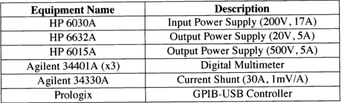
The control system sets the operating point, records data, and archives that data. The micro-inverter setup utilizes the following equipment:

Equipment Name Description

HP 6030A Input Power Supply (200V, 17A) HP 6632A Output Power Supply (20V, 5A) HP 6015A Output Power Supply (500V, 5A) Agilent 34401A (x3) Digital Multimeter

Agilent 34330A Current Shunt (30A, 1mV/A)

Prologix GPIB-USB Controller

Table 1.2: List of Equipment Used

The dc input voltage, and the voltages at one or more output ports must be varied. In order to do this, operating commands to the power converter itself are developed, as well as methods for driving and loading the converter in an automated fashion.

On the output side of the solar micro-inverter, the HP 6015A is able to reach 240V, but lacks GPIB control. However, it does have analog programming capabilities. Thus, the HP

6632A, which has GPIB ability, is connected to the HP 6015A and controls the output voltage of

the HP6015A from commands sent by the computer.

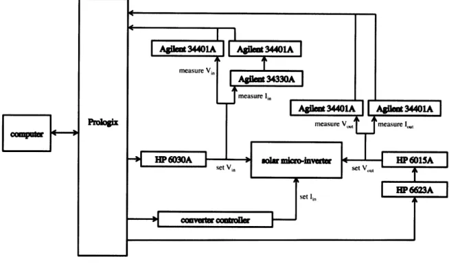
The GPIB commands to all the power supplies set their voltages and currents, which are verified by the multimeters that feed back to the computer. Input current levels reach as high as 14A, which exceeds the current limit ratings on the Agilent 34401A. Thus, the Agilent 34330A current shunt is included to measure the input current. The final setup is represented in the following block diagram:

Figure 1-2: Overall System Block Diagram

1.3. Organization of the Thesis

Chapter 2 explores how efficiency is measured and loss calculated. A discussion follows on sources of error outside of the power converter itself, such as error introduced by the hardware, and how these errors propagate.

Chapter 3 describes the automation and synchronization of all the hardware. This control scheme, although specifically designed for the solar micro-inverter, can be easily modified to accommodate any power converter.

Chapter 4 discusses the testing performed on the system to evaluate the measurement setup and validate its accuracy. A resistor test board is used to compare manual measurements to automated measurements. Sample test data acquired from the solar micro-inverter is analyzed

using the CEC efficiency half of the automation script. The hand-calculated CEC efficiency is compared to the result outputted by the automation script.

Chapter 5 summarizes the thesis and suggests directions for continued work based on the limitations of this system.

The appendices document all the MATLAB script and data generated in the validation tests. Appendix A contains the script that controls the whole measurement system. Appendix B includes the necessary functions called on by the master loop measurement system. Appendix C lists all the possible operating points for the solar micro-inverter. Appendix D shows the data points generated by the automated tests described in Chapter 4. Appendix E comprises of the

CEC calculation part of the automation code, which was run on sample test data from the solar

Chapter 2.

Efficiency and Accuracy Calculation

This chapter discusses the error introduced by the hardware, how this error propagates, and what that means for calculating efficiency. Three methods for calculating error propagation are investigated and analyzed.

2.1. Sources of Error in Agilent 34401A

There are two major sources of error in this measurement system. The first is the offset error, and the second is noise in the measurement. Both of these come from the multimeters, which have accuracy specifications that make it easier to quantify the error.

2.1.1.

Measurement Noise and Offset

Offset error is inherent and is hard to remove unless the equipment is taken in for calibration. Even then, after some time has passed, offset creeps back in. Although offset poses a problem, it does stay consistent, which means measurements with offset will remain relatively accurate, if not absolutely accurate. Consider a voltage measurement that initially reads

10.0356V and then a later voltage measurement reads 22.4598V. It can be said with certainty

that the voltage has increased, even if the absolute values of those readings cannot be deduced. Measurement noise is modeled as Gaussian, and thus can be eliminated by the Root-Sum Squares Method, introduced in Section 2.2.2. This is essentially eliminated by the multimeter itself, since the Agilent 34401A has built in functionality to take long term measurements and internally average them to significantly reduce measurement noise.

Another source or error, although not as prominent, is error incurred with changes in temperature. One way to overcome this is by trying to keep the temperature constant, which means operating the hardware at its steady state, after it has warmed up to some asymptotic temperature. This will cause the drift rate to be small, and thus cut out error associated with temperature change. However, this does not make the reading more accurate, but instead, more consistent.

2.1.2.

Multimeter Accuracy

The three power supplies used (HP 6030A, HP 6015A, and HP 6632A) may have error in the sense that the value each indicates it is outputting is not the real voltage value sourced. Since multimeters are used to measure the real voltages and currents inputted and outputted from the power converter, and it is these measured values which are used to calculate power and efficiency, and thus that power supply error is not a problem, and does not factor in to the overall analysis of the measurement system.

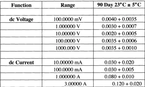
However, the multimeters themselves have error in that they have accuracy limitations, and this does indeed play a big role. The Agilent 34401A has a different error associated with its measurement depending on the voltage level, frequency, and type of measurement. The accuracy specifications are summarized in the following table [6]:

Function Range 90 Day 23*C ± 5*C dc Voltage 100.0000 mV 0.0040 + 0.0035 1.000000 V 0.0030 + 0.0007 10.00000 V 0.0020 + 0.0005 100.0000 V 0.0035 + 0.0006 1000.000 V 0.0035 + 0.0010 dc Current 10.00000 mA 0.030 + 0.020 100.0000 mA 0.030 + 0.005 1.000000 A 0.080 + 0.010 3.00000 A 0.120 + 0.020

Table 2.1: Agilent 34401A Accuracy Specifications t (% of reading + % of range)

The uncertainty is comprised of two parts, the first being the percentage of the reading, and the second the percentage of the range. For example, consider the case where the Agilent 34401A reads a dc voltage level of "33.2345mV." The error associated with this measurement is: ±[(0.000040*0.0332345)+(0.000035*0.1)]= +4.82938e-6 V, which is 0.01453% of the nominal 33.2345mV value.

The current shunt reads out a voltage proportional to the amount of current it measures,

by a 1mV/A ratio. The accuracy specifications for the Agilent 34330A is summarized below [7]:

Frequency Range Uncertainty

dc - 1kHz 0.3%

1kHz-5kHz 5%

Table 2.2: Agilent 34330A Accuracy Specifications

The 1kHz-5kHz range gives a very substantial 5% error, but since all measurements taken are at dc, the error introduced from the shunt is always only 0.3%. However, it is important

to realize that this is extra error added on to the error from the multimeter, not the overall error for the current measurement. Take, for example, a dc current measurement using the Agilent 34401A and the Agilent 34330A. If the multimeter displays "33.2345 mV," this corresponds to a current reading of 33.2345A. The error associated with this measurement is comprised of

±(0.003*33.2345)

+(0.000035*0.1)] = ±4.82938e-6 A from the multimeter.

Now that the error from the measurements has been explored, the next step is to see how these errors grow as power loss is analyzed.

2.2.

Error Analysis

Three different methods for modeling how the measurement error propagates are explored. The first, a derived approach [8], starts with basic equations and develops a worst-case formula for power loss. The second, the Root-Sum-Squares Method [9], assumes a Gaussian distribution error to calculate its propagation. The last utilizes interval analysis [10],[11] to define arithmetic operations on bounded intervals.

2.2.1.

Derivation Method

Error introduced by small incorrect measurements in the voltages and currents leads to a propagation of error in calculating the total power loss. Power loss is defined as the difference between the input and output power [8]:

A measured value is equal to the actual value plus the difference between the actual value

and the measured value. In the case of voltage and current measurements, the measurement is a function of the actual values, as defined in Equations 2.2 and 2.3.

VMeas =-' V(1 +--) IMeas = I(1+-- (2.2), (2.3)

V I

Each element of error (voltages and currents) in the measurement of power combines to increase the uncertainty of the overall measurement. Therefore, the measured power can be derived from Equations 2.2 and 2.3 to arrive at Equation 2.4.

AV AI AVAI AV AI

Pmea =VI(1+ --- + --- + ) >VI(1+ -+ --) (2.4)

V I VI V I

AVAI AV AI

The last term, , approaches zero for , <<1. Thus, for small percentage

VI V I

errors in voltage and current, the total percent error in power is approximately the sum of the linear percent errors in voltage and current. This is the worst-case error in measured power, and is the metric by which power loss is calculated.

2.2.2.

Root-Sum-Squares Method

Another method for analyzing error assuming random, independent errors is proposed by

S. Figliola and D.E. Beasley in Theory and Design for Mechanical Measurements [9]. This

analysis supposes a Gaussian distribution for the variation in error over repeated measurements. For a measured variable x with k elements of error ej, where i = 1, 2, 3, ... k, the uncertainty in the measurement, u,, can be computed using the root-sum-squares method (RSS):

Take for example the calculation of loss in a system from input power and output power. Measurements on input voltage, input current, output voltage, and output current require four different multimeters (one of which also includes the current shunt), each with their own measurement errors. The loss in the system can be derived from Equation 2.5 in the following manner:

%AP,SS = ± -/(%AV,,)2 +(%AI,,)2 _{+ (%AV,,,)}2 _{+ (%AI,,,)}2 _(2.6)

The percentage of error in power loss is the square root of the sum of the squares of the percentage of error in each element that contributes, which in this case is the measured values of input voltage and current, and output voltage and current.

2.2.3.

Interval Analysis

A third way of calculating error propagation is through interval analysis, as described by

R. Moore, R. Kearfott, and M. Cloud in Introduction to Interval Analysis [10], as well as by M. Petrovic and L. Petrovic in Complex Interval Arithmetic and Its Applications [11]. If it is known with absolute certainty that an interval contains the exact value for some desired quantity, then interval analysis provides a way to perform arithmetic operations on this interval. This analysis provides rigorous bounds on the solution, because computing with bounds is equivalent to computing with sets.

Consider a real number A that resides in the range of [a1, a2], and another real number B

that exists in [bi, b2]. Then the following four basic arithmetic operations hold true:

A+B E [aj+bi, a2+b2] (2.7)

A-B c [a,-bl, a2-b2] (2.8)

A*B c [min(aib,, alb2, a2b,, a2b2), max(ajbj, alb2, a2bi, a2b2)] (2.9)

Section 2.1 provides the look-up tables for the accuracy specifications on the Agilent 34401A and the Agilent 34330A. From these, error bounds are determined for voltage and current measurements made. Interval analysis gives error bounds on calculations of input and output power, and ultimately efficiency. The limitation of this approach is that it always provides the worst-case error bounds, which may be much more pessimistic than typical error levels. However, Section 2.4.1 steps through an example of efficiency calculation for one set of voltage and current measurements for input and output, and shows that one efficiency calculation is less than 1% off in accuracy. Section 2.3 explains how total efficiency of a PV inverter is calculated, and thus the complete efficiency calculation across a variety of average power levels will always be within 1%. For a more detailed explanation, see the interval analysis discussion immediately following the example in Section 2.4.1. Interval analysis may be impractical in some cases because it is very conservative, but it is reasonable for the purposes of this measurement system.

Since this method is the simplest and the most complete of the three, it is this method that is used to calculate the power loss and efficiency in the measurement system.

2.3. Efficiency Analysis

The efficiency of a power converter is defined as the difference between the input power and output power divided by the input power:

P

= out _(2.11)

Pin

The California Energy Commission (CEC) considers the efficiency of a PV inverter as a weighted average of its efficiency at different percentages of the maximum average power

Pout " (Vpeaksin(inet))2 = 2Pave sin2((wiinet) (2.12)

Requivalent

For U.S. standards, oline is 377 rad/s, and Veak _{represents the peak line voltage, about}

339V. The CEC efficiency metric assigns different weights to different percentages of the

maximum average power. Table 2.3 shows these weights for the given percentages, where 100% corresponds to 175W, the highest average power level of interest.

Average Power

(%)

Weight .05 .53 .21 .12 .05 .04 Table 2.3: CEC Coefficient Weights

The inverter application does not require measuring efficiency by looking at ac. Instead, discrete points along the line cycle are picked and evaluated. These then are used to calculate the overall efficiency of the inverter by integrating over the line cycle. Since all measurements are taken at dc, the only error on the multimeters is in the range of their dc readings, and error bounds in ac can be ignored.

2.3.1.

Determining Operating Points

The input voltage is independent of the output voltage and instantaneous power, so the first step in choosing an operating point is to pick an instantaneous output voltage, V,,. For an average power level of interest, the output voltage must be swept through its entire range over the line cycle. For each output voltage V02,1, there is an associated instantaneous power. This P

then defines the instantaneous Iout] from Vu,,. Sweeping for values of input voltage provides corresponding values for input current given this Pi,,,. The efficiency is calculated for each

operating point, knowing the input voltage, input current, output voltage, and output current. This same process is repeated for the whole range of output voltages to calculate input and output power. In order to estimate the equivalent ac efficiency over a quarter of the line cycle, trapezoidal approximation is used to estimate integration of the input and output power with respect to time obtained at discrete points along a quarter of the line cycle. Dividing these two values results in an efficiency calculation for one average power level.

Given the CEC standards, this same procedure is performed for each average power level of interest (100%, 75%, 50%, 30%, 20%, 10% of 175W). Thus the overall efficiency of the solar inverter system is:

rq = 0.05, ₁% + 0.53r75% + 0.2 1r/o, +0.121130% + 0.051r20% + 0.04110% (2.13)

The intended inverter application does not require measuring efficiency by looking at ac. Instead, discrete points along the line cycle are picked and evaluated. These then are used to calculate the overall efficiency of the inverter by integrating over the line cycle.

Please refer to Appendix A for the MATLAB code that calculates the efficiency, with associated error bars derived from the uncertainty on the measurements of voltages and currents themselves.

2.4. Example of Error Propagation in Measurement System

In an effort to make the error analysis more apparent, this section steps first through an example of a set of measurements for input and output voltages and currents, and shows the error propagation for the calculation of efficiency. The second part of this section explores the use of a current shunt in conjunction with the multimeter on the output current measurement to determine whether including the shunt decreases uncertainty in the measurement.

2.4.1.

Operating Point with Efficiency Calculation

Consider the case where the following measurements are taken at the max average power of 175W:

Parameter Measured Value

input voltage, Vi. 25.0038 V

input current, Ii, 6.99712 A

output voltage, V0ot 226.272 V

output current, Iou 0.62304 A

Table 2.4: Sample Data for Solar Micro-Inverter

The current shunt is used on the input current side because of the 3A limit on the Agilent 34401A. The shunt allows the multimeter to display the current in a lmV/A ratio. Thus, the input current multimeter in actuality would display 6.99712mV.

These measured values have uncertainty, which can be determined from Tables 2.1 and 2.2. These error bars are summarized below:

Parameter Measured Value Uncertainty Range

input voltage, Vi. 25.0038 V ±0.0015 V [25.0023, 25.0053] V

input current, Ili 6.99712 A ±0.0212 A [6.9759,7.0183] A

output voltage, Vo0 t 226.272 V ±0.0179 V [226.2541 226.2899] V

output current, lout 0.62304 A t6.8691e-4 A [0.6224,0.6237] A

Table 2.5: Sample Data with Uncertainty and Ranges for Measured Values

Using interval analysis, most notably Equations 2.9 and 2.10, we can compute the valid range of input and output power and efficiency.

Parameter Nominal Value Range

input power Pin 174.9546 W [174.4124 175.4969] W

output power, P, 140.9756 W [140.8099, 141.1431] W

efficiency, T1175W 80.58% [80.23% 80.92%]

Table 2.6: Input, Output Power and Efficiency Range for Sample Data

From this example, it is important to notice that the accuracy on the efficiency calculation is within less than 1%.

Given the CEC efficiency rating, consider the case where each efficiency calculation is not less than 1%, but is actually 1%. Also assume for a worst-case calculation, that the efficiency for each average power level is 100%. Using interval analysis, the error on the CEC efficiency will be 0.05(0.01)+0.53(0.01)+0.21(0.01)+0.12(0.01)+0.05(0.01)+0.04(0.01) = 0.01. Thus, the

measurement system will always provide a CEC efficiency calculation within 1% error.

2.4.2.

Current Shunt on Output Current Measurement Analysis

Another interesting test is to see whether or not the shunt and the multimeter (reading voltage) combined provide better accuracy than just the multimeter (reading current). From Table 2.1, it is clear that dc voltage measurements in the range of [100mV, IV] are more accurate than dc voltage measurements in the range of [OV, 1OOmV]. Thus, if another Agilent

34330A current shunt were to be used to measure the output current, which can reach values up

to around 3A, then the accuracy on the current shunt and multimeter combination may be better than the accuracy on just the multimeter. To determine whether better accuracy on the output current measurement can be obtained by the combination, consider another Agilent 34330A current shunt included used to measure the output current. The following table lists a representative output current value for every range possible for the accuracy specifications of the voltage and current readings on the Agilent 34401A.

Measurement Nominal Uncertainty Range Uncertainty Range Range lout w/o Shunt w/o Shunt with Shunt with Shunt

[A] [A] [A] [A] [A] [A]

0.010 0.00623 t3.869e-6 [0.006227, t2.244e-5 [0.00621, 0.006234] 0.00625] 0.1 0.06230 ±2.369e-4 [0.06228, ±1.929e-4 [0.06211, 0.06233] 0.06250] 1 0.62304 5.984e-4 [0.62244, 1.895e-3 [0.62115, 0.62364] 0.62493] 3 1.62304 2.548e-3 [1.62049, 4.952e-3 [1.61809, 1.62559] 1.62799]

Table 2.7: Comparison of Accuracy with and without Current Shunt

It is interesting to notice that for the [0.010 0.01] A range, the shunt provides less uncertainty. However, the case without the shunt outperforms on every other range, and it is not feasible to switch between using the shunt and not with an automated system. Also, since the majority of current measurements are taken in the range of [0.1, 3] A, it is more practical to have the output current measurement not utilize a current shunt. For the MATLAB script written to compare the performance of both cases, please refer to Appendix B.

Chapter 3.

Hardware Automation

This chapter discusses the control scheme for the automation of the hardware. The first section provides motivation for why automation is desirable. The second section describes the algorithm used to take all the measurements necessary for completing one CEC efficiency calculation. The third section depicts the equipment setup.

3.1. Need for Automation

The solar-micro-inverter can change its average power level by adjusting the input current to the converter. Setting the input current is outside of the scope of this project, and is thus not addressed in this thesis. However, assuming that input current is set externally from this system, it is possible to achieve varying average power.

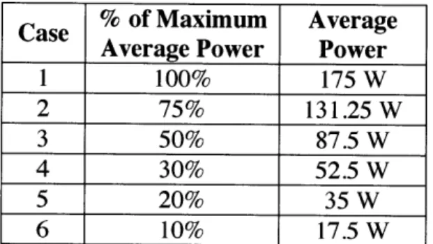
A "CEC efficiency" rating requires measuring the efficiency of the solar micro-inverter

for six different average (over a line cycle) power levels. As described in Chapter 2, these cases are at six different percentages of the maximum average power. Given that the maximum average power is 175W, Table 3.1 shows the different average power levels of interest.

Case % of Maximum Average Average Power Power 1 100% 175 W 2 75% 131.25 W 3 50% 87.5 W 4 30% 52.5 W 5 20% 35 W 6 10% 17.5 W

Table 3.1: Six Different Average Power Levels

For each of these six different average powers, there are three different input voltage levels at which measurements are taken. These are summarized in Table 3.2.

Case Input Voltage 1 25V

2 32.5 V

3 40 V

Table 3.2: Three Different Input Voltage Levels

For each of these three different input voltages, there are fifteen different output voltage levels at which measurements are taken corresponding to fifteen points in the line cycle. These are summarized in Table 3.3.

Case Output Voltage 1 22.6274 V 2 45.2548 V 3 67.8823 V 4 90.5097 V 5 113.137 V 6 135.765 V 7 158.392 V 8 181.019 V 9 203.647 V 10 226.274 V 11 248.902 V 12 271.529 V 13 294.156 V 14 316.784 V 15 339.411 V

3.3: Fifteen Different Output Voltages

The power at a specific output voltage/point cycle, but is directly related to it.

in the cycle is not the average power over a line

Altogether, six different power levels, each with three different input voltage levels, and each with fifteen different output voltages gives two hundred seventy different operating points. Each of these operating points requires four different measurements to be taken: input voltage and current, and output voltage and current. This makes one thousand eighty individual measurements that need to be recorded. Obviously, taking all one thousand eighty readings by hand is cumbersome and tedious, and automation is definitely desirable.

Even after all these one thousand-some measurements are taken, there still needs to be data analysis, such as calculating instantaneous input and output power, computing efficiency for

each operating point, and computing a weight average CEC efficiency rating, as discussed in Chapter 2.

3.2. Automation Algorithm

Figure 3.1 shows a flow diagram of the hardware automation process. The first step is to pick the first average power level. At this power level, the first input voltage is chosen, and then the first output voltage is chosen. Next, the power supplies are set to deliver this input and output voltage. The four multimeters measure and record the input and output voltage and current. As described in Chapter 2, there are associated error bounds for different voltage and current readings on the multimeters depending on range. Thus, error bounds are calculated for these measured nominal voltage and current levels. Input and output power are computed, and through interval analysis, the error bounds on those values are found. Efficiency is calculated next, and again, using interval analysis, the error range on that nominal efficiency is calculated. This completes the measurements for that output voltage. The program repeats for the next output voltage, and iterates through the whole process again until all output voltages have been measured. At this point, the input power supply steps to the next input voltage, and the whole process is repeated for every output voltage. Once all input voltages have been measured, then the next average power level is chosen, and the whole process repeats. Thus, there are three loops. The innermost loop sweeps through all the output voltages, the middle loop sweeps through all the input voltages, and the outermost loop sweeps through all the average power

levels. When the program calculates input and output power as well as efficiency, running figures of this data, with their error bounds, are plotted.

Figure 3-1: Hardware Automation Algorithm

For each operating point, the input voltage and current, output voltage and current, input and output power, and efficiency are recorded with their associated error bounds. After all average power levels have been cycled through, these input and output power values are used to calculate the CEC efficiency of the solar micro-inverter.

The goal of this algorithm is to be applicable not only to the solar micro-inverter, but also to other high frequency power converters. The MATLAB script, which commands this whole

automation process, is easily adapted for other such converters. The only difference would be in removing the CEC efficiency calculation at the end. The solar micro-inverter has six distinct average power levels, three distinct input voltages and fifteen distinct output voltages, but the script can take in any number of average powers, input voltages, and output voltages.

Appendix A documents the MATLAB code written to control this whole master triple loop automation. Special functions were written in order to calculate the error bounds on current and voltage measurements involving the Agilent 34401A look-up tables, which are provided in Appendix B. Other functions that are called in the master loop code, such as opening and closing the port, are presented in Appendix B as well.

3.3. Equipment Setup

A list of equipment used, as described in the Introduction, is reproduced below for

convenience.

Equipment Name Description

HP 6030A Input Power Supply (200V, 17A) HP 6632A Output Power Supply (20V, 5A) HP 6015A Output Power Supply (500V, 5A) Agilent 34401A (x4) Digital Multimeter

Agilent 34330A Current Shunt (30A, 1mV/A) Prologix GPIB-USB Controller

The master loop program commands the power supplies and multimeters through the Prologix GPIB-USB controller, and is compatible on both Mac and Windows platforms. As mentioned in the Introduction, the HP 6015A lacks GPIB control, but has analog programming capabilities. The HP 6632A controls the voltage outputted from the HP 6015A by a 1:10 ratio. Thus, if the HP 6632A outputs 0.1 V, the HP 6015A outputs 10 V. Hooking up the sensing terminals on the power supplies to their output terminals ensures that the voltage commanded is the voltage sourced.

Input current levels reach as high as 14A, which exceeds the current limit ratings on the Agilent 34401A. Thus, the Agilent 34330A current shunt is included to measure the input current. The current shunt attached to the Agilent 34401A gives a voltage reading in a 1mV:1A ratio.

The four multimeters (one which has the current shunt) measure the input and output current and voltages, and it is these measurements that are used to calculate the efficiency. The overall system diagram is shown below in Figure 3.2.

Chapter 4.

System Test and Validation

Verifying the measurement system involves analyzing two separate cases and comparing the results. The first case is the "control," where measurements are taken and recorded by hand. The second case is the "automation," which takes the same measurements but uses the automated system. The test board used is essentially two power resistors, one connected to the input voltage supply, and the other connected to the output voltage supply. Figure 4.1 shows the basic topology of the test board.

IIN 'OUT

VIN RIN ROUT +VOUT

Figure 4-1: Resistor Test Board Topology

The point of the test board is to operate it at points of interest in the micro-inverter topology. Thus, different values were chosen for Rin and Rou, depending on the currents needed. The current levels were chosen to span the complete range of current for the micro-inverter (i.e. from ~50mA to 15A for input current, and ~10mA to 2A for output current). The voltage levels chosen for Vi and V,11 spanned the range of voltages on input and output of the micro-inverter as

well. Given these ranges on current and voltage, three resistors were chosen for Ri. and Rou. Their resistance and current limits are summarized in Table 4.1.

Resistor Resistance Current Limit

A 1.6 Q 22A

B 1.435 kQ 0.54A

C 2.87 k 0.38A

Table 4.1: Resistor Values and Limits for Test Board

A complete listing of all the possible operating points of interest for the micro-inverter is

included in Appendix C.

After verification of the measurement system, sample test data taken from manual measurements of the input and output voltages and currents is processed by the measurement system in order to verify the working state of the CEC efficiency calculation.

4.1. Control Measurements

The control measurements looked at different voltage and current pairs, chosen because they were boundary points. That is, the nominal input voltage was either 25V or 40V, and the nominal output voltage was either 29V or 340V. Using different resistors for the same input and output voltages provides variety in the power level.

Resistor A

Vi. = 25 V Ii. = 15.625 A Pi, = 390.625 W

Resistor B

Vin= 25 V In, =0.0174 A Pin= 0.435 W

Vin= 40 V I 0= 0.0278 A Pin= 1.112 W

Vout =29 V out =0.2567 A Pout = 7.444 W

Vout = 340 V Iot =0.0206 A Pout = 7.004 W

Resistor C

Vi= 40 V In= 0.0139 A Pi= 0.556 W

Vou, =29 V Iou= 0.0103 A Pout =0.299 W

Vou =340 V lout =0.1183 A Pou= 40.222 W

Table 4.2: Control Operating Points

Measurements were taken by manually adjusting the power supplies to the correct voltage, and then manually reading the measurements off the multimeters. The results are shown in Table 4.3.

Resistor A

Vin= 24.8139 V Iin = 15.6690 A Pin = 388.809 W

Resistor B

Vin= 24.9964 V Iin =0.0184 A Pin= 0.4599 W

Vin = 39.9488 V Iin= 0.0295 A Pin = 1.1785 W

Vout = 29.8312 V 'out = 22.4476 mA Pout =0.6696 W Vout = 340.312 V 'out = 256.679 mA Pout = 87.3509 W

Resistor C

Vi =39.9502 V Iin = 0.0152 A Pin= 0.6072 W

Vout =29.8972 V lout 11.42676 mA Pout = 0.3416 W Vout 339.4113 V lout =130.152 mA Pout = 44.1751 W

4.2. Automated Measurements

The automated measurements were taken for the same ranges that the micro-inverter operates. Two distinct tests were run. The first went through the full range of input and output voltages of interest, and the second went through the full range of input currents of interest. This second test was performed because the current shunt limits the input current to be above 50mA in order to still remain measureable. Thus, the second test sets the input current across its full range.

4.2.1.

Test 1: Sweeping All Possible Voltages

The first automated test measures the full voltage ranges on input and output side of the micro-inverter. These values are shown below.

Vin vout 25 V 22.6274 V 32.5 V 45.2548 V 40 V 67.8823 V 113.1371 V 135.7645 V 158.3919 V 181.0193 V 203.6468 V 226.2742 V 248.9016 V 271.5290 V 294.1564 V 316.7838 V 339.4113 V

Table 4.4: Operating Voltages for Automated Test 1

The same resistor test board was used for the automated test, with Ri = 2.87 kQ and Rrnn

= 1.435 kW. The input and output voltage, current, and power are shown in the next eight figures. Error bars have been added to the figures to show the uncertainty in the measurement. For each current and voltage pair, the automated system takes two of the same measurements. The full list of data is available in Appendix D.1.

The automated measurement system also plots efficiency and associated error bars, but since the resistor test board has input completely independent from the output, the calculation of efficiency here is meaningless and is omitted.

Input Voltage Measurement

20 40 60 80 100

Sample Number

Figure 4-2: Test 1 Input Voltage Measurement

The error bars on the figure are so small that they are not easily noticeable. Figure 4-3 shows a zoomed in version of the Test 1 input voltage measurement.

Input Vo tage Measurement

32 34 36 38 40 42 44 Sample Number

Figure 4-3: Test 1 Input Voltage Measurement Zoomed in

32.53 32.525 32.52 32.515 32.51 .35 _g32.505 32.5 32.495 32.49 ... . . ...

mmomm-Input Current Measurement 0.03 0.025 ... . .... ... ... 0.02 . . . . Z a) S0.015... .. 0. 1. .. ..

a.

Figure 4-4: Test 1 Input Current Measurement

The input current measurements seem unstable, but that is due to the fact that the shunt just cannot measure such small current values. The lowest the shunt can read accurately is around 50mA, which accounts for the wide swings in input current. This is not a big problem because the majority of the input currents of interest are at currents significantly higher than

Output Voltage Measurement

20 40 60 80

Sample Number

Figure 4-5: Test 1 Output Voltage Measurement

350 300 250 200 150 100 50 100

Output Current Measurement

20 40 60 80

Sample Number

Figure 4-6: Test 1 Output Current Measurement

0.35 0.3 0.25 0.2 0.15 0.1 0.05 0 100

Input Power Calculatin 1.4 0 26 0.4 .. .. . .... .. . . 0 0 20 40 60 80 100 Sample Number

Figure 4-7: Test 1 Input Power Calculation

The input power varies wildly because the input current varies wildly. Again, this is not a problem because the solar micro-inverter will operate at power levels much higher than 2W.

... ...

pmPp"Mv-90 80 70 60 50 0 a.

'40

Output Power Calculation

0 20 40 60 80

Sample Number

Figure 4-8: Test 1 Output Power Calculation

The maximum uncertainty for each parameter is shown in Table 4.5.

Parameter Maximum

Uncertainty

input voltage 0.004 V

input current 1.7762e-4 A

output voltage 0.0438 V output current 6.1368e-4 A

input power 0.0072 W output power 0.2198 W

Table 4.5: Maximum Uncertainty for Automated Measurements Test 1

The uncertainty on output power may seem high, but considering that this error occurs at the maximum output power calculated, which is around 90W, this uncertainty of 0.2198 is not particularly troublesome.

4.2.2.

Test

2:

Sweeping All Possible Input Currents

Previous automated measurements for input current have been focused on currents in a range that cannot be measured, given the limitation of the current shunt. Thus this second automated test shows the measurement system operating at input current levels at which the solar micro-inverter would be operating. A list of the operating input currents is shown below.

Associated

Input Voltage Input Current

I V 0.625 A 5 V 3.125 A 1OV 6.25 A 15 V 9.375 A 20 V 12.5 A 25 V 15.625 A

Table 4.6: Operating Input Currents and Associated Input Voltage, for Ri. = 1.6Q

The input resistance is 1.6Q, which allows for the current to span from approximately 1A to 16A. The following three figures show plots of the input voltage, input current, and input power. Error bars have been added to the figures to show the uncertainty in the measurement.

For each current and voltage pair, the automated system takes two of the same measurements. The full list of data is available in Appendix D.2.

Input Voltage Measurement

20

-.

0

-...

Figure 4-9: Test 2 Input Voltage Measurements

Input Current Measurement I I

7.

Figure 4-10: Test 2 Input Current Measurements 14 12 10

-.

.

.

.

.

.

.

.

.

.

..

.

.

-.

.

.

.

.

..

.

.

Input Power Calculatin

2 4 6 8 10 12 14

Sample Number

Figure 4-11: Test 2 Input Power Calculations

Parameter Maximum

Uncertainty

Input Voltage 0.0029 V

Input Current 0.0936 A

Input Power 2.3042 W

Table 4.7: Maximum Uncertainty for Automated Measurements Test 2

The input power has a maximum uncertainty of 2.3042W, but this occurs at the maximum input power of around 366 W, so relatively speaking, this is acceptable.

400 350 300 250 200 150 100 50 0

From the measurements presented in the automated system provides measurements that are taken manually. The 50mA minimum on the measurement system, but it is possible to just not u not exceed 3A.

previous two as good as, if input current

se the current

sections, it is clear that the not better, than measurements provides a limitation on the shunt if input current values do

4.3. Solar Micro-Inverter Test Data Analysis

Now that the measurement setup proves to be a reliable system, some sample test data from the solar micro-inverter was acquired to run the code on. Unfortunately, the test data has some serious flaws. First, the test data was taken with a different set of multimeters than the Agilent 34401A that the measurement code was written for. Second, there are an uneven number of input voltage and output voltage pairs for each average power level. Third, only five of the six power levels were swept through. Thus, analyzing this test data with the CEC efficiency calculator part of the measurement code will not provide exactly the same results as those that were manually calculated, but it does provide a nearest answer approximation.

Table 4.8 shows the test data for the solar micro-inverter. The code for analyzing this data, which basically is only the CEC efficiency calculation part of the automation code, is included in Appendix E.

% Average Input Input Current Output Voltage Output Power Voltage [V] [A] [V] Current [A]

100 34 9.74 333.66 0.919 100 34 8.79 314.69 0.879 100 34 5.41 240.53 0.7 100 34 1.65 130 0.383 100 25 7.13 240.53 0.687 100 25 2.22 130.26 0.385 75 34 7.63 333.54 0.725 75 34 6.86 314.56 0.689 75 34 4.14 240.42 0.538 75 34 1.21 130.18 0.276 75 25 11.2 333.58 0.788 75 25 9.39 314.57 0.703 75 25 5.6 240.43 0.542 75 25 1.67 130.19 0.289 50 34 5.46 333.39 0.519 50 34 4.85 314.42 0.487 50 34 2.82 240.3 0.363 50 34 0.663 130.09 0.14 50 25 8.13 333.44 0.578 50 25 6.89 314.44 0.517 50 25 3.93 240.32 0.38 50 25 1.01 130.11 0.169 30 34 3.45 333.27 0.321 30 34 2.97 314.28 0.291 30 34 1.46 240.19 0.177 30 34 0.646 130.08 0.128 30 25 5.66 333.33 0.4 30 25 4.71 314.33 0.351 30 25 2.42 240.22 0.229 30 25 0.572 130.47 0.0833

The next six plots show these measurements and the input and output power and efficiency calculations with their associated error bars.

Yin with Error Bars

26

26

Sarple Number

Figure 4-12: Test Data Input Voltage Measurement

61

I I I I I p

lin with Error Bars

10

I-61[-.

I 5 10 15 20 25 30

Sample Number

Vout with Error Bars

5 10 15 20 25 30 35

Sample Number

Figure 4-14: Test Data Output Voltage Measurement

63 350 300 250 200 150 100 ... mm ooy ....

a-lout with Error Bars 0.6 . 0.5

I

Figure 4-15: Test Data Output Current Measurement

64 0.7 I I I

...

Input and Outpout Power with Error Bars 350 r ... ...

L

UPjut

Power

50

.

Figure 4-16: Test Data Input and Output Power Calculations

300 250

V

Efficiency with Error Bars

5 10 15 20 25 30 35

Sample Number

Figure 4-17: Test Data Efficiency Calculations

It is now quite easy to see that the efficiency calculation with error bars is functional. The next calculation of interest is the CEC efficiency. Table 4.9 shows the trapezoidal integration of the efficiencies for each average power level.

1 0.95 0.9 0.85 0.8 0.75