Low Speed Sensorless Control of Non-Salient Poles Multiphase PMSM

Science Arts & Métiers (SAM)

is an open access repository that collects the work of Arts et Métiers Institute of Technology researchers and makes it freely available over the web where possible.

This is an author-deposited version published in: https://sam.ensam.eu Handle ID: .http://hdl.handle.net/10985/15498

To cite this version :

Diana Angelica TORRES GUZMAN, Ngac Ky NGUYEN, Mohamed TRABELSI, Eric SEMAIL -Low Speed Sensorless Control of Non-Salient Poles Multiphase PMSM - In: The 20th IEEE International Conference on Industrial Technology (ICIT 2019), Australie, 2018-02-14 - IEEE International Conference on Industrial Technology (ICIT 2019) - 2019

Any correspondence concerning this service should be sent to the repository Administrator : [email protected]

Science Arts & Métiers (SAM)

is an open access repository that collects the work of Arts et Métiers ParisTech researchers and makes it freely available over the web where possible.

This is an author-deposited version published in: https://sam.ensam.eu Handle ID: .http://hdl.handle.net/null

To cite this version :

Diana Angelica TORRES GUZMAN, Ngac Ky NGUYEN, Mohamed TRABELSI, Eric SEMAIL -Low Speed Sensorless Control of Non-Salient Poles Multiphase PMSM - In: The 20th IEEE International Conference on Industrial Technology (ICIT 2019), Australie, 2018-02-14 - IEEE International Conference on Industrial Technology (ICIT 2019) - 2019

Any correspondence concerning this service should be sent to the repository Administrator : [email protected]

1

Low Speed Sensorless Control of Non-Salient

Poles Multiphase PMSM

Diana Angelica Torres Guzman, Ngac Ky Nguyen, IEEE member, Mohammed Trablesi, IEEE member, Eric Semail, IEEE member

Univ. Lille, Centrale Lille, Arts et Metiers ParisTech, HEI, EA 2697 - L2EP - Laboratoire d’Electrotechnique et d’Electronique de Puissance, F-59000 Lille, France

E-mail: {diana_angelica.torres.guzman; ngacky.nguyen; [email protected] }

Abstract –This article presents the development of an algorithm which can be used at standstill and low speed for sensorless control of a five-phase Permanent Manget Synchronous Machines (PMSM) with non-salient poles. The estimation method is based on the machine’s torque. Two different strategies are investigated for the proposed method. The first one uses the torque measurement and the second one uses the estimated torque from the measured currents. Results for the implementation of both strategies are presented and analysed, together with possible improvements to explore.

Keywords— Initial rotor position, multiphase drive, sensorless control, surface permanent magnet synchronous motor (SPMSM), rotor position estimation, non-salient pole machines

I. INTRODUCTION

M

ULTIPHASE machines have become an interesting research topic in electrical engineering for sustainable development due to their ample range of applications and multiple advantages when compared to classic three-phase machines. Some of these advantages include smaller power electronic components dimensioning (the power is split into more than three phases) and fault tolerance capability [1]. The automotive application is moving to a tendency of low voltage for user safety with more embedded power on board. Needing more compact and lighter propulsive systems leads to a necessity to integrate power electronics inside the machine.

One of the challenges associated to the integrated motor drives is the elimination of the rotor position sensor, i.e. the electromechanical sensors which are commonly used to obtain the accurate rotor position information for high-performance vector control of PMSM drives. The use of these sensors for a machine integration not only increases the cost, size, weight, and wiring complexity, but also reduces the reliability of the drive because of thermal conditions. Moreover, using width-band gap components such as GaN lead to a significant electromagnetic compatibility phenomena induced to the sensor position if they are placed closely.

In order to achieve sensorless control for multiphase drives at low and zero speed, many challenges have been identified. They are:

 Difficult or no back-EMF observability at low speeds,  The absence (or very low) of reluctance effect in

non-salient machines,

 The problem associated with the multiphase drives which imply more complicated models and parameters,

 The question of classical methods adaptability for multiphase drives.

Commonly, in order to perform sensorless control in PMSMs, model-based methods are used [2]. When the rotor is not moving, or it is moving at low speed, this information is no longer available (or is of low quality) and the model-based methods do not work well [3]. This is the reason why specialized methods for low speed and standstill were conceived.

Amongst the main different low speed and standstill methods for a PMSM found on the literature, such as in [3], [2]-[4], a broad classification could be made, distinguishing four different types: high frequency (HF) signal injection presented in [2],[3],[5-7] (including sinusoidal wave, rotating voltage, square wave injection and pulse injection methods), inductance variation (based on the INFORM method) [8], Pulse Width Modulation (PWM)-based methods [6] and the Magnetic Anisotropy Method (MAM) [4].

The common feature of these methods is the inclusion of a perturbation by injecting a HF signal or pulses into the machine through the inverter, in order to recover the rotor position thanks to the interaction of this perturbation with the saliency of the PMSM. This technique has a number of drawbacks in the practical implementation, such as audible noises and increasing the torque ripple [9]. Furthermore, it can only be effectively used when the aforementioned saliencies are significant enough as to cause a difference in d-q axes impedances of the synchronous rotor frame of the decoupled primary machine.

The particularity of non-salient pole machines is that they have very similar impedances in the d-q axes in the decoupled frame. This implies that there is no position-dependent component of the measured impedance at any point. This presents itself as an issue for most signal injection methods which depend on this property.

Other signal injection methods, such as the one presented in [3], may present the issue that the output does not yield directly the actual position of the rotor, but the position of an ambiguously set estimated angle. This angle will then be made to converge to the actual rotor position by different techniques such as lookup tables in the control-loops, and/or starting strategies which may indeed need to get the machine to a certain speed before beginning to perform closed-loop sensorless control.

2 So far, there is little evidence in the literature for

sensorless position estimation methods being tested for a non-salient pole PMSM. For this reason, the issues related to the adaption and practical implementation of such a method in the multiphase machine, have not been properly encountered, described and addressed. It is nonetheless possible to assume that many of the challenges inherent to position detection methods based on saliency for multiphase PMSM may be transposable to the non-saliency based case.

Based on the previous analysis, it can be argued that it is not possible to estimate the actual rotor position of a PMSM having no salient poles with an injection method without including a strategy to minimize the error between the estimated rotational reference frame and the actual rotor frame. As it is proven in [10], this convergence from an estimated reference frame into the actual rotor frame is possible to achieve, even without signal injection.

Based on this idea, an original method is proposed. This method uses the measured machine phase currents. A torque optimization algorithm based on the machine model is then defined to find the rotor angle. The proposal is similar to the one used in “Recursive Least Square” or “Least mean Square” (LMS) methods [11].

The paper is organized as follows: the machine model is explained in section II. The methodology is detailed in Section III. Section IV will present the simulated and practical results obtained, together with a brief analysis and a discussion on potential work ahead. Conclusions are presented in Section V.

II. FIVE PHASE PMSM MACHINE MODEL WITH NO SALIENT POLES

An expression for the five-phase PMSM stator voltages can be expressed as in equation (1).

 

v R i

       

d i e dt

  L  ₍₁₎

where : [v]: 5-dimension voltage vector [i]: 5-dimension current vector [e]: 5-dimension back-EMF vector [L]: 5-dimension inductance matrix R: stator phase resistance

All electrical values in the natural frame can be expressed as a combination of the projections of these values into a ‘decoupled’ frame, with the use of the Concordia transformation. In this way, one five-phase machine can be decoupled into two fictitious independent two-phase machines defined by the projection in the planes (xα, xβ) and

(xx, xy), and a fictitious one-dimensional homopolar machine

defined by the projection in the line eigenvector xh [12].

Each coordinate of a magnitude in the ‘eigenspace’ corresponds to a harmonic group with the real magnitude of the machine in the natural frame. This means that each fictitious machine will have a unique interaction with specific harmonics of the machine’s natural frequency. The final result is the added effect of each independent fictitious machine. For a five-phase machine, the harmonics corresponding to each fictitious machine are described in Table I.

TABLE I.HARMONICS ASSOCIATED TO DECOUPLED MACHINES [12]

Fictitious Machine Decoupled frame

Families of harmonics (odd only) Main Machine α-β 1, 9, 11, …, 5v ± 4, Secondary machine x-y 3, 7, 13, …, 5v±2, Homopolar machine h 5, 15,…, 5v

In order to obtain a model that is suitable for control purposes, a ‘Park’ transformation (2) is applied to rotate the frame, in order to deal with constant electric values in the d-q frame. Thus, for the Main Machine (MM), the Park transformation is done for θ, and for the Secondary Machine (SM) for 3θ (as it has been established that the fictitious secondary machine rotates at three times the speed of the main machine and in the opposite direction). The homopolar machine, being one-dimensional and perpendicular to the others, does not considered in this work because of a wye-connection:

- for the MM (the 1st _harmonics)

 

1 cos( ) sin( ) sin( ) cos( ) p p p R p          _{  }    

- for the SM (the 3rd harmonics)

 

3 cos(3 ) sin(3 ) sin(3 ) cos(3 3 ) p p p R p          _{  }   _   (2)

The final result is the frame voltages used in vector control. If using, for example, the Concordia transform, the equations which describe the primary and secondary machine are (3) – (4) and (5) - (6) respectively.

In these equations, id,q, ix,y, Vd,q and Vx,y represent the

currents and voltages of the rotor frame of the primary and secondary machines, R and L are the phase resistance and inductance in the decoupled frames, is the magnetic flux of the permanent magnets, p the number of pole pair, ωe the

electrical angular speed, and Tm, Ts the torque of the primary

and secondary machine respectively. Electrical equations of the MM:

5 2 0 d d e q d q e d q q _e V R sL L i V L R sL i         _      _{    }    _{    }    _{    }   (3) Electromagnetic torque of the MM:





5 2

m q d q d q

T  p_ i L L i i _{ (4)}

Electrical equations of the SM:

x e y x e y y y x x x y R sL L V i L R sL V i                        (5)

Electromagnetic torque of the SM:





5 2

s y x y x y

T  p_ i L L i i _{ (6)}

The final torque component will be the addition of the outputs on the main and secondary machine T=Tm+Ts.

3 III. ESTIMATION METHOD FOR SENSORLESS

CONTROL OF A 5-PHASE PMSM

Two strategies based on the torque optimization algorithm are investigated. In the first one the torque measurement is obtained from the sensor available on the electric drive system. The second strategy aims to eliminate the need for this torque sensor. When the torque sensor is removed, an estimated torque derived from the measured currents is used instead.

The idea consists on the possibility of applying a simple optimization technique to the machine torque equation, which allows finding the position  that would maximize current _est iq. The solution to this problem helps guarantee that the

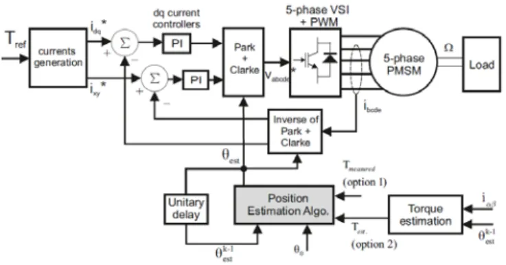
optimal position value _{est opt-} will be equal to the actual rotor position _actual as will be explained in this session. The complete setup for this method and the control of the machine is seen in Fig. 1.

For simplicity, the methodology presented in this section is constructed under the assumption that the total torque is produced by the main machine (T=Tm), i.e sinusoidal

back-EMF and thus there is no third harmonic injection (Ts=0). In

the case where the secondary machine torque is included (Ts≠0), the method would need to be extended.

A. Algorithm Construction

From equation (4), it can be seen that, in the general case for a synchronous machine in steady state, the torque component can be expressed in terms of current iq, and an

effect due to the machine’s saliencies:



L_dL i i_q



_{d q}. For a machine with no saliencies, equation (4) is further simplified as in (7).

5

2 q

T  p i ₍₇₎

If T T _measured, current component i_q can be expressed as follows: 2 5 measured q T i p   (8)

Based on the Park transform (2), it is possible to express

q

i in terms of the currents in the stationary decoupled frame iα,β, as in (9).









sin cos

q actual actual

i  i p i p (9)

When there is no position sensor, the measured position

actual

 needs to be replaced with an estimation . If the _est estimated position is used in equation (9), the Park transformation will yield an estimated value of i , defined as _q

q est

i_ in equation (10).









sin cos

q est est est

i  i p i p (10)

From (9) and (10), it is possible to deduce that, when the angle estimation is equal to the actual angle_est_actual, the current will be equal to the actualvalue of theestimated

Fig. 1 : Torque control of the 5-phase PMSM.

current iq est



actual



iq, and it will assume its maximum

possible value. Therefore, it can be said that when θest →

θactual, equation (11) becomes true.









2 sin cos 5 measured est est T i p i p p       (11)

Based on this methodology, it possible to design an algorithm which would be used to minimize the error ε, as proposed in the following optimization problem (12).

 

min( )    













2 sin cos 5 measured est est T i p i p p          0 pest2 (12) An algorithm is therefore developed in order to solve this 1-D minimization problem in real time. The method consists of five global steps as shown in Fig. 2.

Fig. 2 : Position estimation method

1) Step 1 : Signal acquisition and conditioning

Signals iα iβ and torque are recovered and filtered. Since

operation rates of the algorithm are slower than the sampling frequency, rate converters are utilized.

2) Step 2: Optimization algorithm

After acquisition of the signals, the optimization algorithm is executed. This algorithm is illustrated in Fig. 3 and described in numerals a) to f).

a) Establishing step and maximum iterations based on speed

The speed reference is used in order to define the coefficients that will determine the ‘step’ value. The step is the maximum angle variation possible for each iteration. A maximum number of iterations is also defined taking into account the algorithm execution time vs. minimum desired error. A large number of iterations, i.e smaller error, makes the algorithm slower (leading to delay-related errors). A compromise between these two things must be found.

4

Fig. 3 : Optimization Algorithm

b) Initial point and Polarity detection

An initial point  needs to be chosen to start the ₀ iterations. If this is done for the first time, the initial point is chosen randomly. Else, this point will correspond to the value calculated in the previous iteration. That is, for a given moment k , the initial point will be k 1

est

  _{. From this point, it is}

convenient to use a polarity detection method and many exist in the literature [13]. In this case, the error equation in (13) is evaluated for the input estimated angle k1

est

  _{. Then, the same}

error is evaluated for the opposite side k 1 est

  _{ . Whichever}  yields the minimum error will be chosen as the new estimation to begin the iterative optimization process.

 

 



1 1



2 _{sin cos} 5 k k measured est est T i i p   _{  }   _    (13) c) Error initialization: 1

 is calculated with the chosen k 1 est

  _. 2

 will be initialized equal to  for the first iteration. ₁

 

 



1 1



1 2 2 sin cos 5 k k measured est est T i i p    _ _{  }   _    (14) d) Optimization loop:

The loop calculates the solution to the problem described in (14), performing as follows:

 Take the last angle estimation and defined step to form a vector ‘x’, as described in (15) :

1 0 1 0 1 2 1 2 , , ,...., k est k n est step x step x x n step x x x step n x                          (15)

It should be noticed that we have 2n points for each iteration as shown in Fig. 3.

 Calculate  for each_k x_k. Chose the angle that yields the lowest error, which will be . Then, call it*  , ₂ as : 2 *

 If  <₂  , ₁

- Readjust step (the step gets smaller as the calculated error gets smaller values).

- Make , k1 _*

est x

  _

- Repeat numerals 1. to 3.

 If  >₂  , or a maximum number of iterations is ₁ reached, exit loop.

e) Best angle pick:

It is possible to compare the results of *x for the two last iterations with the original 1

est

 _{and pick the best. This will be}

the output.

f) Torque verification:

In sensorless operation an additional step is performed in order to verify that the estimated torque corresponds or is ‘close’ to the reference. A lower value is sometimes observed, due perhaps to a lag or delay caused by filters and computation time. If needed, a small angle is added to the exit of the algorithm.

3) Step 3: Calculated position re-injection

Results are fed back into the algorithm to serve as an initial value to perform next calculation.

4) Step 4: Torque estimation (optional)

This step is performed when the torque measurement is replaced by an estimation. A separate block calculates the torque based on the estimated angle output.

5) Step 5 - Closed loop control

The 2 modulus is calculated in order to get the estimation used for closed loop sensorless control. This estimation is used to perform all necessary calculations in the machine model.

IV. SIMULATION AND EXPERIMENTAL RESULTS The machine is a five-phase non-salient pole machine with 7 pole pairs. The main parameters of the machine are listed in Table II.

TABLE II.PARAMETERS OF THE MACHINE USED IN SIMULATION AND IN PRACTICAL IMPLEMENTATION

Parameter Name Value

Phase resistance R 0.0091Ω Phase inductance L 0.9x10-3_H

Mutual inductance M1 0.02x10-3H

Sec. Mutual Inductance M2 -0.01x10-3H

5

Inertia J 0.0052 kg.m2

Voltage DC V 48V

Base-Maximum speed ωB 1500-18000 rpm

The sampling time for these simulations is 400 μs, in order to match the minimum possible computation time of the dSPACE platform used in the controller implementation.

When the strategy including torque measurement is simulated, the algorithm can be run standalone and with no special considerations at the startup. When using a torque estimation, sensorless operation begins at 0.5 s.

A. Simulation Results

1) Torque control with torque “measurement”

The control scheme shown in Fig. 1 was simulated in Matlab/Simulink. The torque control is considered (Tref = 15

Nm) and the speed is imposed by the load. Figures 4-7 show the simulation results for angle estimation vs. the actual position, estimation error in degrees, torque and phase currents respectively. The torque is “measured” by taking the real position, i.e real rotor flux multiplying to the stator currents.

The simulation includes startup and steady-state response for an example with a rotor speed of 10 rpm (0,67 % of the base speed). It can be observed that correct closed-loop control can be achieved for low speed applications, with an error of about 1-3 electrical degrees.

Fig. 4 : Simulation - Actual vs. estimated angles (torque measurement).

Fig. 5 : Simulation - Angle error (with torque measurement).

Fig. 6 : Closed loop Torque response (with torque measurement).

Fig. 7 : Currents in the natural frame (with torque measurement).

Fig. 8 : Simulation - Actual (red) vs. estimated (blue) angles (sensorless from 0.5s)

Fig. 9 : Simulation – Angle error (sensorless from 0.5s)

2) Torque control with torque estimation

Fig. 8 and Fig. 9 show the closed-loop angle and angle estimation for a sensorless control at 10 rpm.

A simulation is made with Matlab/Simulink with a torque estimation instead of the torque “measurement”. It was not possible to startup the machine without initial conditions. Therefore, for the first 0.5 s, the angle measurement is used. In this simulation, 0.5s is chosen to ensure a stability and make sure the convergence of the algorithm. This value depend the dynamic of the close loop control of the drive.

B. Experimental test

The experimental setup is shown in Fig. 10 where the 5-phase is driven by a 3-5-phase industrial Parvex Drive. The speed is imposed at 10 rpm by the latter and the 5-phase is performed in torque control. A position sensor is used to validate the angle estimation. A torque sensor is also used.

Fig. 11 and Fig. 12 show the estimated angle vs. measured one and the error between them respectively. Fig. 13 and Fig. 14 show current and torque measurement. The 5-phase motor is run at low speed 10 [rpm] by the 3-5-phase Parvex Drive. We can see that the estimated angle is followed the measure one. The error varies from 10° to -8°electric degrees. Each revolution changing due to the “mod” function used in Matlab, the error is equal 2π because of a delay induced by the filter used in algorithm.

6

Fig. 10 : Setup for testing rotor position estimation on a five-phase PMSM.

Fig. 11 : Experimental result - Actual vs. estimated angle. Closed loop control with torque measurement at 10 rpm.

Fig. 12 : Experimental result - Electrical angle error in degrees. Closed loop control with torque measurement at 10 rpm.

Fig. 13 : Experimental result - Measured torque (filtered) vs. Reference. Closed loop control with torque measurement at 10 rpm.

Fig. 14 : Experimental result - Phase currents. Closed loop control with torque measurement at 10 rpm.

Fig. 13 reports the torque measurement and the reference one. Fig. 14 shows the machine phase currents. We can see that even at very low speed (10 rpm), the machine torque is closed to the requirement. This result is promising and can be improved.

V. CONCLUSIONS

This article presented a comprehensive methodology to design and implement a sensorless control of a five phase PMSM with non-salient poles. It was concluded that, given the condition that there is a required torque, the angle can be correctly estimated, with an acceptable steady state error of maximum 4-5 degrees at low speeds. Using torque measurement, the method allows closed-loop control with a maximum error of about 10 °at 10 RPM. There aren’t yet clear results for closed-loop response in the practical implementation when the torque is estimated rather than measured. Further work is needed to achieve sensorless implementation without torque sensing. Although the method shows promising results, a certain amount of issues remain to be improved such as the robustness, the sensitivity to parameters variation and the execution rate between the estimation bloc and others.

REFERENCES

[1] E. Levi, "Advances in Converter Control and Innovative Exploitation of Additional Degrees of Freedom for Multiphase Machines," IEEE

Transactions on Industrial Electronics, vol. 63, pp. 433-448, 2016.

[2] M. Ramezani and O. Ojo, "The Modeling and Position-Sensorless Estimation Technique for A Nine-Phase Interior Permanent-Magnet Machine Using High-Frequency Injections," IEEE Transactions on

Industry Applications, vol. 52, pp. 1555-1565, 2016.

[3] Z. Yue, Z. Zhe, M. Cong, W. Qiao, and Q. Liyan, "Sensorless control of surface-mounted permanent-magnet synchronous machines for low-speed operation based on high-frequency square-wave voltage injection," in 2013 IEEE Industry Applications Society Annual

Meeting, 2013, pp. 1-8.

[4] J. Persson, M. Markovic, and Y. Perriard, "A new standstill position detection technique for non-salient PMSM's using the magnetic anisotropy method (MAM)," in Fourtieth IAS Annual Meeting.

Conference Record of the 2005 Industry Applications Conference, 2005., 2005, pp. 238-244 Vol. 1.

[5] F. Briz and M. Degner, "Rotor Position Estimation - A Review of High-Frequency Methods," IEEE Industrial Electronics Magazine, vol. 5, pp. 24-36, 2011.

[6] C. S. Staines, G. M. Asher, and K. J. Bradley, "A periodic burst injection method for deriving rotor position in saturated cage-salient induction motors without a shaft encoder," IEEE Transactions on

Industry Applications, vol. 35, pp. 851-858, 1999.

[7] R. Antonello, F. Tinazzi, and M. Zigliotto, "Benefits of Direct Phase Voltage Measurement in the Rotor Initial Position Detection for Permanent-Magnet Motor Drives," IEEE Transactions on Industrial

Electronics, vol. 62, pp. 6719-6726, 2015.

[8] M. Schroedl, "Sensorless control of AC machines at low speed and standstill based on the "INFORM" method," in IAS '96. Conference

Record of the 1996 IEEE Industry Applications Conference Thirty-First IAS Annual Meeting, 1996, pp. 270-277 vol.1.

[9] O. Benjak and D. Gerling, "Review of position estimation methods for PMSM drives without a position sensor, part III: Methods based on saliency and signal injection," in 2010 International Conference on

Electrical Machines and Systems, 2010, pp. 873-878.

[10] H. Chen, C. Hsu, and D. Chang, "Position sensorless control for five-phase permanent-magnet synchronous motors," in 2014 IEEE/ASME

International Conference on Advanced Intelligent Mechatronics, 2014,

pp. 794-799.

[11] G. Wang, T. Li, G. Zhang, X. Gui, and D. Xu, "Position Estimation Error Reduction Using Recursive-Least-Square Adaptive Filter for Model-Based Sensorless Interior Permanent-Magnet Synchronous Motor Drives," IEEE Transactions on Industrial Electronics, vol. 61, pp. 5115-5125, 2014.

[12] E. Semail, A. Bouscayrol, and J. P. Hautier, "Vectorial formalism for analysis and design of polyphase synchronous machines," European

Physical Journal-Applied Physics, vol. 22, pp. 207-220, Jun 2003.

[13] S. Mariéthoz and M. Morari, "Multisampled model predictive control of inverter systems: A solution to obtain high dynamic performance and low distortion," in 2012 IEEE Energy Conversion Congress and