Adaptive Spatiotemporal Node Selection in Dynamic Networks

(1)

Adaptive Spatiotemporal Node Selection in Dynamic Networks

The MIT Faculty has made this article openly available.

Please share

how this access benefits you. Your story matters.

Citation

Hari, Pradip et al. “Adaptive Spatiotemporal Node Selection

in Dynamic Networks.” Proceedings of the 19th International

Conference on Parallel Architectures and Compilation Techniques,

September 11-15, Vienna, Austria: ACM, 2010. 227-236.

As Published

http://dx.doi.org/10.1145/1854273.1854304

Publisher

Association for Computing Machinery

Version

Author's final manuscript

Citable link

http://hdl.handle.net/1721.1/64736

Terms of Use

Creative Commons Attribution-Noncommercial-Share Alike 3.0

Detailed Terms

http://creativecommons.org/licenses/by-nc-sa/3.0/

(2)

Adaptive Spatiotemporal Node Selection in Dynamic

Networks

Pradip Hari1, John B. P. McCabe1, Jonathan Banafato1, Marcus Henry1, Kevin Ko2, Emmanouil Koukoumidis2, Ulrich Kremer1, Margaret Martonosi2, and Li-Shiuan Peh3

1_{Dept. of Computer Science, Rutgers University,}_{{phari, jomccabe, banafato, marcusah, uli}@rutgers.edu} 2_{Dept. of Electrical Engineering, Princeton University,}_{{kko, ekoukoum, mrm}@princeton.edu}

3_{Dept. of Electrical Engineering and Computer Science, Massachussetts Institute of Technology, peh@csail.mit.edu}

ABSTRACT

Dynamic networks—spontaneous, self-organizing groups of devices—are a promising new computing platform. Writing applications for such networks is a daunting task, however, due to their extreme variability and unpredictability, with many devices having significant resource limitations. Intel-ligent, automated distribution of work across network nodes is needed to get the most out of limited resource budgets.

We propose a novel framework for distributing computa-tions across a dynamic network, in which applicacomputa-tions spec-ify their spatiotemporal properties at a very high level. The underlying system makes node selection decisions to exploit these properties, producing high quality results within a fixed resource budget. A distributed computation is expressed as a semantically parallel loop over a geographic area and time period. Feedback from the application about the quality of node selection decisions is used to guide future decisions, even while the loop is still in progress. This simplifies the process of writing dynamic network applications by allow-ing programmers to focus on the goals of their applications, rather than on the topology and environment of the network. Our framework implementation consists of extensions to the Java language, a compiler for this extended language, and a run-time system that work together to provide a sim-ple, powerful architecture for dynamic network programming. We evaluate our system using 11 Nokia N810 tablet PC de-vices and 14 Neo FreeRunner (Openmoko) smartphones, as well as a simulation environment that models the behavior of up to 500 devices. For three representative applications, we obtain significant improvements in the number of useful results obtained when compared with baseline node selection algorithms: up to 745% (measured), 117% (simulated) for an Amber Alert application; 38% (measured), 142% (simu-lated) for a Bird Tracking application; and 86% (measured), 209% (simulated) for a Crowd Estimation application.

Permission to make digital or hard copies of all or part of this work for personal or classroom use is granted without fee provided that copies are not made or distributed for profit or commercial advantage and that copies bear this notice and the full citation on the first page. To copy otherwise, to republish, to post on servers or to redistribute to lists, requires prior specific permission and/or a fee.

Categories and Subject Descriptors

D.1.3 [Programming Techniques]: Concurrent Program-ming—distributed programming, parallel programming ; D.3.3 [Programming Languages]: Language Constructs and Features—concurrent programming structures; C.2.4 [Computer-Communication Networks]: Distributed Systems—cloud

computing

General Terms

Languages, Performance

Keywords

Spatial programming, spatiotemporal programming, dynamic networks, ad hoc networks, node selection, adaptive schedul-ing, feedback-directed schedulschedul-ing, quality of result, location-awareness, resource-awareness

1. INTRODUCTION

A dynamic network is a set of potentially mobile devices (nodes) in a specific geographic area, which forms sponta-neously rather than being configured in advance. Devices offer services to each other, such as sensing, accelerated com-putation, and data storage. To do so, each device must share its resources (e.g., I/O device access, CPU time, disk space, etc.). One can use such networks for purposes such as traffic monitoring, distributed search and surveillance [25], grassroots launching of new mobile services, and community-based participatory research [3]. Unlike a traditional sensor network, the nodes of a dynamic network may all have dif-ferent owners who seek compensation for the use of their resources. We assume a virtual currency system [15] to in-centivize service provision; units of currency are called “cred-its”. Nodes advertise a price in credits for each service they offer, which they can change in response to demand or re-source scarcity (such as battery charge level). Applications purchase services, and must stay within their budgets. Ex-ploration of pricing policies is beyond the scope of this paper. Time and geography are critical to dynamic network ap-plications. For example, the usefulness of a sensor reading is strongly tied to the time and place at which it is taken, and the cost of a distributed computation will often be depen-dent upon the time allotted for it. If an application had an infinite budget, it could purchase access to the resources of

(3)

all other nodes at all times. Realistically, however, applica-tions must make difficult choices about when and where to spend scarce credits in order to maximize their productivity. Our work builds upon the central observation that dy-namic network applications have spatiotemporal properties that can be exploited to achieve a better overall program outcome. This leads to a novel strategy for expressing and satisfying an application’s node selection needs. We eval-uate our strategy in the context of Sarana, a high-level parallel programming architecture for dynamic networks. The Sarana framework enables applications to express their spatiotemporal properties, which it uses to perform effec-tive, automated node selection and scheduling under a user-specified budget. Properties can be holistic, describing the desired spatial or temporal distribution of selected nodes. They can also be dynamic, describing desired run-time events (computational results or sensor readings), so that Sarana can target devices likely to yield such events. While prior work has mainly focused on issues specific to individual nodes or network links (quality of service), or the network-centric management of resources, our approach is application-centric. The main contributions of this paper are as follows:

Language. Our language employs a parallel loop con-struct to describe distributed computations. Each iteration visits a node and invokes a service. We extend this com-mon paradigm by adding novel abstractions for expressing the spatiotemporal properties of the application, and con-structs by which the application can evaluate the results of a distributed computation and provide dynamic feedback to the system. We chose a language over a library imple-mentation of our new programming abstractions to allow a simpler specification of spatiotemporal properties, and to enable compile-time analyses and future optimizations.

Prototype. Our prototype Sarana implementation con-sists of a compiler, a run-time system, and an adaptive, spacetime-aware scheduler that support and exploit the ab-stractions in our language. Three driver examples with dis-tinct spatiotemporal properties are used to illustrate the ex-pressiveness of the new abstractions: a collaborative image capture and analysis application (Amber Alert), a straight-forward sensing application (Bird Tracking), and a space-and time-dependent image sampling application (Crowd Es-timation). The prototype system is able to deal with differ-ent types of failures, including the unavailability of desired services, a lack of sufficient credits to access available ser-vices, and the unresponsiveness of nodes that agreed to pro-vide a service.

Experiments. We evaluate our prototype using a net-work of 11 Nokia N810 tablet PCs and 14 Neo FreeRunner (Openmoko) smartphones, as well as in simulations involv-ing up to 500 nodes. These demonstrate the feasibility, ef-fectiveness, and scalability of our prototype system. For all three driver applications, we achieve significant improve-ments over non-adaptive scheduling that is not spacetime-aware. For Amber Alert, up to 117% (in simulation) and 745% (in the physical evaluation) more useful images were collected using the same cost budget and a low latency limit. For Bird Tracking, up to 142% (in simulation) and 38% (in the physical evaluation) more useful microphone readings were collected. For Crowd Estimation, up to 209% (in sim-ulation) and 86% (in the physical evaluation) more images were acquired within the same time window.

2. SPATIOTEMPORAL PROPERTIES AND

SAMPLE APPLICATIONS

2.1 Spatiotemporal Properties

Clustering. Desirable events may exhibit spatial and/or temporal locality. For example, if we sample a network of cameras and one camera captures an object of interest, it is likely that other cameras near the first one could provide alternate views of the object. Directing further requests to those nearby cameras is a better use of scarce credits than further random sampling. In spatial clustering (Figure 1(a)), node selection is directed towards promising geographic sub-regions. In temporal clustering (Figure 1(b)), node visits are increased in the immediate aftermath of a positive event.

Dispersal. The presence of one event at a particular time and place may make it unlikely that another desired event would occur nearby. For example, if we access an astro-nomical telescope camera and our image suffers from a local disruption (e.g. solar flare), further readings in the immedi-ate future may be similarly unusable. In spatial dispersal, node selection is directed away from unpromising geographic regions (Figure 1(d)). In temporal dispersal, node visits are discouraged in the immediate aftermath of a negative event. Coverage. An application may need a representative sample of sensor readings over a geographic region or time period. For example, we may want photographs of an area that are guaranteed not to leave any large fraction of the area unobserved. Or, we may want the photographs to form a time series at regular intervals. With spatial coverage (Figure 1(e)), a geographic region is divided into equal-area sectors and each sector is sampled (if possible). With tem-poral coverage (Figure 1(f)), a time period is divided into equal intervals and a sample is taken at each interval (if possible).

Synchronization. An application may need a set of sen-sor readings at the same time or place. For example, we may want roughly simultaneous photographs of an object that is moving or changing somehow, so that the informa-tion in these separate photographs can be correlated. In spatial synchronization, (Figure 1(h)) node selection is di-rected to a specific point (or small subregion) chosen by the system from a larger region specified by the programmer. In temporal synchronization (Figure 1(i)), all node visits are scheduled to occur at one specific time chosen by the system, within the deadline specified by the programmer.

2.2 Sample Applications

Amber Alert (spatiotemporal clustering). Amber Alert is a program run by U.S. law enforcement agencies to find abducted children, particularly during the crucial first few hours after the abduction has been reported. A pilot pro-gram involves sending text messages to participating cell-phone users to watch for public announcements on TV, ra-dio, and roadside billboards. A system such as Sarana im-proves the effectiveness of the search through opportunis-tic and paropportunis-ticipatory sensing. A search request looking for a particular car or person can be injected into a network of cameras, including stationary surveillance, traffic mon-itoring, and security cameras, as well as mobile cameras in smartphones and PDAs. Specialized image understand-ing code that identifies search targets within a photo is in-stalled across the designated search area, allowing efficient in-network image processing. If a search target is identified,

(4)

space space

time

(a) spatial cluster-ing (b) temporal clus-tering space space time (c) spatiotempo-ral clustering (d) spatial disper-sal space space time

(e) spatial cover-age space space time (f) temporal cov-erage space space time (g) spatiotempo-ral coverage space space time (h) spatial syn-chronization space space time

(i) temporal syn-chronization space space time (j) spatiotemporal synchronization

Figure 1: Spacetime patterns that can be expressed in Sarana. Shading indicates spacetime subregions that should be preferred in node selection.

the image is sent to participating smartphone and PDA users near where the image was taken. These users may now con-firm the presence of the target, take further pictures, tag them with additional information, share these pictures with others close by, and alert the appropriate law enforcement authorities. For Amber Alert, an effective scheduling strat-egy is to cluster invocations of a camera service around lo-cations and times at which images of search targets were previously identified.

Bird Tracking (spatial dispersal, weighted events). This application tries to record bird songs in a target area (e.g. a forest) using a network of microphones. If a loud noise is detected by a microphone (e.g., due to logging activities), the likelihood of detecting the sound of a bird is minimal, so node selection should be directed away from noisy areas. Additionally, the size of the excluded space should increase with the volume of the noise.

Crowd Estimation (temporal synchronization, spatial coverage). This application tries to take photos that will be used to estimate the number of people at a large outdoor gathering. All photos should be taken at approximately the same time, to avoid double-counting or undercounting peo-ple in motion. To ensure an accurate count, the cameras should be distributed evenly across the area, and we may have to wait to take photos until such a spatial distribution can be obtained.

3. SOLUTION FRAMEWORK

3.1 Language Constructs

Sarana adds network macroprogramming extensions to the Java programming language (Figure 2). A spatialre-gion is an abstract set of devices offering a specific service in a geographic area. A visit statement is similar to a parallel FORALL loop [12]: loop iterations may be executed in

par-allel on separate nodes of the dynamic network. visit loops do not contain synchronization or data dependences other than those generated by reduction variables [12], which are variables whose values are generated by commutative reduc-tion operareduc-tions. Comparable approaches have been used by other spatial programming systems such as Regiment [18], SpatialViews [20], and Pleiades [13]. However, these systems do not have a notion of adaptive scheduling based on the cost of resources or services. Regiment allows static specification of data flow between geographic regions. SpatialViews sup-ports spatial coverage and allows dynamic specification of geographic regions, but nodes are chosen either exhaustively or randomly within those regions, irrespective of the costs they would impose. Pleiades allows dynamic specification of regions, but the selection of nodes must be done by the programmer; the system does not track costs. In Sarana, the run-time system, not the programmer, selects nodes to visit so as to maximize useful results within the application’s budget. This process can be constrained via optional spec-ifications of the minimum and maximum number of nodes that should be visited. Two key additional language features give the programmer the ability to provide feedback about the outcome of loop iterations and guidance about achieving positive outcomes.

First, a loop body may contain report statements, which signal user-defined events. Events describe the outcome of individual loop iterations; typically, raising an event will correspond to the determination that an iteration produced useful results. An optional floating-point value between zero and one indicates the weight of the event, with 1.0 (the de-fault) being the strongest possible feedback. For example, Amber Alert defines an event called GOODPIC that is re-ported when a photo matches the search target (e.g., a miss-ing child).

(5)

SRDecl ::= spatialregion space = service @ region ;

ReportStmt ::= report event [= weight];

VisitStmt ::= visit Range Member Timeout [: Heuristics] { Stmts } Range ::= [ (minNodes, maxNodes) ] Member ::= provider in space Timeout ::= [ by timeout ]

Heuristics ::= Heuristic {, Heuristic} Heuristic ::= Spread | Random | Sync

CtrlSpace ::= (cluster-space | disperse-space) Ctrl CtrlTime ::= (cluster-time | disperse-time) Ctrl Ctrl ::= (event [, distance])

Figure 2: Syntax specification.

that specify spatiotemporal heuristics to guide node selec-tion and scheduling. Clauses can have parameters; most clauses take an event name and a radius. At least one spa-tial and one temporal heuristic will be employed; the default strategy is to choose locations and times where iterations can be executed at low cost. Multiple heuristics can be specified for one dimension (space or time) as long as they refer to different events. Note that events tied to a particular visit can be reported from any level of its internal loop nest.

A Sarana service is represented by a persistent Java ob-ject which is accessible to the calling program through the variable declared in a visit statement (the Member element in Figure 2).

Amber Alert Code. Figure 3 shows the Sarana source code for Amber Alert. Circular spatialregions are cen-tered on the location where each is defined. Reduction vari-ables are marked with a type modifier describing the way in which the reduction (merging) should be performed (ad-dition of integers on line 2, collection of images on line 3, and disjunction of booleans on line 8). The program tar-gets cameenabled devices within a circular region of ra-dius 150 m (lines 1 and 5), centered on the injection node (the node that initiates the execution of a visit statement). Each camera takes a photo and sends the photo to exactly one analysis node within 150 m of the camera (lines 6, 7, and 9). If the analysis reports that the photo is useful (i.e., successfully captures the desired subject), then the program reports the user-defined GOODPIC event (line 12). Next, at most ten devices capable of displaying the image within 30 m of the camera receive the photo (lines 14 and 15). The cluster-space and cluster-time tags on the visit cam-era loop (line 5) indicate that in the next 1 second, other nodes within 20 m of a previously reported GOODPIC event are promising targets for further iterations of the loop (the closer they are to a GOODPIC location, the more promis-ing they are). The two inner visit statements contain no heuristic clauses, so their loop bodies will be executed on the available nodes of lowest cost.

Bird Tracking Code. Figure 4 shows the Sarana source code for Bird Tracking. The spatialregion consists of nodes supporting the microphone service within 1 km of the injection node. A reduction variable is created to accu-mulate recorded sounds that have been identified as coming from a bird. The microphone on each visited node records a sound (line 4), which is analyzed on the same node where the sound was recorded (line 5). If the sound is too loud

to be a bird, it is reported to be noise (line 6). The weight of the event is drawn from the volume of the sound, such that recordings close to the source of the noise will be most strongly negative, and recordings just in audible range of the noise will be only weakly negative. If the sound is not too loud, it is analyzed to determine whether it was really a bird (line 7). If it is a bird, it is added to the reduction vari-able (line 8). The disperse-space tag on the visit (line 3) indicates that nodes within 50 m of a previously reported NOISE event are unpromising targets and should be avoided (the closer they are to the NOISE, and the more heavily weighted the NOISE event was, the stronger the scheduler will try to avoid them).

Crowd Estimation Code. Figure 5 shows the Sarana source code for Crowd Estimation. The spatialregion con-sists of camera-enabled nodes within 1 km of the injection node. The visit statement specifies that loop iterations should be geographically distributed across the region, but executed as close together in time as possible (line 3).

3.2 Compiler

The Sarana compiler, which is based on javaparser [11], performs a source to source translation from Sarana to Java. A Sarana application program is divided into independently schedulable code segments called tasks. The current task division scheme creates a distinct task for the main program and the body of every visit, and places each task into its own Java class (the task-class). This facilitates transfer of individual tasks rather than whole-program migration. Task graph analysis and optimization are not the focus of this paper, though we plan to address them in the future.

Additional transformations include replacing each visit statement with a call to the Sarana run-time library to schedule the task-class across the network, transmit initial-ized task-classes to remote nodes, and merge the results. The input to these calls is a subset of the task graph, the budget for execution of those tasks, and the specified time deadline, as well as a set of objects representing node selec-tion heuristics and their parameters. Each task-class con-tains a method which collects its results and transmits this data to the injection node. Results include modifications to reduction variables (if any), reported events and their weights, and the number of credits spent.

The current task division scheme is quite simple, yet it is still advantageous to the programmer to have this done by the compiler, rather than by hand (as would be necessary if our framework were implemented entirely as a library, rather than as a set of language extensions). Particularly in the case of nested visits, each task must perform a number of transformations and data exchanges that make hand-divided code unwieldy. For instance, the code for Amber Alert grows from roughly 20 lines (when written in the Sarana language) to over 200 lines (when divided into tasks by hand). The compiler also verifies compliance with language restrictions on the use of non-local variables, reduction variables, recur-sion, etc., that would be difficult for a pure run-time library to enforce in an elegant manner.

3.3 Program Execution

Run-Time System Components. The Sarana run-time system is a persistent background process that runs on every Sarana-enabled node, and includes several compo-nents. The directory is a network-wide system that

(6)

main-1 spatialregion cameraSpace = CameraService @ Circle(150); // cameras within 150 m of injection

2 sum reduction int displayedCount = 0;

3 collection reduction ArrayList<ImageBlob> foundSet = new ArrayList<ImageBlob>();

4 // at least 1 camera, events cluster within 20 m and 1 sec, overall deadline is 30 sec

5 visit camera in cameraSpace by 30 : cluster-space(GOODPIC, 20), cluster-time(GOODPIC, 1) {

6 ImageBlob image = camera.takePhoto();

7 spatialregion analysisSpace = AnalysisService @ Circle(150); // analysis nodes within 150 m of camera

8 or reduction boolean success = false;

9 visit (1,1) analyzer in analysisSpace { // exactly 1 analyis node

10 success |= analyzer.analyze(image); } 11 if (success) {

12 report GOODPIC; // quality obtained from this execution

13 foundSet.add(image);

14 spatialregion displaySpace = DisplayService @ Circle(30); // displays within 30 m

15 visit (1,10) display in displaySpace {

16 display.show(image); 17 displayedCount += 1; } } }

Figure 3: Amber Alert code skeleton.

1 spatialregion microphoneSpace = MicrophoneService @ Circle(1000);

2 collection reduction ArrayList<SoundBlob> foundSet = new ArrayList<SoundBlob>();

3 visit microphone in microphoneSpace : disperse-space(NOISE, 50) {

4 SoundBlob sound = microphone.recordSound(); 5 if (isNoise(sound)) {

6 report NOISE = sound.getVolume(); // stay further away from louder noises 7 } else if (isBird(sound)) {

8 foundSet.add(sound); } }

Figure 4: Bird Tracking code skeleton.

tains a map of Sarana-enabled nodes, their geographic loca-tions, and their available services and service costs. It cur-rently consists of a central server and client modules on each node, to be converted to a distributed, peer-to-peer model in the near future. The policy controller restricts the use of a node’s resources by setting prices for the node’s services, according to an administrator-defined configuration. The

service manager instantiates and supervises Sarana services

installed on a device. The process manager supervises the execution of individual tasks received from injection nodes. It monitors tasks to ensure that they do not exceed their cost budgets. The code distribution manager handles up-load (when necessary) of Java class files to remote execution sites. The system call handler provides common services to local applications only (e.g., obtaining GPS location or currently remaining credits).

Execution Model. Execution begins on the injection node with the main task. When a visit loop is reached, the run-time scheduler is invoked, tasks corresponding to the body of the loop are distributed to the selected nodes, and the system waits for results to be returned. In the case of a nested visit, this process is repeated at each node selected for the outer loop, which then becomes an injection node for the inner loop.

Incremental Execution. Intelligent scheduling of visit loops is accomplished through the use of incremental

execu-tion. Though the visit statement is semantically parallel,

loop iterations do not need to be executed in a fully parallel manner. Instead, they are executed in passes (batches of it-erations), with the goals and parameters of one pass directed by results and program feedback from previous passes. This process is completely transparent to the application itself.

For example, when executing a visit loop on which a cluster-space or disperse-space clause has been speci-fied, Sarana first conducts a probing pass. The desired

spa-tial region is divided into several roughly equal-sized sec-tors, and a suitable node in each sector is selected. Execu-tion of the loop body on these nodes (including any nested loops) provides partial results and event reports. Based on these reports and the spatiotemporal heuristics chosen for the visit, an expected value is assigned to each node in the space (which also takes into account the node’s location and available services).

Sarana then constructs a schedule for spending the re-maining credits allocated to this loop. The schedule is a tree which describes the set of nodes to be visited during this loop, the number of credits to be spent at each, and sub-schedules for each nested loop to be initiated at each visited node. The schedule construction is an optimization problem where every node has an expected cost (including the costs of executing its nested loops on other nodes) and an expected value (computed using the feedback from the probing pass). To avoid wasting credits, a node will not be selected for a particular loop if its geographic location makes it impossible to meet the minimum node count requirement of any more deeply nested loops. Likewise, nodes will not be selected for a loop if the maximum node count requirement for that loop has already been met.

Due to dynamic program behavior, any given node may not spend all of the credits which it has been allocated, and so Sarana will perform further passes (each requiring con-struction of a new schedule) in order to spend all budgeted credits and maximize cumulative results. The number of probing passes may, in some cases, need to be limited in order to conform to the application’s desired temporal be-havior or overall deadline.

Schedule Construction. Sarana’s schedule optimizer employs a greedy heuristic (optimal schedule construction is a nonlinear version of the 0/1 knapsack problem, and is therefore NP-complete): 1. Query the directory for targets

(7)

1 spatialregion cameraSpace = CameraService @ Circle(1000); // cameras within 1 km of injection

2 collection reduction ArrayList<ImageBlob> foundSet = new ArrayList<ImageBlob>();

3 visit (100,120) camera in cameraSpace by 300: spread-space, sync-time {

4 ImageBlob image = camera.takePhoto(); 5 foundSet.add(image); } }

Figure 5: Crowd Estimation code skeleton.

(<node, service> pairs) providing the services required by each level of the visit nest, as well as the cost of the service on each target. Exclude targets that have been visited on recent probing passes. 2. Construct a minimum-cost plan: a tree containing just enough targets at each nesting level to satisfy the minimum requirements of the corresponding visit, where the targets themselves are those that offer the desired services at the lowest cost. If this step fails (either because insufficient nodes are available at some level, or be-cause the minimum cost exceeds the available budget), the entire nest is abandoned. 3. For each remaining target, compute a value density: the ratio of the target’s expected quality contribution to its service cost. Expected quality is computed by taking the target’s current known attributes and applying the feedback annotation placed on the visit. For example, when a cluster-space tag with a radius spec-ification of 20 and an event tag of FOO is in effect, tar-gets within 20 meters of locations where a FOO event was previously reported will have their expected quality raised proportionally to their distance from the reported event. 4. Insert the targets into a priority queue ordered by decreas-ing value density. 5. Remove potential targets from the queue and consider them for inclusion in the plan. A target will simply be added to the plan if possible (subject to bud-get constraints and the maximum node limit, if any, of the corresponding visit). Otherwise, the optimizer tries to use the target to replace another target already in the plan, but only if this change increases the overall expected quality.

Fault Handling. Since nodes may physically move or change their service prices while a visit is executing, geo-graphic location and service costs are rechecked upon task arrival. If the check fails at a particular remote node, the failure is reported back to the injection node, and no cred-its are spent at this remote node. If there are not enough suitable remote nodes to construct a schedule that satisfies the application’s requirements, or if an insufficient number of iteration results are received at the injection node by the application’s deadline, the visit fails and an exception is thrown. This signals to the application that the visit did not complete successfully.

Credits, once spent, cannot be recovered. If a task fails (due to a bug in the application’s code) before spending its allocated credits, the credits are returned to the injection node. If the task fails after spending its credits, or if the entire node permanently loses network contact with the in-jection node, the credits are considered to be spent. If the injection node possesses a sufficient budget, it may compen-sate for the lack of results by visiting additional nodes on subsequent passes.

4. EXPERIMENTAL EVALUATION

Since energy is often a scarce resource in mobile networks, our experiments price services in proportion to their battery usage on the Nokia N810. However, our system can easily support other pricing schemes, such as those charging for

CPU, network bandwidth usage, or a combination of any of the entire system’s resources.

Physical Prototype. To demonstrate the feasibility of Sarana in a real-world environment, we installed the run-time system on 11 Nokia N810 tablet PC devices, 14 Neo FreeRunner (Openmoko) smartphones, and one Apple Mac-intosh laptop running OS X 10.5. The N810 and FreeRunner both have GPS receivers. The N810 has a built-in camera; the FreeRunner does not, so its simulated camera service returns a predefined image. All devices have microphones. Invocation of the camera or microphone service caused the respective sensor to be automatically triggered (without hu-man intervention). For lack of real birds (for the Bird Track-ing application), input to the microphone was simulated.

Simulation environment. To demonstrate the scalabil-ity of Sarana, simulations were performed on a cluster of 79 Dell workstations running Fedora Red Hat 4.1.2 Linux. A master control program distributes tasks to each worksta-tion and monitors their output. Each physical machine runs multiple instances of the Sarana run-time system, represent-ing separate nodes in a dynamic network. At the beginnrepresent-ing of a trial run, the master server reads a configuration file which describes the spatial region in which the trial will be conducted. This file describes the set of devices present, the services provided by each, and the initial locations of each. The codebase employed is the same as for tests on our real wireless devices, except that services that rely on physical hardware, such as a camera or microphone, are sim-ulated rather than real. Nodes offering the camera service are given stock images that will be returned when a photo is “taken”; the image returned varies with time, and each camera can take a photo up to once per second.

Sample size. Due to the small sample size of the physical experiments, there was a noticeable amount of variance in the results of each run. To partially compensate for this, we ran multiple trials in each configuration and averaged the results. Configurations used in simulation were patterned after the configurations used for the corresponding physical experiments, but with much larger sample sizes.

4.1 Spatiotemporal Clustering

The first set of trials demonstrates the utility of positive feedback in scheduling. We use the Amber Alert application, in which desirable targets exhibit some spatial and temporal locality. We compare three versions of Amber Alert:

Random. Randomly samples available camera nodes over the available time and space (i.e., visit loop with ran-dom clause). This is representative of what most current network macroprogramming languages provide: static re-gion selection, but not individual node selection or dynamic behavior.

Spread. Attempts to achieve spatiotemporal coverage by dividing the geographic region into a grid, and randomly sampling available camera nodes in each sector of the grid at even intervals over the available time. This is the algorithm employed by Sarana visit loops when spread clauses are

(8)

214 429 643 858 1072 1287 1501 0 2 4 6 8 10 12 14 16 18 Budget Images Acquired Random Spread Cluster

(a) clustering, physical

1500 3000 4500 6000 7500 9000 10500 12000 13500 15000 0 10 20 30 40 50 60 70 80 90 Budget Images Acquired Random Spread Cluster (b) clustering, simulation

Figure 6: Amber Alert with spatial and temporal locality, with and without adaptive scheduling.

present. It is also representative of what a language with static spatiotemporal constructs can provide, in the absence of any dynamic feedback.

Cluster. Takes advantage of adaptive scheduling to choose camera nodes to target (i.e., visit loop with cluster-space and cluster-time clauses). It illustrates the combination of static descriptions of desired spatiotemporal behavior with dynamic feedback about program outcomes. The adaptive scheduling scheme probes over both time and space; when a good image is captured, resources are directed to nearby cameras (spatial clustering) within a brief time window (tem-poral clustering).

The physical trials in this section use configurations con-taining 25 randomly placed camera/display nodes and one analysis/injection node. Based on our N810 battery usage measurements, the cost of each service is set as follows: cam-era, 10 credits; analysis, 2 credits; display, 5 credits. An ex-perimental trial lasts for 30 seconds overall. Target subjects are visible by cameras in their immediate vicinity for a pe-riod of three seconds or less, starting at a randomly selected time. There are 9 such subjects, and it is possible to obtain 27 photos of these subjects at distinct times and locations. Exhaustively exploring the space would mean taking a photo with every camera as frequently as was possible, and trials were performed with 5% (214) to 35% (1501) of the budget necessary to do this. For each budget, a trial was run 10 times, and the results of these 10 trials were averaged.

The results show that adaptive scheduling dramatically improves the number of results obtained (Figure 6(a)). For low initial credit levels, clustering obtains several times as many good images as random node selection and up to twice as many as the coverage scheme. That this improvement occurs for small budgets is important, since this is precisely the range in which an effective scheduling algorithm is most needed; with large budgets, any algorithm can explore a sufficient fraction of the space to produce a large number of good results. The latency between the first image acquisition and return to the injection node was under four seconds, demonstrating that the Sarana framework can be feasibly supported on existing wireless platforms.

The simulated trials in this section use configurations

con-taining 90 randomly placed camera/display nodes, 9 analysis nodes, and one injection node. Service costs are the same as in the physical experiments. Trials last for 30 seconds and desirable subjects are visible for three seconds or less. There are 10 such subjects, and it is possible to obtain 90 “good” images at distinct times and locations. Trials were performed with 10% (1500) to 100% (15000) of the budget necessary to exhaustively explore the space. For each bud-get, a trial was run 30 times in each of 5 randomly generated configurations, and the results of these 150 trials were aver-aged.

The results are consistent with our physical experiments (Figure 6(b)). Again, adaptive scheduling provides a signif-icant benefit. The benefit is most pronounced (up to 117% over baseline) at low initial credit levels. Even at the highest budget, adaptive scheduling still yields improvements of up to 18%.

As one would expect, increasing the application’s initial credit allocation improves results regardless of the node se-lection algorithm used or number of passes allowed. The spread algorithms by themselves improved performance over random only marginally. Though spread avoids the possi-bility of failing to sample any subregion of the spacetime region, it cannot take advantage of spatiotemporal locality. Realistic spaces will tend to have typical node groupings; for example, in a building, wireless devices will tend to reside in rooms, while hallways will remain much more sparsely populated.

4.2 Spatial Dispersal and Weighted Events

The second set of trials demonstrates the utility of neg-ative feedback in scheduling, as well as the advantage of continuous (non-binary) event reporting. We test the Bird Tracking application over regions that each contain one large area in which a loud noise can be heard, which prevents successful recording of birds. The birds themselves are as-sumed to be relatively quiet, and can be picked up only by microphones that are extremely close by. We compare three versions of the application: a baseline version employing random sampling, as above; a second baseline version em-ploying spatially distributed random sampling (spatial

(9)

cov-6 12 18 24 0 0.5 1 1.5 2 2.5 3 3.5 4 Budget Sounds Recorded Random Spread Disperse

(a) dispersal, physical

50 100 150 200 250 300 350 400 450 500 0 10 20 30 40 50 60 Budget Sounds Recorded Random Spread Disperse (b) dispersal, simulation

Figure 7: Bird Tracking with spatial dispersal, with and without adaptive scheduling.

erage), as above; and a version employing adaptive schedul-ing to choose microphone nodes to target (i.e., visit loop with disperse-space).

The physical trials in this section use a configuration con-taining 24 randomly placed microphone nodes. Microphones within a fixed radius of a noise epicenter will pick up only noise, not any birds that may be nearby. The volume of the noise is linearly proportional to the distance between the epicenter and the recording microphone (while this is not physically accurate, it is sufficient for our purposes here). Microphones within a small, fixed radius of a singing bird will record the bird, again with a volume proportional to distance. There are 4 microphones within range of an au-dible bird. An invocation of the microphone service costs 1 credit (regardless of outcome). Trials were performed with 25% (6) to 100% (24) of the credits needed to exhaustively explore the space. For each budget, a trial was run 10 times, and the results of these 10 trials were averaged.

The results show that scheduling based on dispersal im-proves the number of successful recordings, except at ex-tremely low initial credit levels (Figure 7(a)). Generally, the adaptive approach avoids wasting credits in the area where loud noise has been previously recorded, focusing its efforts on unexplored parts of the region. At very low bud-gets, however, the initial probing pass cannot explore much of the space, and the feedback it gathers is therefore not of great benefit. Negative feedback is necessarily somewhat less informative than positive feedback, since dispersal excludes a small part of the space rather than driving the search to-wards a small part of the space as clustering does. Execution time for the physical trials was under three seconds per run. The simulated trials in this section use a configuration containing 500 randomly placed microphone nodes. There are 51 microphones within range of an audible bird. The mi-crophone service again costs 1 credit per invocation. Trials were performed with 10% (50) to 100% (500) of the credits needed to exhaustively explore the space. For each budget, a trial was run 30 times in each of 5 randomly generated configurations, and the results of these 150 trials were av-eraged. The results are consistent with our physical experi-ments (Figure 7(b)).

The spread-space algorithm by itself outperformed purely random node selection. While spread-space does waste credits on microphones that can record only noise, it also avoids concentration of resources in any one part of the space (which could be a noisy region), limiting this waste somewhat. Adaptive scheduling does an even better job of avoiding noise, however; by assigning negative expecta-tions to nodes in proportion to their distance from reported events, it implicitly constructs a map of the region contain-ing expected-quality troughs closely approximatcontain-ing the true shape of noisy regions.

4.3 Spatial Coverage and Temporal

Synchro-nization

The third set of trials demonstrates Sarana’s ability to control the spatiotemporal coordination of tasks with re-spect to each other. We compare two versions of the Crowd Estimation application:

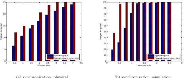
Spread-space. A visit statement employing spread-space is enclosed within a normal Java while loop. The en-closing loop repeatedly attempts to initiate the visit; these attempts will fail until sufficient camera nodes are available to achieve the desired spatial distribution. This approach visits more cameras than are actually needed; photos are timestamped upon capture, and a post-processing step se-lects the photos that were taken closest together in time.

Spread-space, Sync-time. Sarana’s sync-time feature in conjunction with spread-space. sync-time ensures that once the scheduler decides to issue tasks to remote nodes, those tasks will be scheduled to run at approximately the same time. spread-space ensures that the scheduler will not choose to issue tasks until the desired spatial distribu-tion is possible. The current implementadistribu-tion of sync-time is not sophisticated and relies on GPS synchronization of device clocks, which has a precision of approximately one second. We use it to demonstrate that even with a primi-tive implementation, this language feature is useful.

The physical trials in this section use a configuration con-taining 25 randomly placed camera nodes; an image is ob-tained from every camera. The camera service is not active on every node at the start of a trial; rather, it is activated

(10)

0 0.5 1 1.5 2 2.5 3 3.5 4 4.5 0 5 10 15 20 25 Window Size Images Acquired Spread−space Spread−space, sync−time

(a) synchronization, physical

0 0.5 1 1.5 2 2.5 3 0 10 20 30 40 50 60 70 80 90 100 Window Size Images Acquired Spread−space Spread−space, sync−time (b) synchronization, simulation

Figure 8: Crowd Estimation with temporal synchronization, baseline algorithm (spread-space only) and sync-time. Graphs show the maximum number of photographs timestamped in any time window of the given size.

at a randomly chosen later time (representing the choice of each crowd member to turn on their cellphone and/or par-ticipate in the measurement). For any given time window size w, we compute the maximum number of photos that are timestamped within w seconds of each other. The experi-ment was repeated 10 times and the results of these trials were averaged.

The results are given in Figure 8(a), and show that the Sarana scheduling scheme can achieve more accurate syn-chronization of tasks than an application could achieve on its own. When high accuracy is required (smallest time win-dow), the improvement is up to 86%.

The simulated trials in this section use a configuration containing 300 randomly placed camera nodes, of which we sample 100 in a spatially distributed fashion. The results are consistent with our physical trials (Figure 8(b)).

5. RELATED WORK

The system described in this paper builds on two prior efforts by our research group. The imperative, macropro-gramming model based on parallel loops is drawn from Spa-tialViews [20]. The notion of node selection to satisfy a bud-get was developed in a prior version of Sarana [7]. Neither of these systems exploited the spatiotemporal properties of an application, and neither included a notion of dynamic program feedback, the key ideas in our current work.

Programming abstractions. There is substantial prior work in the area of programming models and abstractions for wireless sensor networks. Many systems focus on providing a single-node programming abstraction, together with fea-tures that allow communication between the nodes. Such systems include TinyOS [8], nesC [4], abstract regions [27], Eon [24], and Pixie [14]. Other systems provide program-ming abstraction that include the overall interactions be-tween individual nodes, i.e., provide a whole network pro-gramming model. In the sensor network community, such a programming approach is referred to as

macroprogram-ming. Kairos [1], Regiment [18], WaveScripts [17], Kairos

[6], Pleiades [13], SpatialViews [20] and Spatial Program-ming [2] all support macroprogramProgram-ming.

Systems to program dynamic and sensor network vary sig-nificantly in the language paradigm and computation repre-sentation that they have chosen. Systems may use an imper-ative loop model [6, 26, 13, 20, 2], a functional model with data streams [18, 17], or data-flow based models [1, 24].

Target systems. Our primary targets are opportunis-tic, heterogeneous dynamic networks of mobile (e.g., smart phones [9, 22, 10]) and stationary devices (e.g., surveillance cameras, weather stations). These are distinct from sensor networks in that the application programmer does not con-trol all devices in the network, the services they provide, or their resource usage policies. It is the responsibility of the owner of each device to establish resource management policies suitable for that particular device.

Adaptations to resource/cost changes. There is a substantial body of work addressing the adaptation of soft-ware requirements to changing resource availabilities. The Odyssey project was one of the first to address this issue [21]. One of the main challenges is to decide what level of abstraction should be exposed to the programmer, and what controls should be provided to react to changing re-source availabilities. ECOSystem uses the operating system to assign energy budgets to processes, and perform energy accounting [28]. Eon [24], Wishbone [19], and Pixie [14] perform resource management on a single node, whereas Peloton [26], SORA [16] and Mainland et al. [15] have a network-centric view where resources are managed across a set of nodes in order to preserve or optimize network utility. In contrast, Sarana manages resources and allocates tasks across a potentially large set of nodes in order to improve the utility of the application execution.

To the best of our knowledge, Sarana is the first system that allows a user to specify spatiotemporal heuristics at the language level that are harnessed at run time to adaptively schedule the execution of an application on a set of mobile nodes.

(11)

6. CONCLUSION AND FUTURE WORK

We showed that the performance of resource-constrained dynamic network applications can be significantly improved by exploiting their spatiotemporal properties. This improve-ment can take the form of better outcomes for the same re-source budget, or comparable outcomes at much lower cost. We are currently investigating possible spatiotemporal op-timizations and their impact on program performance. Par-ticularly, we are looking at traditional compile-time loop level optimizations such as loop interchange, loop distribu-tion, and loop fusion in this new context.

Privacy and security are clearly important issues in any mobile network environment where resources might be shared. Resource-constrained systems will require tradeoffs between the degree of security and the resources required to maintain that degree of security. We are currently exploring strategies such as sandboxing (e.g., [5]) and trusted computing (e.g., [23]). We believe that our framework can be extended to allow the programmer to express security preferences effec-tively.

7. ACKNOWLEDGEMENTS

This work has been partially supported by NSF awards CNS-EHS #0615175 and #0614949.

8. REFERENCES

[1] A. Awan, S. Jagannathan, and A. Grama.

Macroprogramming heterogeneous sensor networks using COSMOS. In EuroSys’07, Lisbon, Portugal, March 2007. [2] C. Borcea, C. Intanagonwiwat, P. Kang, U. Kremer, and

L. Iftode. Spatial programming using Smart Messages: Design and implementation. In International Conference

on Distributed Computing Systems (ICDCS’04), Tokyo,

Japan, March 2004.

[3] J. Burke, D. Estrin, M. Hansen, A. Parker, N. Ramanathan, S. Reddy, and M.B. Srivastava. Participatory sensing. In World Sensor Web Workshop,

ACM SenSys’06, Boulder, Colorado, October 2006.

[4] D. Gay, P. Levis, R. von Behren, M. Welsh, E. Brewer, and D. Culler. The nesC language: A holistic approach to networked embedded systems. In ACM SIGPLAN

Conference on Programming Language Design and Implementation (PLDI’03), 2003.

[5] I. Goldberg, D. Wagner, R. Thomas, and E.A. Brewer. A secure environment for untrusted helper applications confining the wily hacker. In SSYM’96: Proceedings of the

6th conference on USENIX Security Symposium, Focusing on Applications of Cryptography, 1996.

[6] R. Gummadi, O. Gnawali, and R. Govindan.

Macro-programming wireless sensor networks using Kairos. In International Conference on Distributed Computing in

Sensor Systems (DCOSS), June 2005.

[7] P. Hari, K. Ko, E. Koukoumidis, U. Kremer, M. Martonosi, D. Ottoni, L. Peh, and P. Zhang. Sarana: Language, compiler and run-time system support for spatially aware and resource-aware mobile computing. Philosophical

Transactions of the Royal Society A, 366(1881), July 2008.

[8] J. Hill, R. Szewczyk, A. Woo, S. Hollar, D. Culler, and K. Pister. System architecture directions for network sensors. In Architectural Support for Programming

Languages and Operating Systems (ASPLOS’00), 2000.

[9] Apple Inc. iphone - an internet connected multimedia smartphone. http://www.apple.com/iphone.

[10] Google Inc. Android - an open handset allicance project. http://code.google.com/android.

[11] javaparser. http://code.google.com/p/javaparser.

[12] C. Koelbel, D. Loveman, R. Schreiber, G. Steele, and M. Zosel. The High Performance Fortran Handbook. MIT Press, 1994.

[13] N. Kothari, R. Gummandi, T. Millstein, and R. Govindan. Reliable and efficient programming abstractions for wireless sensor networks. In ACM SIGPLAN Conference on

Programming Language Design and Implementation (PLDI’07), June 2007.

[14] K. Lorincz, B. Chen, J. Waterman, G. Werner-Allen, and M. Welsh. Resource aware programming in the Pixie OS. In

ACM Conference on Embedded Networked Sensor Systems (SenSys’08), Raleigh, NC, November 2008.

[15] G. Mainland, L. Kang, S. Lahaie, D.C. Parkes, and M. Welsh. Using virtual markets to program global behavior in sensor networks. In Proc. 11th ACM SIGOPS

European Workshop, Leuven, Belgium, 2004.

[16] G. Mainland, D. Parkes, and M. Welsh. Decentralized, adaptive resource allocation for sensor networks. In

USENIX/ACM Symposium on Networked System Design and Implementation (NSDI’05), Boston, MA, May 2005.

[17] R. Newton, L Girod, M. Craig, S. Madden, and G. Morrisett. Design and evaluation of a compiler for embedded stream programs. In ACM SIGPLAN-SIGBED

Conference on Languages, Compilers, and Tools for Embedded Systems, Tucson, AZ, June 2008.

[18] R. Newton, G. Morrisett, and M. Welsh. The Regiment macroprogramming system. In Information Processing in

Sensor Networks (IPSN’07), Cambridge, MA, April 2007.

[19] R. Newton, S. Toledo, L. Girod, H. Balakrishnan, and S. Madden. Wishbone: Profile-based partitioning for sensornet applications. In USENIX/ACM Symposium on

Networked System Design and Implementation (NSDI’09),

Boston, MA, April 2009.

[20] Y. Ni, U. Kremer, A. Stere, and L. Iftode. Programming ad-hoc networks of mobile and resource-constrained devices. In ACM SIGPLAN Conference on Programming

Language Design and Implementation (PLDI’05), Chicago,

IL, June 2005.

[21] B. Noble, M. Satyanarayanan, D. Narayanan, J.E. Tilton, J Flinn, and K. Walker. Agile application-aware adaption for mobility. In ACM Symposium on Operating System

Principles (SOSP’97), Saint-Malo, France, October 1997.

[22] OpenMoko. Linux based open source mobile phones. [23] R. Sailer, X. Zhang, T. Jaeger, and L. van Doorn. Design

and implementation of a tcg-based integrity measurement architecture. In SSYM’04: Proceedings of the 13th

conference on USENIX Security Symposium, 2004.

[24] J. Sorber, A. Kostadinov, M. Garber, M. Brennan, M.D. Corner, and E.D. Berger. Eon: A language and runtime system for perpetual systems. In ACM Conference on

Embedded Networked Sensor Systems (SenSys’07), Sydney,

Australia, November 2007.

[25] S. Velipasalar, J. Schelessman, C-Y. Chen, W. Wolf, and J.P. Singh. SCCS: a scalable clustered camera system for multiple object tracking communicating via message passing interface. In Proceedings of International

Conference on Multimedia and Expo, 2006.

[26] J. Waterman, G.W. Challen, and M. Welsh. Peloton: Coordinated resource management for sensor networks. In

12th Workshop on Hot Topics in Operating Systems (HotOS-XII), May 2009.

[27] M. Welsh and G. Mainland. Programming sensor networks using abstract regions. In USENIX/ACM Symposium on

Networked System Design and Implementation (NSDI’04),

March 2004.

[28] H. Zeng, C.S. Ellis, A.R. Lebeck, and A. Vahdat. Ecosystem: Managing energy as a first class operating system resource. In Tenth International Conference on

Architectural Support for Programming Languages and Operating Systems (ASPLOS-X), San Jose, CA, October