Aerodynamic benefits of boundary layer ingestion for the D8 double-bubble aircraft

(1)

Aerodynamic Benefits of Boundary Layer Ingestion for the

D8 Double-Bubble Aircraft

by

Cecile

J. Casses

B. Eng., Ecole Centrale Paris, 2013

Submitted to the Department of Aeronautics and Astronautics in partial fulfillment of the requirements for the degree of

Master of Science in Aeronautics and Astronautics at the

MASSACHUSETTS INSTITUTE OF TECHNOLOGY

September 2015

@

ARCHIES

MASSACHUSETTS INSTITUTE OF TECHNOLOGY

OCT 14 2015

LIBRARIES

A uthor ... C ertified by ...

Signature redacted

Department of Aeronautics and Astronautics August 19, 2015

Signature redacted

. . Edward M. Greitzer H. N. Slater Professor of Aeronautics and Astronautics

Certified by...

Thesis Supervisor

Alejandra Uranga Research Engineer, Department of Aeronautics and Astronautics Thesis Supervisor

Signature redacted

Accepted by... ... Paulo C. Lozano

Associate Professor of Aeronautics and Astronautics Chair, Graduate Program Committee

Signature redacted

(2)

(3)

Aerodynamic Benefits of Boundary Layer Ingestion for the

D8 Double-Bubble Aircraft

by

Cecile Casses

Submitted to the Department of Aeronautics and Astronautics on August 19, 2015, in partial fulfillment of the

requirements for the degree of

Master of Science in Aeronautics and Astronautics

Abstract

This thesis describes experimental assessments of the aerodynamic boundary layer ingestion (BLI) benefit of the D8 advanced civil aircraft design. Two independent methods were applied for 1:11 scale (4.1 m wingspan) powered aircraft model experi-ments in the NASA Langley 14x22-foot Subsonic Wind Tunnel. The metric used as a surrogate for fuel consumption was the input mechanical flow power, and the benefit was quantified by back-to-back comparison of non-BLI (podded) and BLI (integrated)

configurations.

The first method (indirect) was the estimate of mechanical flow power based on the measured electrical power to the propulsors, plus supporting experiments to char-acterize the efficiencies of the fans and the electric motors that drive them, at the MIT Gas Turbine Laboratory. The second method (direct) was the direct integra-tion of flowfield measurements, from five-hole probe surveys at the inlet and exit of the propulsors, which provided flow angles, velocity components, and pressure coeffi-cients. Data were taken at different wind tunnel speeds, and conditions to determine overall performance dependence on non-dimensional power and angle of attack. At the simulated cruise point, the first method gave a measured aerodynamic BLI ben-efit of 7.9% 1.5% at 70 mph tunnel velocity, and 8.5% 1.5% at 84 mph, and the second method gave a measured benefit of 8.1%t3.3% at 70 mph, and 12.2% 3.4% at 84 mph. For the aircraft models examined, the aerodynamic benefit was found to come primarily from a decrease in the propulsor jet velocity (increase in propulsive efficiency) and thus a decreased jet dissipation, with the contribution from decreased wake and airframe dissipation being roughly an order of magnitude smaller.

Thesis Supervisor: Edward M. Greitzer

Title: H. N. Slater Professor of Aeronautics and Astronautics

Thesis Supervisor: Alejandra Uranga

(4)

(5)

Acknowledgments

This research was supported by NASA's Fundamental Aeronautics program, the

NASA Fixed Wing Project under Cooperative Agreement NNX11AB35A.

I would like to start by thanking my advisor, Edward Greitzer, who enabled me

to have the MIT Energy Initiative Fellowship as a financial support during my first year at MIT. His infinite technical support and advice in the past two years helped me learn how to solve engineering problems in a rigorous manner. I want to recognize Neil Titchener for his guidance through this project, the ski trip, and the British spirit, Alejandra Uranga for her support and meticulous help with the thesis writing. Last but not least, Professor Drela for sharing his deep knowledge during his amazing courses. I appreciate the assistance of Robin Courchesne-Sato who made everything possible at the Gas Turbine Lab.

I acknowledge the help of all the members of the N+3 team for making all of that come true. A special thanks goes to Michael, and Nina who were always present to explain with patience everything they worked on on the project and to help me move forward. Not to forget Elise, Arthur Huang, David Hall, and Adam Grasch for their irreplaceable contributions. Thank you to those who helped during the Langley tests, to James Jensen and Shishir Pandya at NASA Ames for the CFD, and to Gregory Gatlin at NASA Langley Research Center.

And if you think MIT is not hard enough, it is forgetting Devon that comes to your office and asks you aerodynamics questions that you have no clue about. But, of course, he knows the answer! Thanks for keeping my mind busy, for your optimism, for your patience when I made you repeat the same sentence five times, and for your friendship. The daily tea time with Devon, Elise, Lucie, and Sebastien is above all the main reason for the completion of this thesis and created an atmosphere more joyful, optimistic, and social at the GTL.

These years would have never been the same without my friends, those who stayed in France and those I met in Boston, and the ORCers. Particularly, my roommates Ludo, Virgile, and Mapi with whom I shared meals, joys, sadness, and

(6)

more! Thanks to Claire-Marine and Pierre for all our life talks. To the Trapuchette and the 109 Otis for all the social events. Most importantly, I am sincerely grateful to Maximilien for his support through the last month of my master and for my career decision, and his love.

Lastly, all of that would have never been possible without the support, the love, and the trust in me of my family. I will never forget all the efforts that my parents, my brothers, my grandma, and my godfather put into this adventure. Not to mention, FREE, the French carrier, that enabled my little brother to call me from France everyday!

(7)

List of Figures

1-1 Cross-section, side, top, and back views of the D8 aircraft from

[5].

25

1-2 Difference of force definitions between non-BLI propulsors (left) and BLI propulsors (right) . . . . 26 1-3 Power and dissipation sources for the non-BLI and BLI configurations.

C redit: H all. . . . . 27

1-4 Model configurations of the D8 aircraft tested at NASA Langley. Credit: L ieu . . . . 29 1-5 Dimensions of the D8 propulsor for a) the non-BLI configuration and

b) the BLI configuration. Units in inches . . . . 30 1-6 Differences between plug 1 (small), 3 (medium), and 5 (big) . . . . . 31 1-7 D8 in the NASA Langley Wind Tunnel. in September 2014. Credit:

NASA/George Homich. . . . . 32

2-1 (a) Top and front view, and (b) 3D view of the dynamometer rig to m easure torque . . . ... . . .. . . . . 37

2-2 Calibration curves: a) Calibration factor, k, against force in Newtons;

b) Applied force in Newtons against measured load cell voltage . . . . 39 2-3 a) Electrical power and b) torque versus motor speed for the three

propellers . . . . 41 2-4 Superimposition of propeller operating points from calibration

mea-surements and propulsor operating points from Langley at 70 mph a) for BLI configuration and b) for non-BLI configuration . . . . 42

(12)

2-5 Contour of motor efficiency, rim, for motor 6. Langley test operating points are indicated by symbols, green for BLI and black for non-BLI

configuration. . . . . 44

2-6 Polynomial fit of the mean efficiency with uncertainty error bars (elec-tronic box 1, power supply 1, motor 6) . . . . 48

2-7 RPM measurements from the photogate and the back-EMF signal with

their tim e averages . . . . 50 2-8 Relative contributions of the different sources in percentage on the

different uncertainties: a) Calibration factor; b) Torque; c) Efficiency 52 3-1 Setup for the propulsor characterization experiments. Credit: Siu. . . 56

3-2 Straight five-hole probe . . . . 57

3-3 Control volume for mechanical flow power integration . . . . 58

3-4 Motor efficiency against flow coefficient for both propulsors, different

wheel speeds, and distorted or non-distorted flow . . . . 61 3-5 (a) Stagnation pressure rise coefficient and (b) overall efficiency against

flow coefficient for both propulsors, different wheel speeds, and

dis-torted or non-disdis-torted flow . . . . 62 3-6 Fan efficiency against flow coefficient for both propulsors, different

wheel speeds, and a) non-distorted and b) distorted flow . . . . 63 3-7 Fan efficiency against flow coefficient for both propulsors, with

dis-torted and non-disdis-torted flow at a) 10600 RPM (Langley cruise at 70

mph), and b) 13500 RPM (Langley cruise at 84 mph) . . . . 64

3-8 Net streamwise force coefficient against a) electrical power coefficient and b) shaft power coefficient at 70 mph, plug 3, and 2' angle of attack for the BLI configuration. The dashed line at Cx = 0 indicates the simulated cruise condition. . . . . 67

(13)

3-9 Curvefits of net streamwise force coefficient against a) electrical power

coefficient and b) shaft power coefficient at 70 mph, plug 3, and 2' angle of attack for the BLI configuration. The dashed line at Cx = 0 indicates the simulated cruise condition. . . . . 68 3-10 Curvefits of net streamwise force coefficient against a) electrical power

coefficient and b) shaft power coefficient at 84 mph, plug 3, and 2' angle of attack for the BLI configuration. The dashed line at Cx = 0 indicates the simulated cruise condition. . . . . 69 3-11 Net streamwise force coefficient against flow power coefficient at a) 70

mph and b) 84 mph, plug 3, and 2' angle of attack for both the non-BLI and the non-BLI configurations. The dashed line at Cx = 0 indicates the simulated cruise condition. . . . . 70 3-12 Non-dimensionalized mechanical flow power as a function of propulsive

efficiency at 84 mph for BLI and non-BLI configurations, numbers refer to different area nozzle plugs . . . . 75 3-13 Non-dimensionalized shaft power as a function of propulsive efficiency

at 84 mph for BLI and non-BLI configurations, numbers refer to dif-ferent area nozzle plugs . . . . 75

3-14 Fan efficiency against flow coefficient at 84 mph for both configurations and for a) the left propulsor and b) the right propulsor . . . . 76 3-15 Uncertainty propagation for the mechanical flow power coefficient with

the indirect measurement method . . . . 78

4-1 Survey grids for a) the non-BLI exit configuration, b) the BLI exit configuration with plug 3, and c) the BLI inlet configuration . . . . . 83

4-2 Survey planes for a) the non-BLI exit configuration, and b) the BLI inlet and exit configurations. Flow goes to the right. Credit: Jensen and Pandya, NASA Ames. . . . . 84 4-3 Comparison of the actual and desired coordinates for the survey grid 86

(14)

4-5 Angles and velocity convention. Credit: Siu [1]. . . . .8

4-6 Contours of stagnation pressure coefficient, C,, for (a) the inlet and

(b) the exit of the propulsor on the BLI configuration with plug 3 at

cruise condition at 70 mph . . . . 89

4-7 Contours of (a)-(b) pitch angle, (c)-(d) yaw angle, and (e)-(f) ratio of streamwise velocity to freestream velocity for the inlet (left plots) and exit (right plots) of the propulsors on the BLI configuration with plug

3 at cruise condition at 70 mph . . . . 90

4-8 Contours of (a) stagnation pressure coefficient, (b) pitch angle, (c) yaw angle, and (d) ratio of streamwise velocity to freestream velocity at the propulsor exit for the non-BLI configuration with plug 3 at cruise condition at 70 m ph . . . . 91

4-9 Contours of stagnation pressure coefficient for BLI inlet (left figures) and BLI exit (right figures) with (a)-(b) plug 1, (c)-(d) plug 3, and (e)-(f) plug 5 at cruise condition at 84 mph . . . . 93

4-10 Contours of pitch angle for BLI inlet (left figures) and BLI exit (right figures) with (a)-(b) plug 1, (c)-(d) plug 3, and (e)-(f) plug 5 at cruise condition at 84 mph . . . . 94

4-11 Contours of yaw angle coefficient for BLI inlet (left figures) and BLI exit (right figures) with (a)-(b) plug 1, (c)-(d) plug 3, and (e)-(f) plug

5 at cruise condition at 84 mph . . . . 95

4-12 Contours of ratio of streamwise velocity to freestream velocity for BLI inlet (left figures) and BLI exit (right figures) with (a)-(b) plug 1,

(c)-(d) plug 3, and (e)-(f) plug 5 at cruise condition at 84 mph . . . . 96

4-13 Contours of (a) stagnation pressure coefficient, (b) pitch angle, (c) yaw angle, and (d) ratio of streamwise velocity to freestream velocity for the propulsor exit for the non-BLI configuration with plug 3 at cruise condition at 84 m ph . . . . 97

(15)

4-14 Contous of stagnation pressure coefficient at the propulsor inlet for the BLI configuration at (a) start-of-climb, (b) top-of-climb, and (c)

descent with plug 3 . . . . 99 5-1 (a) Side view, and (b) top view of streamlines across the right propulsor

from numerical simulations, at 70 mph, BLI configuration, plug 1, 2' angle of attack, Cx = 0. Credit: Jensen and Pandya, NASA Ames. . 103 5-2 (a) Edge of streamtube through the right propulsor, and (b) survey

(red crosses) and integration (black circles) grids of the right propulsor at 70 mph for the BLI inlet . . . . 103 5-3 Side view of streamlines across the left propulsor from numerical

sim-ulations, at 70 mph, non-BLI configuration, plug 1, 2' angle of attack, Cx = 0. Credit: Jensen and Pandya, NASA Ames. . . . . 105

5-4 Edge of exit streamtube, and exit survey (red crosses) and integration (black circles) grids for the right propulsor at 70 mph for (a)-(c) the BLI, and (b)-(d) the non-BLI configurations . . . . 105 5-5 Mechanical flow power coefficient and non-dimensionalized mass flow

versus number of points of the integration grid for the right (a)-(b) BLI inlet, (c)-(d) BLI exit, and (e)-(f) non-BLI exit at 70 mph . . . . 107 5-6 (a) Mechanical flow power coefficient, and (b) non-dimensionalized

mass flow integrated in the survey plane at 70 mph and 84 mph for the BLI inlet, BLI exit, and non-BLI exit. 'L' means left side, and 'R' m eans right side. . . . . 110 A-i Setup for the propulsor characterization experiments. Credit: Siu. . . 118 A-2 Non-dimensionalized volumetric flow rate against non-dimensionalized

inferred velocity for inlet surveys for the three inlet measurements, no distortion . . . . 121

A-3 Non-dimensionalized volumetric flow rate from FHP against non

(16)

A-4 Non-dimensionalized volumetric flow rate against non-dimensionalized inferred velocity for a) inlet surveys and b) exit surveys with distortion 123

A-5 Exit survey grid in black dots. Black lines represent the separation of

the survey in the circumferential direction. Magenta circles represent the plug 1 geometry and the propulsor nacelle. Blue lines represent the geometry of the bifurcation. . . . . 124

B-1 Ratio of density between exit and inlet of the propulsor with and with-out distortion introduced for the MIT experiments . . . . 126

(17)

List of Tables

1.1 NASA goals for N+3 generation of aircraft . . . . 23

1.2 Propulsor design yaw and pitch angles in the airframe reference frame. C redit: Lieu. . . . . 28

1.3 Plug characteristics where fan area, Af, is 0.0159 m2 . . . . 31

2.1 Motor efficiencies at simulated cruise condition for motors 6 and 7 using electronic box 1, and power supply 1 . . . . 43 2.2 Summary of motor efficiencies at simulated cruise conditions:(p) for

non-BLI, (iL) for left BLI propulsor, and (iR) for right BLI propulsor 46

2.3 Efficiency values at simulated cruise conditions for electronic box 1 and motors 6 and 7 with repeatability uncertainty at 95% confidence interval 48 2.4 Independent variables uncertainty for motor efficiency . . . . 49

2.5 Fractional uncertainties in the efficiency . . . . 51 2.6 Comparison between uncertainties from the statistical method and the

propagation method on motor efficiency in % . . . . 52 3.1 Summary of electrical, shaft, and mechanical flow power coefficients

and flow coefficient, and propulsive efficiency for BLI and non-BLI configurations at simulated cruise condition, 70 mph . . . . 77 3.2 Summary of electrical, shaft, and mechanical flow power coefficients

and flow coefficient, and propulsive efficiency for BLI and non-BLI configurations at simulated cruise condition, 84 mph . . . . 77 3.3 Independent variable uncertainty for BLI benefit . . . . 79

(18)

3.4 Comparison between uncertainties from the statistical method and the

propagation method on BLI benefit at 70 and 84 mph in % . . . . 79

4.1 Number of points for the survey grids for all configurations with plug 3 82 5.1 Number of radial, circumferential, and total points for the different integration grids . . . . 108

5.2 Mechanical flow power for BLI inlet, BLI exit, and non-BLI exit with plug 3 at 70 and 84 mph. 'L' refers to the quantity for the left side, 'R' refers to the quantity for the right side, and 'Tot' refers to the total quantity including left and right sides. . . . .111

5.3 Uncertainty for the mechanical flow power coefficient for the indirect m ethod . . . . 112

6.1 Aerodynamic BLI benefit for the two experimental methods and CFD 114 A. 1 Summary of the volumetric flow rates associated with different instru-mentations and different assumptions . . . . 120

C. 1 Matrix of power sweep conditions from Entry 1 . . . . 128

C.2 Matrix of power sweep conditions from Entry 2 . . . . 129

(19)

Nomenclature

Latin Letters

Af fan area

CD drag coefficient

CPO stagnation pressure coefficient (= (po - po,)/qo)

CPE electric power coefficient (= PE/qoVoSref)

CPS shaft power coefficient (= Ps/q0VoSref)

CPK mechanical flow power coefficient (= PK1/qV.Sref)

Cop rotor tip chord

Cx net streamwise force coefficient (= Fx/qSref)

D drag force

Dfan D8 propulsor fan diameter

fBLI percentage of fuselage boundary layer ingested by the propulsors

FN force

Fx net streamwise force (= D - T)

i indexing variable or current

k motor calibration factor

kc calibration factor for the wind tunnel dynamic pressure

L length

mh mass flow

M Mach number

h unit normal vector

(20)

Nr number of radial points in flow surveys

No number of circumferential points in flow surveys Ntot number of total points in flow surveys

p static pressure

PO stagnation pressure

P power

PE electrical power

Ps shaft power

PK mechanical flow power

PK mechanical flow power integrated in the measurement plane

PSC BLI benefit (= (CPK,non-BLI - 0 PK,BLI)/PK,non-BLI) q dynamic pressure (= 0.5pV2)

qc kiel probe dynamic pressure in the MIT GTL wind tunnel

Q

torque or volumetric flow rate

r radial location

Re Reynolds number

S standard deviation

S surface integration variable

Sref D8 model reference area

t t-distribution correction factor

T thrust force

Utip fan tip speed

v voltage

V velocity vector

V speed

V , V, V1 Cartesian velocity components

Vo reference velocity for the MIT GTL experiments

VLC load cell voltage value

W weight

Y, Z cartesian coordinates of survey points;

(21)

Greek Letters

a D8 model angle of attack or pitch flow angle for flow surveys

#

D8 model side slip angle or yaw flow angle for flow surveys

r7 efficiency

I7 heat capacity ratio

1 air viscosity

Q motor wheel speed

wr stagnation pressure ratio

flow coefficient dissipation quantity

stagnation pressure rise coefficient

p air density

T stagnation temperature ratio

- measurement uncertainty

Superscripts

( )'

non-BLI configuration quantity

Subscripts

(

)BLI BLI configuration (or integrated)

( )

fan quantity

(

) propulsor inlet quantity

(

)jet propulsor jet quantity

(

)Lc load cell quantity

(

) left left propulsor quantity

(

)m electric motor quantity

(

)non-BLI non-BLI configuration (or podded)

( )0 overall quantity

(22)

(

)ref reference quantity

( )0 quantity at station 0 in the MIT GTL wind tunnel

( )right right propulsor quantity

( )surf fuselage surface quantity

( )vortex vortex quantity

( )wake fuselage wake quantity

( )w weight quantity

( )o freestream (wind tunnel) quantity

Other Symbols

A () difference quantity

( ) mass-averaged quantity

Abbreviations

APC advanced precision composites

BLI boundary layer ingestion

CFD computational fluid dynamics

CV control volume

EMF electromotive force

ESC electronic speed controller

FHP five-hole probe

GTL Gas Turbine Laboratory

LTO landing, take off

MIT Massachusetts Institute of Technology

NASA National Aeronautics and Space Administration

NOx nitrogen oxyde

N+3 2025-2035 time frame

PS Pitot-static

(23)

Chapter 1 Introduction

In 2008, NASA put forward a solicitation for the development of advanced concepts and enabling technologies to address environmental challenges and performance im-provements for commercial transport aircraft entering in service in the 2025-2035 timeframe. Since then, in two separate phases, a team of MIT, Aurora Flight Sci-ences, and Pratt and Whitney, has been carrying out research to create and assess the conceptual design of the D8 aircraft that meets the NASA requirements of fuel burn reduction, noise reduction, and landing and take-off (LTO) nitrogen oxide (NOx) emissions. Although the goals have changed since 2008, as shown in Table 1.11, they are still aggressive enough that meeting them calls for a clean-sheet design.

A product of Phase I (September 2008 to March 2010) was the conceptual design

of the D8 subsonic transport to meet the NASA targets [2]. A key technology for aircraft fuel burn reduction was found to be Boundary Layer Ingestion (BLI). It is critical to assess BLI benefit because the technology has not been implemented on civil aircraft.

Table 1.1: NASA goals for N+3 generation of aircraft

Fuel burn Noise LTO NOx emissions

Goals (2008 [2]) -70% -71 EPNdB below stage 4 -80% below CAEP6

Goals (2013 [3]) -60% -52 EPNdB below stage 4 -80% below CAEP6

1_{EPNdB measures the effective perceived noise in decibels, and CAEP refers to the Committee}

(24)

A major focus of Phase II, from November 2010 to May 2015, therefore was

assessment of the BLI benefit for the D8. For this purpose, experiments in the NASA Langley 14x22-foot Subsonic Wind Tunnel [4], using a 1:11 scale powered D8 aircraft model, were designed and carried out. Numerical simulations of the model in the wind tunnel have also been conducted. This thesis describes the wind tunnel experiments and conceptual simulations to evaluate the BLI benefit.

1.1 The D8 Aircraft Concept

A three-view of the D8 aircraft concept as designed by Drela [2] is shown in Figure 1-1.

Often referred to as the 'double-bubble' in reference to the fuselage cross-section, the aircraft is designed to operate on the same missions as a B737-800 or an A320 (180 passengers, 3000 NM range transport). This twin-engine is predicted to require 66% less fuel burn than the 737-800 baseline if constructed with 2025-2035 level technology, or 33% if constructed with currently available technology

[5].

The aircraft design was found by simultaneous optimizations of the airframe, the engines, and the operations for a given mission, to achieve minimum fuel burn2_.

The main features of the aircraft are: two propulsors flush-mounted on the top aft fuselage under a pi-tail permitting 40% of the fuselage boundary layer to be ingested

by the propulsors; higher lift generated by the fuselage (18% vs 13% for a B737-800 [6]) allowing the wings to shrink; lift generated by the nose to decrease the size

of the horizontal tail; aircraft cruise Mach number of 0.72 to lower the wing sweep; pi-tail to lighten the horizontal tail compared to T-tail and to provide noise shielding for the propulsors; and double-bubble shape for two aisles to reduce passenger loading

and unloading times.

2

The multi-disciplinary tool used was TASOPT 2.0, TASOPT stands for Transport Aircraft System OPTimization [2].

(25)

- -

--~EJ

a

0 0

v 0

Figure 1-1: Cross-section, side, top, and back views of the D8 aircraft from

[5].

"I

(26)

-1.2

Boundary Layer Ingestion

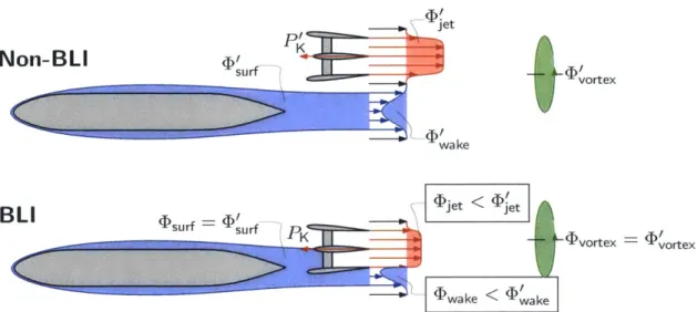
Boundary Layer Ingestion (BLI) occurs when the propulsors ingest some part of the flow that is decelerated due to the friction with a surface. For the D8, the propulsors ingest roughly 40% of the fuselage boundary layer. Previous studies have estimated that BLI can reduce power requirement between 5 and 10% [7, 8] depending on how much boundary layer is ingested and the boundary layer shape parameters. With BLI, the exhaust jet and the fuselage wake are co-located so there is a reduced kinetic energy defect in the wake, and an increase in propulsive efficiency for the jet, and thus a reduced power consumption. It is difficult, however, to separate the forces due to the propulsor and those due to the airframe, as implied by Figure 1-2. The left-hand side shows a conventional (non-BLI) propulsion system and the right-hand side illustrates that the jet is embedded in the wake so thrust and drag generating flows are intermingled.

To provide a more appropriate framework for analyzing integrated systems, Drela introduced a power balance method

[9]

rather than working in terms of forces. The mechanical flow power transmitted by the propulsors to the flow results in several different dissipation sources: jet, wake, surface, boundary layers, and trailing vortex. These sources are sketched in Figure 1-3 in which the quantities associated with the non-BLI configuration are primed, and those for the BLI case are unprimed. The jet and wake dissipations are lower for the BLI configuration, while the surface dissipation and vortex dissipations are nearly equal (the estimated difference is less than 1%) for BLI and non-BLI configurations.

A mechanical flow power coefficient, CPK, can be defined by the ratio of

me-Figure 1-2: Difference of force definitions between non-BLI propulsors (left) and BLI propulsors (right)

(27)

Pf

Non-BLI

7urJ- _vortex

wake

BLI

(Diet < DJet

K vortex = Dvortex

Dwake < (wake

Figure 1-3: Power and dissipation sources for the non-BLI and BLI configurations. Credit: Hall.

chanical flow power, PK, to a reference power, 0.5pooV3Sre by

PK

1PK

0. 5pooV30Sref

The subscript oc represents freestream quantities and the reference area, Sref, cor-responds to the area of the exposed wings plus the virtual wing extending through

the fuselage. The density of the freestream flow is po, and VOo is the incoming flow velocity. The aerodynamic BLI benefit' is quantified by comparison of non-BLI and BLI configurations, and defined as a power saving coefficient, PSC, as

BLI Benef it = CPK,non-BLI - K,BLI)

CPK,non-BLI

This definition is consistent with Smith's power saving coefficient, PSC [7].

Assessing the BLI benefit is possible using data obtained from wind tunnel

experiments with a powered scale model, as is described in this thesis and previous

MIT N+3 publications ([10], [5], [1], [11], [12]).

3

There are others systems benefits for the BLI configuration, which are described in [6]. This thesis examines the aerodynamic benefit only.

(28)

1.3 NASA Langley Experiments

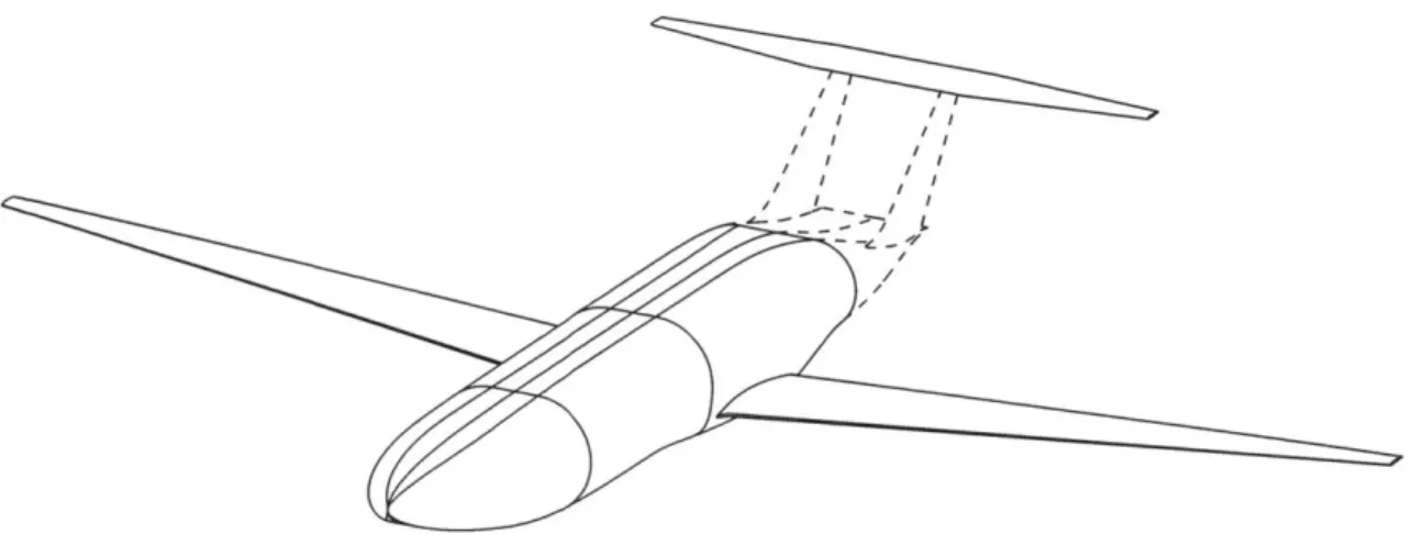
Three configurations of the D8 were tested at 1:11 scale as depicted in Figure 1-4. Fig-ure 1-4(a) shows the unpowered configuration with which the flow on the fuselage can be assessed. The horizontal tail and the front fuselage, which are drawn in black lines, are common to the three configurations to facilitate back-to-back comparison. The tail, which can be changed, is drawn with dashed lines. There are also two powered

configurations with propulsors that have electric fans. The non-BLI configuration (also referred to as 'podded') is shown in Figure 1-4(b) and the BLI configuration (referred to as 'integrated') is shown in Figure 1-4(c).

Each propulsor consists of a nacelle, an Aero-naut TF8000 fan stage (rotor and stator), an electric motor driving the fan, and a nozzle plug. Figure 1-5(a) is a drawing of the BLI propulsor and Figure 1-5(b) a drawing of the non-BLI propulsor. The propulsors were designed to be inserted in either the BLI or non-BLI configurations, again to allow back-to-back comparisons in evaluation of BLI benefit. Table 1.2 summarizes the angles at which the propulsors are titled and pitched.

Three nozzle plugs, shown in Figure 1-6, were manufactured to vary the mass flow through the propulsors. The plugs could be changed on the model without removing any other part. Table 1.3 summarizes the different plugs and the ratio of the nozzle areas to the fan frontal area.

A first-time back-to-back comparison of BLI and non-BLI configurations to

obtain an evaluation of BLI was carried out in a series of experiments in the NASA Langley 14x22-foot Subsonic Wind Tunnel. These experiments are referred to as the Langley tests.

There were two series of wind tunnel entries. The first entry, August and

Table 1.2: Propulsor design yaw and pitch angles in the airframe reference frame. Credit: Lieu.

Configuration Design yaw angle design pitch angle

BLI 30 1.50

(29)

(a) Unpowered configuration: common body in dark and interchangeable tail in dashed lines

0 10 50 in

(b) non-BLI configuration

0 10 50 in

(c) BLI configuration

Figure 1-4: Model configurations of the D8 aircraft tested at NASA Langley. Credit: Lieu.

(30)

3. 0 3.18 2.3 2.82 7.00 (b) BLI propulsor

Figure 1-5: Dimensions of the D8 propulsor for a) the non-BLI configuration and b) the BLI configuration. Units in inches

11.22 7.48

0.67

for pug changes

\1.77

(a) non-BLI propulsor

10.74 3. _{1 3.}₁ 0.48 2. 2 Point is fixes 2. 33 .1.70 3.22 2.82 I

(31)

Figure 1-6: Differences between plug 1 (small), 3 (medium), and 5 (big)

Table 1.3: Plug characteristics where fan area, Af, is 0.0159 m2 Plug Color in Figure 1 - 6 Ratio of nozzle area to fan area

1 black 0.535

3 blue 0.604

5 red 0.679

September 2013, included power sweeps where wind tunnel speed, angle of attack, and sideslip angle were fixed and motor speed was varied to obtain data for different net streamwise force coefficients (Cx). The range of parameters was: 2 - 8' for

an-gle of attack, - 150 for sideslip angle, 42 - 70 mph for wind tunnel speed, and 0

-13500 RPM for wheel speed. Pressure rake surveys, i.e. pressure measurements with

a rake at the inlet and exit of the propulsors, were also done. Integration of those pres-sure meapres-surements provided an estimate of mechanical flow power and BLI benefit.

Evaluation of the BLI benefit from the rake surveys was carried out by Lieu [11].

A second tunnel entry took place in August and September 2014. The maximum

wind tunnel speed was increased from 70 mph to 84 mph to reduce the experimental uncertainty. The experimental repeatability was also measured, for the same reason. Power sweeps, five-hole probe (FHP) surveys, and rake surveys were performed. The FHP surveys provide information on the flow ingested by the propulsors, as will be seen, to allow evaluation of the mechanical flow power.

A main interest was the simulated cruise condition, as cruise is where most fuel is

burnt. This condition is characterized by zero net streamwise force (Cx = 0) or, for a

(32)

conventional configuration, when drag and thrust are balanced. Off-design conditions were also considered: start-of-climb, top-of-climb, descent, cross-wind, and propulsor-out. The model had turbulence trips so the flow on the wings and the fuselage of the aircraft was turbulent, as would be the full-scale aircraft flow. The ratio of jet to freestream velocities at the design point was the same as the ratio for the full-scale aircraft based on information from TASOPT. Figure 1-7 shows the BLI configuration in the wind tunnel section.

Figure 1-7: D8 in the NASA Langley Wind Tunnel. in September 2014. Credit: NASA/George Homich.

(33)

1.4 Thesis Goals, Contributions, and Outline

In this thesis, the experimental evaluation of the D8 BLI benefit via two methods which are compared with each other and with computations (CFD) is described. The

two methods are:

1. Indirect Measurements of BLI benefit:

The only power measurement directly accessible at Langley was electrical power to the propulsor motors, PE, which needed to be converted into mechanical flow power, PK, the metric of interest. To enable the conversion, experiments were conducted at the MIT GTL 1x1 foot wind tunnel to characterize the electric motor efficiency, qtm, defined as the ratio of shaft power, Ps, to electric power, PE, and to characterize the propulsor and fan efficiency, rqf, defined as the ratio of mechanical flow power, PK, to shaft power, Ps [1]. The mechanical flow power and the electrical power are related by

PK -- ?7f?7mPE - (1.3)

2. Direct Measurement of BLI benefit:

The mechanical flow power is by definition [9] the volume flux of stagnation pressure, i.e. for incompressible flow:

PK J P(o. - po)V - UdS. (1.4)

Stagnation and static pressure fields were obtained from FHP surveys of the inlet and exit of the propulsor. The mechanical flow power, and hence the aerodynamic BLI benefit, was found from integrating these measurements at each plane.

A complimentary effort, led by Pandya at NASA Ames Research Center, focused

on numerically simulating the wind tunnel experiments. Chimera Grid Tools was used for the mesh and Overflow 2.2 for the solver. The simulations were run at 70 mph

(34)

with plug 1 for different net streamwise forces. The CFD results provide a third method of assessing the BLI benefit.

The thesis is organized as follows. Chapter 2 describes the motor calibration experiments. The data obtained from those experiments are used in Chapter 3 to evaluate the BLI benefit via the indirect method. The FHP surveys are described in Chapter 4 including characterization of the inlet flow at different conditions. In-tegration of these pressure measurements and evaluation of the BLI benefit using the direct method are presented in Chapter 5. Chapter 6 discusses the comparison between BLI benefit measurements, and computational results, as well as the ad-vantages associated with each method. Chapter 7 summarizes the results and the findings, and presents suggestions for future work.

(35)

Chapter 2 Motor Calibration Experiments

Evaluation of the BLI benefit implies determination of the mechanical power added to the stream by the propulsors, PK, in the BLI and non-BLI configuration. The me-chanical flow power was evaluated in two different ways as mentioned in Section 1.4. The goal of the first supporting experiments is to find the motor efficiency for the data obtained during the Langley tests, most importantly at the simulated cruise conditions (zero net streamwise force on the aircraft, Cx = 0) but also at off-design

conditions (Cx

#

0). The supporting experiments for the indirect method are

de-scribed first.

2.1 Experimental Methodology

2.1.1 Setup

The fans were driven by LMT 3040-27 motors1. The motor efficiency, defined as the ratio of shaft power to electrical power, is

TrIM -n =- (2.1)

PE iv

in which shaft power, Ps, is the product of torque,

Q,

and motor wheel speed, Q, and electrical power, PE, is the product of current, i, and voltage, v, across the motor. To

(36)

evaluate the efficiency, the motor torque, the motor speed, and the electrical power are needed.

The motor speed and power are inputs to the experiments and are measured. Torque is measured using the motor calibration rig shown in Figure 2-1. The rig was constructed by Grasch [13] but has had several improvements. The motor was positioned using clamps on a fixed solid mount composed of half-tube aluminum fixed to an aluminum base plate to reduce vibrations. An aluminum arm, screwed to the tube on one end, presses against the load cell on other end. The arm length is 200 mm so the load at the free end does not exceed 10 Newtons. The load cell is fixed on a support mounted on the base plate, with height such that the arm is horizontal. A 10 Newton single axis OMEGA LCMKD load cell was used because this has an appropriately small range of force at reasonable cost. The power to the motor is supplied by silicon wires. Efforts were made to prevent wire motion or deformation during testing to not disturb the torque measurement, and a metal shield was installed in front of the wires. A propeller is attached to the motor shaft using a collet type propeller adaptor (Grasch [13]). The system collet-propeller was mounted so no torque is exerted [14]. Three different propellers are used to span the range of forces representative of the loads exerted during the Langley tests: 10x07,

10x08, and 10x09 APC2 _{propellers. The propellers are defined with two numbers; the}

first is the diameter of the propeller in inches and the second is the pitch in inches per revolution. The experimental setup allows measurements of the force exerted on the load cell by the arm attached to the motor casing when the motor runs. From the known moment arm, the reaction torque from the motor on the motor casing, as well as the torque provided to the shaft, can be obtained.

2.1.2 Data Acquisition

The motor speed is acquired with a back-EMF signal from the motor and controlled

by a future-I-40.100 electronic speed controller (ESC) from Schulze Elektronik. The

(37)

Load cell Moment arm

Motor

Pro eller

(a) Top and front view

(b) 3D view

Figure 2-1: (a) Top and front view, and (b) 3D view of the dynamometer rig to

measure torque

I

Metal shield 9 E z

M5

Kn

1IT-1 FTI

(38)

current and voltage are obtained from the power supply3.

An electronic box, powered by the power supply, contains the ESC and outputs voltage and motor speed signals. Estimation of the motor winding temperature is enabled through a thermocouple4 _{placed on the skin of the motor. Voltage, current,}

RPM, temperature, and load cell voltage signals are linked to a National Instruments

DAQ-9188 box and processed with Labview.

The data in this report were acquired with electronic box 1 (one of the two used during the Langley tests), power supply 1 and motor 6 unless otherwise specified. Motors 6 (left propulsor) and 7 (right propulsor) were used during Entry 1. To make sure there were no issues during Entry 2, two new motors were used: motors 16 (left propulsor) and 13 (right propulsor). Another set was used and is mentioned in Chapter 3: motors 9 (left propulsor) and 15 (right propulsor).

2.1.3 Data Collection

The load cell was calibrated by hanging different weights (200 g and 500 g) at dif-ferent positions along the arm (100 mm and 50 mm from the load cell). At each point the voltage measured by the load cell is time-averaged over one and one half minutes. Figure 2-2(a) shows the measured calibration factor, k, against force, FN: the subscript N stands for Newton. Red crosses correspond to the calibration factors obtained using the different weights at different locations and the blue line represents the mean of all the calibration factors. The dashed lines indicate variation of 1%. Figure 2-2(b) gives weight force against measured load cell voltage values, VLC where the subscript LC denotes load cell value. The slope of the blue line is the mean calibration factor computed from data of Figure 2-2(a).

There is hysteresis in the load cell in that imposing a low loading (5250 RPM) after imposing a high loading (14000 RPM) gives a load cell value that differs from

3

2kW DCS 50-40 M16 power supply from Sorensen provides DC current at constant voltage by converting 240V 3-phase into 53V for the electronic box.

4

(39)

0.5 1 1.5 2 FN (N) (a) k 0.05 0.1 0.15 0.2 0.25 VLC (mV) (b) FN 2.5 3 3.5 0.3 0.35 0.4

Figure 2-2: Calibration curves: a) Calibration factor, k, against force in Newtons; b) Applied force in Newtons against measured load cell voltage

7.45 7.35 ----~ ------ ----- -~-F -7.3 L 0 4 weight FN=kV LC 3 2.5 2 1.5 0.5 z C 4

I0

(40)

the previous one. The difference is 3% at 10600 RPM. Consequently, load cell mea-surements were only recorded under conditions with the load (e.g. motor speed)

5

increasing from zero

A drift also occurs when going back to zero after loading. Imposing a high

load (running at 14000 RPM) prior to running the experiments reduced the drift to less than 1% between the first zero of the run and the last one. The drift has been accounted for by assuming linear drift with time and subtracting it from the load cell values.

2.2 Motor Experiments Results

Figure 2-3 shows curves of torque and electrical power versus motor speed for the three propellers. Each propeller was run four times. The crosses represent the points for the four different runs, and the line is a cubic spline curve-fit through the average of these points at each motor speed. Blue dotted line, red dashed line and black solid line correspond to 10x07, 10x08, and 10x09 propellers, respectively. The power and torque increase cubically with speed for each propeller and increase with loading

(higher propeller number) for the same motor speed.

Figure 2-4 shows the operating points from the Langley tests at 70 mph su-perimposed on the spline data interpolation. The operating points correspond to different angles of attack, a, wheel speed (RPM), and nozzle exit areas for the BLI configuration in the upper Figure 2-4(a), and the non-BLI configuration in the lower Figure 2-4(b)

[5].

The crosses represent data for the left motor and the circles for the right motor. Cyan data represent off-design conditions, i.e. angle of attack between

40 and 8'. Magenta data represent both cruise and off-design power settings at 2'.

Almost all the points lie within the calibration lines as desired: the motor efficiency at those points is obtained by interpolation between the calibration curves. Only a small number of off-design conditions require extrapolation outside the region spanned by

5

The hysteresis of the load cell given in the manufacturer's specification sheet was accounted for in the uncertainty analysis (see Section 2.4.2).

(41)

I zUU x runI x _run2 1600 x run3 run4 1400 ... 10x07 ---- 10x08 1200 -- 0x09 1000. 800-600 400 200 -0 0 2000 4000 6000 8000 10000 12000 14000 Q (RPM) (a) CpE 0.8 0.7 0.6 0.5 0.4 0.3 0.2 0.1 x runi x run2 * run3 run4 ----..10x07 - - - lOxO8 --- 10x09

i

1 OX09 g 2 6000 8000 Q (RPM)] 10000 12000 14000 (b) Q

Figure 2-3: a) Electrical power and b) torque versus motor speed for the three pro-pellers

z

I I

(42)

x07 x08 x09 ft motor ght motor 5/8 degrees degrees 1< ~ - -2000 4000 6000 8000 Q (RPM) 10000 12000 14000

(a) BLI operating points

x07 I I x07 x08 x09 ft motor ght motor 6/8 degrees degrees --1 I--- ff 0 2000 4000 6000 8000 Q (RPM) 10000 12000 14000 (b) non-BLI operating points

Figure 2-4: Superimposition of propeller operating points from calibration measure-ments and propulsor operating points from Langley at 70 mph a) for BLI configuration and b) for non-BLI configuration

-. -- .-10 - - - 10_---- ₁₀ -10 - Le o Ri 4/ - 2 1800 1600 1400 1200 1000 800- 600- 400-200 -C 0 1600 1400 1200 --..- _{-. 10} - -- 10 -- -10 x Ue o Ri 4/ 2 LI~ 1000 800-600 400-200 ' I VI If I , ,

(43)

the calibration.

For the BLI configuration, at any conditions, the right propulsor draws more power than the left one to maintain the same wheel speed [5]. For the non-BLI con-figuration, both motors draw the same power. As example, for the BLI concon-figuration,

at a = 20, Cx = 0, ~ 2.7 (84 mph), the right propulsor requires approximately

6% more electrical power than the left propulsor. The difference is due to crossflow

upstream of the fan face. Both fans rotate clockwise (from the pilot's view). The geometry of the aircraft, however, is such that the velocity has a symmetric theta component (of opposite sign on the two sides) i.e. the fan rotation and theta com-ponent of the velocity are opposite on the right side, giving larger incidence and requiring more power to the right propulsor than the left [5].

Figure 2-5 gives a contour map of motor efficiency (for motor 6). The non-BLI and BLI points at simulated cruise conditions are represented by a black diamond for the left non-BLI configuration, and by the green diamond for the left BLI propulsor. The efficiency values are indicated in increments of 1% change by the different colors in the figure. The motor efficiency data for all the motors used at Langley are given in Chapter 3.

Efficiencies at simulated cruise conditions for motors 6 (left propulsor) and 7 (right propulsor) are given in Table 2.1 as an example. The efficiency difference, at Cx = 0, between the non-BLI and the BLI configurations (taking an average value for the left and right motor efficiencies) is 0.8% of fan efficiency at a 95% confidence interval.

Table 2.1: Motor efficiencies at simulated cruise condition for motors 6 and 7 using electronic box 1, and power supply 1

Configuration Q (RPM) PE (W) r1m(%)

Non-BLI (left propulsor) 11600 690 78.2

Non-BLI (right propulsor) 11600 690 78.3

BLI (left propulsor) 11200 630 77.7

(44)

1800 0.8 1600-0.75 1400 1200 0.7 1000 0.65 -800 600 0.6 400 0.55 200 01 0.5 0 2000 4000 6000 8000 10000 12000 14000 Q (rpm)

Figure 2-5: Contour of motor efficiency, rlm, for motor 6. Langley test operating points are indicated by symbols, green for BLI and black for non-BLI configuration.

2.3 Sensitivity of Motor Efficiency to Testing

Pa-rameters

It is not possible to recreate the conditions as at Langley in the MIT lxi wind tunnel because the experiments were not carried out with the same external environment. In particular, motor temperature or, different electronic devices (electronic box and power supply) can influence the motor efficiency. This section looks at the sensitivity of motor efficiency to test parameters.

2.3.1 Temperature Effect

When the motor is started, the skin temperature increases, taking roughly 30 minutes to reach a steady value. It was thus not feasible to wait until the motor temperature reached the steady state at each motor speed, either during the tests carried out for the motor calibration or at Langley. As a result the motor temperature rose from approximately 20'C to 60'C during the runs. Because the temperature of the

(45)

windings can influence the losses in the conversion of electrical power to shaft power, determining the changes in the motor efficiency due to temperature variations was necessary.

Measurements were carried out at fixed RPM while the temperature increased from 21.7'C to 53.10C. To assess the influence of temperature only, the load cell

reading was taken as the average over the different conditions6 _{and the efficiency}

computed using Equation (2.1). The maximum efficiency difference was 0.5%, and the temperature effect is thus within the measurement uncertainty (see Section 2.4).

2.3.2 Electronics Variability Effect

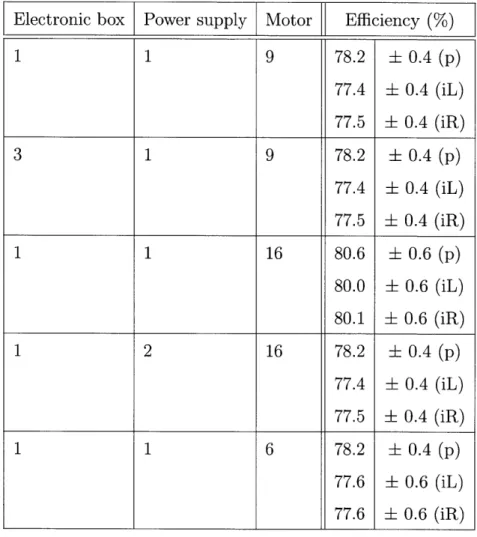
The measurements of torque described in Section 2.2 were repeated with a different electronic box, power supply, and motor. The results are presented in Table 2.2 with the mean efficiencies and uncertainties expressed in percentages. The rightmost column shows the 95% confidence interval for each efficiency. The initial electronic box, power supply, and motor used were electronic box 1, power supply 1, and motor

6; the second set of experiments were conducted with electronic box 3, power supply

2, and motors 6, 9, and 16. For a given motor and power supply, the efficiency does not depend on the electronic box. However, when the power supply was replaced, the efficiency changed by 2.6% points, about four times the measurement uncertainty of

0.6% points. To avoid changes in efficiency due to the different power supply, each

motor used during the Langley tests was calibrated using the same power supply as the one it was connected to at Langley. The effect of electronic box was negligible,

and all calibration tests used electronic box 1.

6_{The load cell should in theory measures the same value for the same loading: the average force}

(46)

Table 2.2: Summary of motor efficiencies at simulated cruise conditions: (p) for non-BLI, (iL) for left BLI propulsor, and (iR) for right BLI propulsor

Electronic box Power supply Motor Efficiency

(%)

1 1 9 78.2 t0.4 (p) 77.4 t 0.4 (iL) 77.5 0.4 (iR) 3 1 9 78.2

+0.4

(p) 77.4 t 0.4 (iL) 77.5 t 0.4 (iR) 1 1 16 80.6 t 0.6 (p) 80.0 0.6 (iL) 80.1 0.6 (iR) 1 2 16 78.2 t 0.4 (p) 77.4 0.4 (iL) 77.5 + 0.4 (iR) 1 1 6 78.2 0.4 (p) 77.6 0.6 (iL) 77.6 0.6 (iR)

2.4 Motor Efficiency Uncertainty Analysis

There are two types of uncertainties, or experimental errors, in any measured quanti-ties

[15]:

(i) random errors, such as electronic noise, and (ii) systematic errors, such as calibration errors or varying flow conditions. While the actual systematic error cannot be known, the experimental repeatability measures the combined uncertainty of the variations in systematic error plus instrumentation uncertainty (this latter is a subset

(47)

of the random error). Discussion of measurement repeatability is presented in Sec-tion 2.4.1 using a statistical approach for the evaluaSec-tion of uncertainty. SecSec-tion 2.4.2 gives the instrumentation uncertainties and describes how they are propagated to the quantity of interest: motor efficiency, %,. The instrument uncertainty includes only the random uncertainties of the measurement devices.

2.4.1 Statistical Approach for Motor Efficiency:

Measure-ment Repeatability

One way to estimate measurement uncertainty is through experiment repetition. The standard deviation gives information on the spread of the measurements, repeated N times, at the same experimental conditions. The efficiency uncertainty is based on a

95% confidence interval (oz 0.05) for an average quantity using the t-distribution

with standard deviation, S7M [16]. The efficiency is thus written as

7lm S

T -- M (2.2)

in which i is the mean value, t1-2(N-1) is the t-distribution correction factor, and

N = 4 since four runs were performed at each condition. The Shapiro-Wilk test [17]

performed for these four values for each combination of motor speed and propeller indicates that the hypothesis of normally distributed values cannot be rejected and it is appropriate to use the above t-distribution for the confidence interval.

Figure 2-6(a) shows efficiency versus RPM for the 10x08 propeller for motor 6. Black crosses represent the mean efficiencies, and the red line is a polynomial fit of order 5 of the efficiencies (chosen to best fit the data). Each point has an uncertainty error bar associated with it based on Equation (2.2) with magnitudes specified in Figure 2-6. The region of interest is shown with expanded scale in Figure 2-6(b). The error bars are 0.8% maximum of the absolute value with a 95% confidence. The results are summarized in Table 2.3 for the simulated cruise conditions for both motors 6

(48)

2000 4000 6000 8000

Q (RPM)

10000 12000 14000

(a) Full range

0.006 0.008 0.011 0.011 0.008 0.004 o.ooa 0.013 0.011 0.021 2000 4000 6000 8000 Q (RPM) 10000 12000 14000

(b) Expanded view of region of interest

Figure 2-6: Polynomial fit of the mean efficiency with uncertainty error bars (elec-tronic box 1, power supply 1, motor 6)

Table 2.3: Efficiency values at simulated cruise conditions for electronic box 1 and motors 6 and 7 with repeatability uncertainty at 95% confidence interval

Configuration Q (RPM) PE (W) 77m (%) Uncertainty (% point)

Non-BLI (left propulsor) 11600 690 78.2 + 0.4

Non-BLI (right propulsor) 11600 690 78.3 0.4

BLI (left propulsor) 11200 630 77.7 0.6

fLI (right propulsor) 11200 680 77.6 0.6

0.006 000 .6 0.011 0008 0.011 0.9- 0.8- 0.7- 0.6- 0.5- 0.4-03 0.2 -0.1 0 Cl R~. 0.8- 0.75-6 0.7- 0.65- 0.6- 0.55-0

Aerodynamic benefits of boundary layer ingestion for the D8 double-bubble aircraft

Aerodynamic Benefits of Boundary Layer Ingestion for the

D8 Double-Bubble Aircraft

Cecile

J. Casses

@

ARCHIES

OCT 14 2015

LIBRARIES

Signature redacted

Signature redacted

Signature redacted

Signature redacted

Aerodynamic Benefits of Boundary Layer Ingestion for the

D8 Double-Bubble Aircraft

Abstract

Acknowledgments

Contents

List of Figures

[5].

List of Tables

Nomenclature

Latin Letters

Q

Greek Letters

#

Superscripts

( )'

Subscripts

(

( )

(

(

(

(

(

(

(

Other Symbols

Abbreviations

Chapter 1

Introduction

1.1

The D8 Aircraft Concept

[5].

a

[5].

-1.2

Boundary Layer Ingestion

[9]

Non-BLI

BLI

1.3

NASA Langley Experiments

1.4

Thesis Goals, Contributions, and Outline

Chapter 2

Motor Calibration Experiments

#

2.1

Experimental Methodology

2.1.1

Setup

Q,

2.1.2

Data Acquisition

I

M5

Kn

1IT-1 FTI

2.1.3

Data Collection

I0

2.2

Motor Experiments Results

[5].

i

2.3

Sensitivity of Motor Efficiency to Testing

Pa-rameters