HAL Id: hal-02566581
https://hal.archives-ouvertes.fr/hal-02566581
Submitted on 7 May 2020
HAL is a multi-disciplinary open access
archive for the deposit and dissemination of sci-entific research documents, whether they are pub-lished or not. The documents may come from teaching and research institutions in France or abroad, or from public or private research centers.
L’archive ouverte pluridisciplinaire HAL, est destinée au dépôt et à la diffusion de documents scientifiques de niveau recherche, publiés ou non, émanant des établissements d’enseignement et de recherche français ou étrangers, des laboratoires publics ou privés.
UAV-based canopy textures assess changes in forest
structure from long-term degradation
Clément Bourgoin, Julie Betbeder, Pierre Couteron, Lilian Blanc, Hélène
Dessard, Johan Oszwald, Renan Le Roux, Louis Reymondin, Lucas Mazzei,
Plinio Sist, et al.
To cite this version:
Clément Bourgoin, Julie Betbeder, Pierre Couteron, Lilian Blanc, Hélène Dessard, et al.. UAV-based canopy textures assess changes in forest structure from long-term degradation. Ecological Indicators, Elsevier, 2020, 115, pp.106386. �10.1016/j.ecolind.2020.106386�. �hal-02566581�
1
UAV-based canopy textures assess changes in forest structure from long-term degradation
1
Clément Bourgoin1,2,3*, Julie Betbeder1,2,4, Pierre Couteron5, Lilian Blanc1,2, Hélène Dessard1,2, Johan
2
Oszwald6, Renan Le Roux1,2, Guillaume Cornu1,2, Louis Reymondin3, Lucas Mazzei7, Plinio Sist1,2, Peter
3
Läderach3 and Valéry Gond1,2
4
1 CIRAD, Forêts et Sociétés, F-34398 Montpellier, France
5
2 Forêts et Sociétés, Univ Montpellier, CIRAD, Montpellier, France.
6
3 International Center for Tropical Agriculture (CIAT), Hanoi, Vietnam
7
4 Ecosystems Modelling Unity, Forests, Biodiversity and Climate Change Program, Tropical Agricultural
8
Research and Higher Education Center (CATIE), Turrialba, Cartago, Costa Rica 9
5 UMR AMAP-IRD, Montpellier, France
10
6 UMR CNRS LETG 6554, Laboratory of Geography and Remote Sensing COSTEL, Université de Rennes 2
11
7 EMBRAPA Amazônia Oriental, Trav. Dr. Enéas Pinheiro, Bairro Marco, CEP, 66095-903 Belém, Pará, Brazil
12
* Correspondance: Clément Bourgoin,Campus International de Baillarguet, TA C-105/D 13
34398 Montpellier Cedex 5. E-mail : [email protected] 14
15
Abstract:
16
Degraded tropical forests dominate agricultural frontiers and their management is becoming an 17
urgent priority. This calls for a better understanding of the different forest cover states and cost-18
efficient techniques to quantify the impact of degradation on forest structure. Canopy texture 19
analyses based on Very High Spatial Resolution (VHSR) optical imagery provide proxies to assess forest 20
structures but the mechanisms linking them with degradation have rarely been investigated. To 21
address this gap, we used a lightweight Unmanned Aerial Vehicle (UAV) to map 739 ha of degraded 22
forests and acquire both canopy VHSR images and height model. Thirty-three years of degradation 23
history from Landsat archives allowed us to sample 40 plots in undisturbed, logged, over-logged and 24
burned and regrowth forests in tropical forested landscapes (Paragominas, Pará, Brazil). Fourier 25
(FOTO) and lacunarity textures were used to assess forest canopy structure and to build a typology 26
2 linking degradation history and current states. Texture metrics capture canopy grain, heterogeneity 27
and openness gradients and correlate with forest structure variability (R2= 0.58). Similar structures 28
share common degradation history and can be discriminated on the basis of canopy texture alone 29
(accuracy = 55%). Over-logging causes a lowering in forest height, which brings homogeneous textures 30
and of finer grain. We identified the major changes in structures due to fire following logging which 31
changes heterogeneous and intermediate grain into coarse textures. Our findings highlight the 32
potential of canopy texture metrics to characterize degraded forests and thus be used as indicators 33
for forest management and degradation mitigation. Inexpensive and agile UAV open promising 34
perspectives at the interface between field inventory and satellite characterization of forest structure 35
using texture metrics. 36
Highlights:
37
• We assessed canopy texture – structure relations along forest degradation gradients 38
• Canopy textures capture 58% of degradation-induced variability of canopy structure 39
• Degradation generates specific canopy textures linked with logging and fire history 40
• Texture metrics can be used to evaluate the state of degraded forests 41
42 43
Keywords:
Canopy structure, Forest degradation, Remote Sensing, Texture, Tropical forest, 44Unmanned Aerial Vehicle. 45
3
1. Introduction
47
Forest degradation is a threat (Potapov et al., 2017) to the provision of ecosystem services by tropical 48
forests. Degradation causes loss of biodiversity through habitat disturbance and fragmentation 49
(Barlow et al., 2016; Broadbent et al., 2008), erosion of hydrological and soil properties, the reduction 50
of non-timber forest resources (Lewis et al., 2015; Thompson et al., 2009), and currently accounts for 51
68.9% of overall carbon losses from tropical forests (Baccini et al., 2017). 52
The accumulation of forest disturbances such as selective logging and understory fires affects the 53
states of the forest by destroying the canopy and the internal structure without triggering any changes 54
in land use (Ghazoul and Chazdon, 2017; Putz and Redford, 2010). Degraded forests are therefore the 55
consequence of complex degradation and recovery processes, which creates a gradient of varying 56
structures within the forest landscape (Chazdon et al., 2016; Malhi et al., 2014). 57
Measuring the current forest structure and its degree of degradation are crucial for effective but 58
sustainable management of degraded forests to guarantee the conservation, management and 59
betterment of their ecological values (Goldstein, 2014). 60
However, the identification, characterization and measurement of forest degradation remains a 61
scientific challenge, in particular in the remote sensing community (Frolking et al., 2009; Herold et al., 62
2011; Hirschmugl et al., 2017; Mitchell et al., 2017). Among the wide range of remote sensing 63
approaches, optical time series of medium resolution Landsat images have been used to derive forest 64
states indicators and to reconstruct forest degradation history through the detection and 65
quantification of disturbances within the canopy (Asner et al., 2009; Bullock et al., 2018; DeVries et 66
al., 2015; Souza et al., 2013). These approaches are steps towards degradation monitoring and 67
informing Reducing Emissions from Deforestation and Degradation (REDD+) systems (Goetz et al., 68
2014) but do not provide quantitative information on the forest structure which is directly related to 69
carbon stocks. Airborne Light Detection and Ranging (A-LiDAR) is the most successful technique to 70
retrieve three-dimensional forest structural parameters and estimate aboveground biomass (AGB) 71
4 stocks (Asner et al., 2012; Longo et al., 2016; Rappaport et al., 2018) but the data are often costly to 72
acquire and to replicate both in space and over time (Silva et al., 2017). 73
In addition to the spectral properties of optical remote sensing, Very High Spatial Resolution (VHSR) 74
sensors (images with less than 5m/pixel) also acquire information on the distribution of dominant tree 75
crowns that define the forest canopy and also canopy gaps, thereby providing important indirect 76
indicators of forest three-dimensional structure (Meyer et al., 2018). The spatial distribution of trees, 77
the shapes and dimensions of their crowns and the characteristics of the inter-crown gaps interact to 78
define the forest canopy grain and can be assessed through canopy texture analysis (Couteron et al., 79
2005). Several studies have demonstrated the potential of texture methods to characterize VHSR 80
canopy images (Couteron et al., 2005; Frazer et al., 2005). Among them, the FOurier-based Textural 81
Ordination (FOTO) method has been used in a variety of tropical forests to characterize gradients of 82
canopy grain, heterogeneity and crown size distribution (Barbier et al., 2010; Bastin et al., 2014; 83
Couteron et al., 2005; Ploton et al., 2012; Singh et al., 2014). Case studies have shown that FOTO 84
indices can correlate with forest structural parameters along gradients of natural variation (Couteron 85
et al. 2005) of degradation (Ploton et al. 2012; Singh et al. 2014) or in landscapes mixing both (Bastin 86
et al. 2014 ; Pargal et al. 2017). Lacunarity analysis, another textural approach, also captures spatial 87
heterogeneity of forest canopies and additionally provides a quantitative measure of canopy 88
‘gapiness’ that correlates with canopy cover and gap fraction (Frazer et al., 2005; Malhi and Román-89
Cuesta, 2008; Ploton et al., 2017). However, the possible links between canopy texture and forest 90
structure parameters are context dependent (Ploton et al. 2017), and relationships have to be verified 91
and calibrated using reference data from either field plots or airborne canopy altimetry, and such data 92
are not available in many tropical landscapes or regions. Moreover, one cannot expect the variety of 93
stand structures generated by degradation processes to display unequivocal relationships with canopy 94
texture variables (Rappaport et al., 2018). For instance, severe degradation may result in coarse 95
texture (e.g. because of big gaps) as well as fine-grained aspects owing to small crowns in regenerating 96
patches. In this sense, there is a lack in understanding and quantifying the consequences of forest 97
5 degradation on canopy texture. Using unmanned aerial vehicles (UAV), the aim of this paper is to 98
demonstrate that texture information can efficiently characterize degraded forest types. Unmanned 99
aerial vehicles are thus a new promising tool to acquire altimetry data and very high resolution images 100
of the canopy (Koh and Wich, 2012; Zhang et al., 2016). 101
Here, we used very high resolution UAV images to sample a broad range of degraded and intact forests 102
conditions in an old deforestation pioneer front of the Brazilian Amazon. For each forest site, we 103
combined degradation history from Landsat time series with UAV data including canopy elevation and 104
grey-level images. Our large-area and diverse UAV coverage addressed two questions: (1) How do 105
canopy textures correlate with forest structure parameters within a large range of degraded forest 106
types? (2) How do disturbance type and frequency contribute to variability in texture metrics through 107
heterogeneity, coarseness and openness canopy gradients? 108
In so doing, our study aims to pave the way for interpreting canopy texture in VHSR satellite images 109
from agile UAV-based ground truthing and consequently help decision makers improve the 110
management of degraded forests. 111 112 113 114 115 116
6
2. Materials and Methods
117
2.1. Study area 118
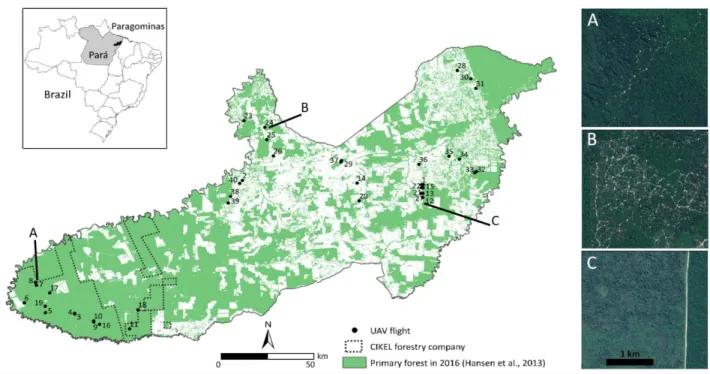
The study was carried out in the municipality of Paragominas, located in the northeastern part of the 119
State of Pará, Brazil, and covered an area of 19,342 km² (Fig. 1). The municipality experienced different 120
colonization processes since its foundation in 1965, which led to significant deforestation with 121
conversion of land to pasture for cattle ranching and forest degradation through overexploitation of 122
timber. Deforestation was accentuated by the grain agro-industry in the 2000s, dominated by 123
intensive soybean and maize cultivation mainly in the center of the municipality (Piketty et al., 2015). 124
We demonstrated in previous studies that the history and processes of colonization spatially differ 125
within Paragominas (Laurent et al., 2017). This led to a mosaic of forests in very different cover states 126
within heterogeneous landscape mosaics dominated by different land uses (Bourgoin et al., 2018; 127
Mercier et al., 2019). In this region, forest management plans with selective logging have rarely been 128
adopted except in CIKEL Brasil Verde Madeiras Ltda forestry company (Mazzei et al., 2010). Forest 129
suffered from two major anthropogenic disturbances. Unplanned logging with over-logging intensity 130
is marked by repeated frequencies over time. Fire alters deeply the understory and generate high 131
mortality rates for canopy trees (Fig. 1)(Hasan et al., 2019; Tritsch et al., 2016). 132
7 133
Figure 1: Location of the study site, Paragominas municipality, in Pará state in the Brazilian Amazon. Distribution of the 40
134
forest plots covered using UAV. Illustrations of selective logging (A), over-logging (B) and fire (C) from Google Earth® 2017
135
2.2. Data collection 136
2.2.1. UAV surveys and processing 137
Forty forest sites were selected in various forested landscapes to cover a large variation of disturbance 138
types (Fig.1). Using visual interpretation from Google Earth® VHSR images validated by in-situ UAV 139
observations, we distinguished between sites that experienced disturbances such as logging and fire 140
and intact sites with no human-induced disturbance. We also used the management plan of the Cikel 141
forestry company (Fig.1) that provides spatial information on undisturbed and selectively logged 142
forests at different dates over the last 20 years. 143
We used a DJI mavic pro UAV carrying its original RGB camera of 12.71 megapixel resolution (DJI, 144
Shenzhen, China). The acquisition plan was designed with Pix4D Capture software (Pix4D, Lausanne, 145
Switzerland). We used a single grid with 80% of front and side overlap between images and a constant 146
flight altitude of 300 meters above ground level. The objective was to maximize the overlap between 147
each image and the total surface area mapped. As a result, the average surface mapped in each forest 148
plot was 24 ha (~600 by 400 meters) at 10 centimeters spatial resolution (Appendix C) for a total of 149
8 739 ha. In order to generate a high quality canopy height model, each flight was constrained by several 150
conditions: 151
i) Flat terrain was selected with imaged areas that overlapped with roads or agricultural fields 152
to allow us to retrieve the ground elevation during the preprocessing step; 153
ii) Acquisition in the morning (9 to 11 am) and afternoon (3 to 5 pm) was preferred to avoid 154
zenithal effects (halo and low image contrast); 155
iii) Either cloud free or totally cloudy sky conditions were necessary to avoid cloud shadows; 156
iv) Absence of wind to low wind conditions were needed to generate crisp images of the forest 157
canopy. 158
Raw image data were processed to the highest density point cloud using structure from motion (SfM) 159
followed by densification using multi-view stereo algorithms in the Pix4D software (Alonzo et al., 2018; 160
Westoby et al., 2012). Final point cloud densities were ~27 pts.m-3 depending on the availability of 161
viable tie points, and some other acquisition parameters (Table 1). Using the georectified point clouds, 162
we corrected the raw images to generate RGB mosaics, which were then converted into single-band 163
panchromatic grey level mosaics. Digital Surface Models (DSM) of the canopy (i.e. the top of the 164
forest’s surface) at 0.10 m resolution were directly computed from the point cloud. We extracted the 165
average ground elevation data in non-forest areas (e.g. roads, agricultural fields or canopy gaps) from 166
the DSMs and derived canopy height models for each forest plot. 167
168
2.2.2. Landsat time series to detect forest disturbances and reconstruct degradation history 169
We acquired Landsat data from 1984 to 2017 (Appendix A) to detect forest disturbances along time 170
and reconstruct degradation history for each forest site. The images at Level 1 (Tier 1 product) were 171
pre-processed to surface reflectance by the algorithm developed by the NASA Goddard Space Flight 172
Center (http://earthexplorer.usgs.gov/). We computed the Normalized Difference Moisture Index 173
9 (NDMI) from the Short-Wave InfraRed (SWIR) and Near InfraRed (NIR) bands as follows (Gao, 1996): 174
𝑁𝐷𝑀𝐼 = 𝑁𝐼𝑅 − 𝑆𝑊𝐼𝑅 𝑁𝐼𝑅 + 𝑆𝑊𝐼𝑅⁄ 175
This index previously used to monitor forest degradation (DeVries et al., 2015) allowed us to identify 176
disturbance type and frequency (selective logging, over-logging and fire) at forest plot scale, using 177
photointerpretation (Appendix B). The disturbance type was identified based on its spatial extent and 178
shape and on the low NDMI values. Selective logging is marked by regular and spaced logging roads 179
(Fig.1A), over-logging is marked by irregular logging roads (Fig. 1B) and fire presents open canopy 180
structure and low values of NDMI (Silva et al., 2018; Tritsch et al., 2016). We also recorded the date of 181
the most recent disturbance (Appendix C) which has a significant influence on the current forest 182
structure (Rappaport et al., 2018). Figure 2 shows the diversity of forest degradation history of our 183
sampling such as selectively logged forests, over-logged forests and over-logged and burned forests. 184
185 186
Figure 2: Forest degradation history of the 40 forest plots based on the frequency of selective logging, 187
over-logging, fire events and date of last disturbance (4 plots are not shown as they are secondary 188
forests). 189
2.3. Methods
190
The data analysis was based on two steps: (1) use canopy texture metrics derived from grey-level UAV 191
images to retrieve canopy structure metrics (based on canopy height models) derived from UAV 192 1992 1997 2002 2007 2012 2017 0 1 2 3 4 5 6 D is tur ba nc e fr equenc y Forest plots
10 structure from motion within a large range of degraded forest types at 1 ha scale and (2) potential of 193
canopy texture metrics to discriminate degradation history and the resulting changes in forest 194
structures at the forest plot scale (Fig. 3). 195
196
Figure 3: Workflow of the method used to evaluate the potential of canopy texture metrics to retrieve 197
the canopy structure along the gradient of forest degradation and their relation with forest 198
degradation history. 199
200
2.3.1. Computation of forest canopy texture metrics from grey level UAV images at 1 ha scale 201
We performed texture analysis of grey level canopy images using FOTO (Couteron, 2002) and 202
lacunarity (Frazer et al., 2005) algorithms. We also used basic descriptors of statistical grey level 203
distributions such as skewness and kurtosis. Each of the UAV canopy images was divided into canopy 204
100*100 m windows (fixed grid) for texture analysis. This size was shown in previous studies to be 205
11 appropriate to capture several repetitions of the largest tree crowns (in our case 45 meters of 206
maximum tree crown diameter) in forest stands (Ploton et al., 2017). 207
The FOTO method is extensively described elsewhere (Couteron, 2002; Couteron et al., 2005; Ploton 208
et al., 2017), hence we only give here a brief outline of the procedure. When applying FOTO, each of 209
the windows originating from the UAV images is subjected to a two-dimensional Fourier transform to 210
enable computation of the two-dimensional periodogram. ‘Radial-’ or ‘r-spectra’ are extracted from 211
the periodogram to provide simplified, azimuthally-averaged textural characterization. Spectra are 212
systematically compared using the two first axes of a principal component analysis (FOTO_PCA1, 213
FOTO_PCA2), providing an ordination along a limited number of coarseness vs. fineness gradients. In 214
this process, windows are treated as statistical observations that are characterized and compared on 215
the basis of their spectral profile, i.e., the way in which window grey scale variance is broken down in 216
relation to Fourier harmonic spatial frequencies (ranging from 50 to 240 cycles/km for this study). PCA 217
captures gradients of variation between windows spectra opposing those concentrating most variance 218
in low frequencies (i.e. coarse textures) and those in which high frequencies retain a substantial share 219
of variance (i.e. fine textures). 220
221
Lacunarity was defined following Frazer et al. (2005) and Malhi and Roman-Cuesta (2008). For each 222
100*100 m window, a moving square box of size ‘s’ was glided by one pixel at a time and the sum of 223
all pixel spectral radiance, called the mass, was computed at each gliding position. The frequency 224
distribution of the mass divided by the number of boxes’ positions is computed, and Lacunarity at box 225
size ‘s’ is the squared ratio of the first and second moment of this distribution. This process was 226
repeated for 100 box sizes ranging from 1 to 99 m and the resulting lacunarity spectrum was 227
normalized by lacunarity at size 1. Finally, the spectra were compared using the two first axes of a PCA 228
(Lacu_PCA1 and Lacu_PCA2 respectively), to provide an ordination of windows along inter-crown 229
canopy openness gradients. 230
12 Routines for both FOTO (http://doi.org/10.5281/zenodo.1216005) and lacunarity methods were 231
developed in the MatLab® environment (The MathWorks, Inc., Natick, Massachusetts, USA). 232
233
2.3.2. Computation of forest canopy structure metrics from canopy height models at 1 ha scale 234
From the canopy height model, six Canopy Structure Metrics (CSM) were computed in the same 235
100*100m window grid previously described: mean elevation (mean), minimum (min), maximum 236
(max), variance (var), Standard Deviation (SD) and Coefficient of Variation (CV) defined as the ratio 237
between standard deviation and mean elevation. We then compiled the six Canopy Texture Metrics, 238
noted CTM, (FOTO_PCA1, FOTO_PCA2, Lacu_PCA1, Lacu_PCA2, Skewness, Kurtosis) and the 6 CSM. 239
240
2.3.3. Canopy texture - structure relations within a large range of degraded forest types at 1 ha scale 241
The ability of CTM to predict forest canopy structures was tested using regression models for each 242
CSM based on Random Forest machine learning (RF) (Breiman, 2001). 243
The learning set is randomly partitioned into k equal size sub-samples with k=10. Each regression 244
process is then applied where k-1 sub samples are used as training data and the remaining ones for 245
validation. This process is repeated by changing the training/validation sub-samples in such a way that 246
all learning samples are used for validation. Cross-validation is a common and sound procedure in 247
machine learning processes (Arlot and Celisse, 2010; Kohavi, 1995). The R-squared, average Root 248
Mean Square Error (RMSE) and relative RMSE were utilized to evaluate the performance of the model. 249
The number of trees and the number of variables used for tree nodes splitting were randomly 250
determined using the tune function implemented in the R randomForest package, version 4.6-14 (Liaw 251
and Wiener, 2002). The number of tree was set to 500 to reduce computation times without notable 252
loss in accuracy. 253
254
2.3.4. Potential of canopy texture metrics to discriminate forest degradation histories at the plot scale 255
13 The forest plot scale was used to combine canopy texture and canopy structure metrics with forest 256
degradation history. We first classified forest plots according to their canopy structures (mean CSM 257
calculated at the plot scale) using PCA and hierarchical clustering (Ward’s criterion). The number of 258
clusters was optimized by calculating the inter-cluster variance (Ketchen Jr. and Shook, 1996). Each 259
cluster of forest canopy structure was then related to forest degradation history by calculating the 260
average disturbance frequency of over-logging, selective logging and fire events. We then used Linear 261
Discriminant Analysis (LDA) to predict membership of forest structure clusters from averaged value of 262
CTM at the plot scale. LDA algorithm tries to find a linear combination within the canopy textural 263
metrics averaged at plot scale that maximizes separation between the barycenters of the clusters 264
while minimizing the variation within each group of the dataset (Hamsici and Martinez, 2008; Kuhn 265
and Johnson, 2013). We used MANOVA with Pillai’s Trace tests to evaluate the significance of the 266
multivariate inter-cluster difference computed from the 6 CTM. All processes were computed using 267
the R packages FactoMineR (Husson et al., 2010; Lê et al., 2008) and the MASS package (Venables and 268 Ripley, 2002). 269 270
3. Results
2713.1. Forest canopy texture metrics from grey level UAV images at 1 ha scale
272
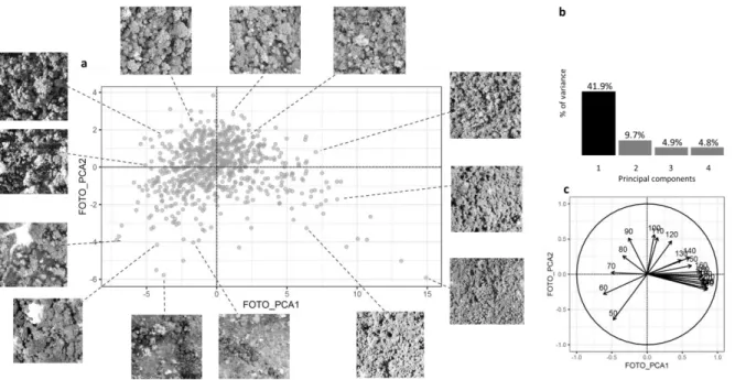
The two first factorial axes of the PCA accounted for 51.6% of the total variability of the r-spectra 273
observed (Fig. 4b). FOTO_PCA1 expresses a gradient between coarse and fine texture corresponding 274
to spatial frequencies of less than 90 cycles/km and more than 120 cycles/km, respectively (Fig. 4c). 275
FOTO_PCA2 expresses a gradient leading from heterogeneous textures with the coexistence of low 276
and high frequencies (negative scores) toward homogeneous intermediate frequencies in the range 277
90-120 cycles/km (high scores). Fine textures correspond to homogeneous distribution of small tree 278
crowns reflecting ongoing regeneration after probable over-logging. Intermediate textures along axis 279
1 associate large and smaller tree crowns that characterize preserved forest with the natural 280
distribution of high emergent trees and lower canopy trees. The left part of the scatter plot groups 281
14 coarse textures corresponding to large gaps in the canopy related to logging activities. Finally, the two 282
examples at the bottom of the plot show mixed coarse (remaining trees) and fine (low understory or 283
shrub stratum) textures that characterize over-logged and recently burned forests. 284
285
286
Figure 4: Canopy texture ordination based on the FOTO method applied to UAV-acquired grey level images. (a) Scatter plots
287
of PCA scores along F1 and F2 and windows selected as illustrations. (b) Histogram of eigenvalues expressed as % of total
288
variance. (c) Correlation circles with frequencies ranging from 50 to 240 (cycles/km).
289
The first factorial axe of the PCA on the lacunarity spectra account for more than 70% of total 290
variability (Fig. 5b). Lacu_PCA1 expresses a gradient of gapiness with large gaps appearing in the 291
extreme left part of the scatter plot (Fig. 5a) and closed canopy forest with no gaps in the extreme 292
right part. Large gaps are tree shadows projected over large canopy gaps. Homogeneous canopies, i.e. 293
smooth grain and a closed canopy characterizing low degradation forests were found on the positive 294
side of the second axis (Lacu_PCA2)(11% of total variability) and vice versa for heterogeneous 295
canopies. These are highly degraded forests (over-logged at different ages and recently burned 296
forests) with destroyed canopies and patches of small crowns linked to the understory or to 297
regeneration. Other axes did not reveal other structures. Substantial analogy can be observed 298
between the main texture gradients provided by FOTO and by the lacunarity analyses. 299
15 300
Figure 5: Canopy texture ordination based on the lacunarity method. (a) Scatter plots of PCA scores along F1 and F2 and
301
windows selected as illustrations. (b) Histogram of eigenvalues expressed as % of total variance. (c) Correlation circles with
302
sub-window sizes ranging from 2 to 102 pixels.
303
3.2. Relationships between canopy textures and forest structure parameters at 1 ha scale
304
The standard deviation and variance of canopy height were the CSM best explained by texture with a 305
R² of 0.58 and 0.54 respectively (Table 1). These metrics pointing to the variability of canopy structure 306
directly reflect the different processes of degradation and the associated gradients of canopy grain 307
texture. Maximum and mean canopy height and coefficient of variation show lower relationship (resp. 308
R² of 0.43, 0.38 and 0.31). The minimum height showed a low R² of 0.13 with CTM. 309
Table 1: Random forest regression models for the prediction of canopy structure metrics (CSM) from canopy texture metrics
310
(CTM) on grey level images.
311
CSM R² RMSE Relative RMSE
Minimum (m) 0.13 3.49 0.94
Maximum (m) 0.43 5.66 0.76
Mean (m) 0.38 4.88 0.79
16
Standard deviation 0.58 1.01 0.65
Coefficient of variation 0.31 0.17 0.83
312
3.3. Potential of canopy texture metrics to discriminate forest degradation histories at the plot scale
313
3.3.1. Clusters of canopy structures and related degradation history 314
The clustering method allowed identifying six clusters of canopy structures (Fig. 6). Cluster 1 groups 315
wide open and low canopy forests with a significantly lower average canopy height (9.9 m) than the 316
other clusters and high Standard Deviation (SD) values (6.19 m). It groups forest plots that have mainly 317
experienced over-logging (~1.4 events) and recent fire events identified between 2015 and 2017 (1.6 318
in average). Cluster 2 groups 23-year-old secondary forests characterized by a homogeneous and low 319
canopy (average height of 13.86m and SD of 2.28). Cluster 3 groups forest plots with homogeneous 320
(SD of 5.10), low average canopy height (14.13m) mainly marked by over-logging (~1.5 events). Cluster 321
4 has a heterogeneous canopy structure characterized by high standard deviation (SD of 7.03) which
322
is explained by recent logging events detected in 2017 (~1.2 events) and other previous disturbances 323
such as fire (~1 event). Clusters 5 and 6 have similar canopy height (~22 m) but variable canopy 324
roughness (SD ranging from 6.05 to 7.59). Their degradation histories differ as cluster 5 groups 325
recently selectively logged forest (~0.6 events) or over-logged forests (~1 event) while cluster 6 mostly 326
groups undisturbed forest and old selectively logged forests (more than 10 years ago). However both 327
clusters are marked by very low (~0.1 events for cluster 5) to none fire disturbances detected. Further 328
explanation on the different steps of the method and on the statistical results can be found in 329
Appendix D and E. 330
17 331
Figure 6: Three-dimensional plots of canopy height models of the 100 x 100 m windows selected to illustrate the six forest
332
structure clusters. Radar chart shows the average frequency of over-logging, selective logging and fire disturbances detected
333
in all forest plots within a given cluster.
334
335
3.4.2. Linear discriminant analysis at the forest plot scale 336
The two first discriminant components (LD1 and LD2) account for 93.6% of the total proportion of the 337
trace i.e. the proportion of inter-cluster discrimination of the LDA based on texture (MANOVA test 338
with p-value < 0.05)(Fig. 7a). The prominent first discriminant component is mainly correlated with 339
FOTO_PCA1 (r=0.55 in LD1), FOTO_PCA2 (0.49 in LD1) and LACU_PCA2 (-0.79 in LD1) (Fig. 7b). The 340
second discriminant component is mainly correlated with LACU_PCA2. 341
In the LD1-LD2 plane, clusters 2 and 3 are mainly separated from the rest of clusters thanks to axis 342
LDA1. Cluster 1, 4 and 5 are discriminated along LD2. Cluster 6 has less discriminating capacity, 343
especially compared with cluster 5. 344
LDA results include misclassification errors corresponding to disagreement between texture-based 345
and structural classifications of the plots (Fig. 7a). The confusion matrix shows an overall accuracy of 346
55% and kappa index at 0.44 (Fig 7c). The LDA classification performed well for all clusters except 347
18 cluster 6 which has the highest misclassification rate with a high rate of confusion with cluster 5. Based 348
on CTM, clusters 5 and 6 appeared to be similar because they mainly differ in their minimum height, 349
which logically is difficult to predict from canopy texture metrics on 2D images. 350
351
352
Figure 7: (a) Scatter plot showing the distribution of the 40 forest plots with color based on the color of canopy clusters on
353
the linear discriminant plane (LD1-2). Inset: proportions of LDA trace (b) Correlation circle of CTM with respect to the two
354
main components (axes) of the LDA (c) Confusion matrix between observed and predicted clusters for the 40 plots (LDA
355
classifications)
356
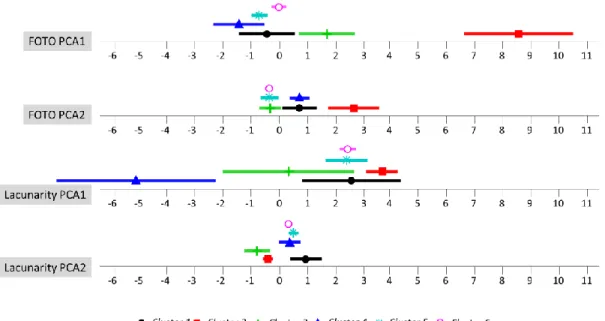
Clusters 2, 3 and 5 are distinguished along a gradient of canopy textural grain that spans from fine to 357
coarse (FOTO-PCA1) (Fig. 8). Cluster 4 mainly presents the lowest FOTO-PCA1 and Lacunarity-PCA1 358
values, which correspond to the coarse texture and large gaps, respectively, typical of recent logging 359
events. Cluster 1 has on average the coarse grain and homogeneous texture (FOTO-PCA1 and -PCA2) 360
that characterize low vegetation strata. Finally cluster 6 (well preserved forest) has intermediate 361
canopy grain (FOTO-PCA1 and 2) and canopy openness (Lacunarity-PCA2). 362
19 364
Figure 8: Mean and SD values of CTM calculated within the 6 predicted clusters using LDA.
365
366 367
20
4. Discussion
368
A better characterization of forest structure is crucial to tailoring forest management plans (Goldstein, 369
2014). In this paper, we show that canopy texture metrics extracted from very-high spatial resolution 370
optical images acquired by unmanned aerial vehicle are clearly related to forest canopy height models 371
and can reveal different and complex degradation history. The canopy texture metrics provide 372
complementary information on degraded forest states compared to other remotely sensed indicators 373
based on vegetation photosynthesis activity (Asner et al., 2009; Bullock et al., 2018; Mitchell et al., 374
2017). The canopy texture metrics can also be used in multidisciplinary approaches such as for the 375
assessment of forest ecosystem services that require detailed information on forest structure (Barlow 376
et al., 2016; Berenguer et al., 2014). 377
378
4.1. Potential of canopy texture metrics to assess degraded canopy structures
379
We showed that CTM can assess forest structure variability that reflects both horizontal and vertical 380
heterogeneity induced by degradation. Through the expression of canopy grain and heterogeneity 381
gradients, CTM provides reliable estimations of canopy roughness (standard deviation of canopy 382
height) at 1 ha-scale. At the forest plot scale, we demonstrated the complementary of FOTO and 383
lacunarity metrics in distinguishing between the different clusters. While FOTO and lacunarity express 384
similar gradients of canopy texture (Figs. 4 and 5), the measure of canopy openness in lacunarity 385
provide useful additional information to distinguish large canopy gaps from large crowns, as 386
underlined by Ploton et al. (2017). However, the first axis of lacunarity reveals a gradient of canopy 387
textures that could be influenced by sun-angle conditions during the UAV data acquisition. Early 388
morning and late afternoon data acquisitions generate higher projected shadow, which drives the 389
distribution of the data towards the negative values of the first axis. Data acquisition parameters (sun 390
and sensor angles, clouds etc.) are known to be able to disturb grey level values and textures (Barbier 391
and Couteron, 2015). One advantage of using UAV is that they allow better control of acquisition 392
conditions than do satellites. 393
21 394
4.2. Long-term forest degradation consequences on structure explained using current canopy 395
textures
396
In this study, we demonstrate the potential of single shot UAV-based canopy altimetry and texture to 397
correlate with current structure that can reveal both past disturbances and recovery processes (Herold 398
et al. 2011, Ghazoul and Chazdon 2017). At the forest plot scale (~24 ha), the average CSM and the 399
variability of CSM enabled the identification of six forest clusters with specific degradation history. The 400
link between long term degradation history and canopy structure has already been identified in 401
previous studies that quantified carbon densities of Amazonian forests following successive logging 402
and/or fire events (Berenguer et al., 2014; Longo et al., 2016; Rappaport et al., 2018). CTM proved to 403
be able to differentiate between five types of degradation, although with some confusion between 404
the less degraded forest types. 405
Undisturbed forests have a high closed canopy, and are homogeneous in texture with an intermediate 406
grain associating large and medium-sized tree crowns (cluster 6). Any logging event will disrupt the 407
canopy and create a coarse texture with greater variation in canopy height (cluster 4). Under a 408
management plan, logging intensity is moderate (< 5 to 8 trees/ha) and the recovery time (35 years in 409
Brazil) is expected. In that case, the coarse texture will recover and will turn back into intermediate 410
grain (cluster 5 or 6). We showed that after seven years, the canopy texture of a logged forest 411
resembles that of undisturbed forest (Fig. 6 and Appendix C). For unmanaged forests, subject to higher 412
uptake, the time for the forest to recover a canopy texture of intermediate grain will be longer (e.g. 413
plots 23 and 24). In the case of additional impacts (progressive disappearance of large crowns), the 414
coarse canopy texture will also be maintained longer. Repetitive and intense logging have therefore 415
triggered the complete harvesting of emergent trees, thereby weakening the capacity of forests to 416
cope with further disturbances (Asner et al., 2002). During the recovery process, canopy is of low 417
height and its texture is dominated by a fine and heterogeneous grain (cluster 3). 418
22 Additionally, we found that recent fire (single or multiple events) has a major impact on the damaged 419
forest structure. The resulting highly degraded forests are characterized by coarse textures 420
corresponding to large gaps and/or homogeneous regeneration stratum and highly damaged canopy 421
(cluster 1). Moreover, most fires were detected in 2015, which correlated with the El Nino drought 422
event (Berenguer et al., 2018). These findings underline the importance of the synergetic effects of 423
logging and fire on forest structure (Dwomoh et al., 2019; Morton et al., 2013). We also found that 424
fire was never detected (i.e. did not occur) in closed canopy and relatively low degradation forests. 425
This confirms that heavily logged forests are more vulnerable to fire due to the presence of dead and 426
dry vegetation resulting from logging. At a larger scale, this vulnerability is linked with the 427
fragmentation of forest patches, which facilitates access to forest resources, accentuates dry edge 428
effects and increases potential pressure caused by agricultural expansion (Briant et al., 2010; 429
Broadbent et al., 2008; Silva Junior et al., 2018). The mitigation of fire occurrence through improved 430
landscape management is therefore a priority in order to prevent further degradation and forest 431
carbon losses (Berenguer et al., 2014). 432
The results of the present study reveal possible ways to address questions concerning the future 433
management of primary degraded forests by analyzing the structure and texture of their canopy in 434
order to better differentiate forest states and the associated degradation history. This study also 435
opens the way for further analysis of secondary forests in abandoned lands which will certainly play a 436
crucial role in future scenarios of landscape restoration (Chazdon et al., 2016). 437
438
4.3. UAV technology: from data acquisition to limitations and perspectives
439
This paper reports the first large-scale application of low cost UAV to retrieve quantitative information 440
on closed canopy forest structures. The UAV used is inexpensive (<2,000 US$) and a highly efficient 441
cost/time ratio was found for data acquisition in the field. In a 20 minutes flight, around 25 hectares 442
of forest was mapped at a resolution of 10 centimeters. Other studies using UAV produced results that 443
are comparable with LiDAR in terms of point cloud densities (Chung et al., 2019; Dandois et al., 2015) 444
23 and estimations of forest structural parameters (Alonzo et al., 2018). Finally, the computation of CTM 445
using open-source Matlab® routines is automatic and only requires the window size used for texture 446
analysis as the user input. Window size can be adapted to forest canopy crown size and distribution, 447
although limited variations do not alter the results much. Consequently, the workflow described here 448
has great promise for future monitoring of tropical forest at low cost, which is interesting when 449
airborne LiDAR is not affordable or available. 450
However, UAV remain limited by their inability to cover regions as large as those covered by satellite 451
images, and climatic conditions (wind, cloud shadows) are likely to disturb the consistency of image 452
texture and thus the automatic mapping process. Finally, regulations strongly limit the use of UAV in 453
certain countries. Nonetheless, UAVs appears to be an efficient tool at the interface between field 454
inventory and satellite characterization of forest structure (Koh and Wich, 2012). Unmanned aerial 455
vehicle acquired reference data could be the basis of upscaling chains that would allow the use of 456
spaceborne data of decreasing resolution yet increasing swath and affordability so as to reach broad 457
scale, wall to wall mapping of forest state indicators of known accuracy. 458
459
Authors’ contributions
460
CB, JB, LB, JO, LR, PL and VG conceived the ideas and designed methodology; CB, JB, LB and VB collected 461
the data; CB, JB, PC, LB, HD, LR and VG analyzed the data; CB, PC, VG, LB and PS led the writing of the 462
manuscript. All authors contributed critically to the drafts and gave final approval for publication.
463
Acknowledgements
464
This work was supported by 1) the European Union through the H2020-MSCA-RISE-2015 ODYSSEA 465
project (Project Reference: 691053), by 2) the CNES (France) through the TOSCA CASTAFIOR project (ID 466
4310), by 3) the EIT through the Climate-KIC ForLand Restoration project and by 4) the CGIAR Research 467
Program on Forest Trees and Agroforestry (FTA) and on Climate Change, Agriculture and Food Security 468
(CCAFS), the latter with support from CGIAR Fund Donors and through bilaterial funding agreements. 469
24 For details, please visit https://ccafs.cgiar.org/donors. The views expressed in this document cannot 470
be taken to reflect the official opinions of these organizations 471
Conflicts of Interest:
The authors declare no conflict of interest. 472473
References
474
Alonzo, M., Andersen, H.-E., Morton, D., Cook, B., 2018. Quantifying Boreal Forest Structure 475
and Composition Using UAV Structure from Motion. Forests 9, 119. 476
https://doi.org/10.3390/f9030119 477
Arlot, S., Celisse, A., 2010. A survey of cross-validation procedures for model selection. 478
Statist. Surv. 4, 40–79. https://doi.org/10.1214/09-SS054 479
Asner, G.P., Keller, M., Pereira, R., Zweede, J.C., 2002. Remote sensing of selective 480
logging in Amazonia: Assessing limitations based on detailed field observations, 481
Landsat ETM+, and textural analysis. Remote Sensing of Environment 80, 483–496. 482
Asner, G.P., Knapp, D.E., Balaji, A., Páez-Acosta, G., 2009. Automated mapping of tropical 483
deforestation and forest degradation: CLASlite. Journal of Applied Remote Sensing 484
3, 033543–033543. 485
Asner, G.P., Mascaro, J., Muller-Landau, H.C., Vieilledent, G., Vaudry, R., Rasamoelina, M., 486
Hall, J.S., van Breugel, M., 2012. A universal airborne LiDAR approach for tropical 487
forest carbon mapping. Oecologia 168, 1147–1160. https://doi.org/10.1007/s00442-488
011-2165-z 489
Baccini, A., Walker, W., Carvalho, L., Farina, M., Sulla-Menashe, D., Houghton, R.A., 2017. 490
Tropical forests are a net carbon source based on aboveground measurements of 491
gain and loss. Science 358, 230–234. https://doi.org/10.1126/science.aam5962 492
Barbier, N., Couteron, P., 2015. Attenuating the bidirectional texture variation of satellite 493
images of tropical forest canopies. Remote Sensing of Environment 171, 245–260. 494
https://doi.org/10.1016/j.rse.2015.10.007 495
Barbier, N., Couteron, P., Proisy, C., Malhi, Y., Gastellu-Etchegorry, J.-P., 2010. The 496
variation of apparent crown size and canopy heterogeneity across lowland 497
Amazonian forests: Amazon forest canopy properties. Global Ecology and 498
Biogeography 19, 72–84. https://doi.org/10.1111/j.1466-8238.2009.00493.x 499
Barlow, J., Lennox, G.D., Ferreira, J., Berenguer, E., Lees, A.C., Nally, R.M., Thomson, J.R., 500
Ferraz, S.F. de B., Louzada, J., Oliveira, V.H.F., Parry, L., Ribeiro de Castro Solar, 501
R., Vieira, I.C.G., Aragão, L.E.O.C., Begotti, R.A., Braga, R.F., Cardoso, T.M., Jr, 502
R.C. de O., Souza Jr, C.M., Moura, N.G., Nunes, S.S., Siqueira, J.V., Pardini, R., 503
Silveira, J.M., Vaz-de-Mello, F.Z., Veiga, R.C.S., Venturieri, A., Gardner, T.A., 2016. 504
Anthropogenic disturbance in tropical forests can double biodiversity loss from 505
deforestation. Nature 535, 144–147. https://doi.org/10.1038/nature18326 506
Bastin, J.-F., Barbier, N., Couteron, P., Adams, B., Shapiro, A., Bogaert, J., De Cannière, C., 507
2014. Aboveground biomass mapping of African forest mosaics using canopy texture 508
analysis: toward a regional approach. Ecological applications 24, 1984–2001. 509
Berenguer, E., Ferreira, J., Gardner, T.A., Aragão, L.E.O.C., De Camargo, P.B., Cerri, C.E., 510
Durigan, M., Oliveira, R.C.D., Vieira, I.C.G., Barlow, J., 2014. A large-scale field 511
assessment of carbon stocks in human-modified tropical forests. Global Change 512
Biology 20, 3713–3726. https://doi.org/10.1111/gcb.12627 513
Berenguer, E., Malhi, Y., Brando, P., Cardoso, A., Cordeiro, N., Ferreira, J., Franca, F., 514
Rossi, L.C., 2018. Tree growth and stem carbon accumulation in human-modified 515
Amazonian forests following drought and fire 8. 516
25 Bourgoin, C., Blanc, L., Bailly, J.-S., Cornu, G., Berenguer, E., Oszwald, J., Tritsch, I.,
517
Laurent, F., Hasan, A.F., Sist, P., Gond, V., 2018. The Potential of Multisource 518
Remote Sensing for Mapping the Biomass of a Degraded Amazonian Forest 21. 519
Breiman, L., 2001. Random forests. Machine learning 45, 5–32. 520
Briant, G., Gond, V., Laurance, S.G.W., 2010. Habitat fragmentation and the desiccation of 521
forest canopies: A case study from eastern Amazonia. Biological Conservation 143, 522
2763–2769. https://doi.org/10.1016/j.biocon.2010.07.024 523
Broadbent, E., Asner, G., Keller, M., Knapp, D., Oliveira, P., Silva, J., 2008. Forest 524
fragmentation and edge effects from deforestation and selective logging in the 525
Brazilian Amazon. Biological Conservation 141, 1745–1757. 526
https://doi.org/10.1016/j.biocon.2008.04.024 527
Bullock, E.L., Woodcock, C.E., Olofsson, P., 2018. Monitoring tropical forest degradation 528
using spectral unmixing and Landsat time series analysis. Remote Sensing of 529
Environment. https://doi.org/10.1016/j.rse.2018.11.011 530
Chazdon, R.L., Brancalion, P.H.S., Laestadius, L., Bennett-Curry, A., Buckingham, K., 531
Kumar, C., Moll-Rocek, J., Vieira, I.C.G., Wilson, S.J., 2016. When is a forest a 532
forest? Forest concepts and definitions in the era of forest and landscape restoration. 533
Ambio 45, 538–550. https://doi.org/10.1007/s13280-016-0772-y 534
Chung, C.-H., Wang, C.-H., Hsieh, H.-C., Huang, C.-Y., 2019. Comparison of forest canopy 535
height profiles in a mountainous region of Taiwan derived from airborne lidar and 536
unmanned aerial vehicle imagery. GIScience & Remote Sensing 56, 1289–1304. 537
https://doi.org/10.1080/15481603.2019.1627044 538
Couteron, P., 2002. Quantifying change in patterned semi-arid vegetation by Fourier 539
analysis of digitized aerial photographs. International Journal of Remote Sensing 23, 540
3407–3425. https://doi.org/10.1080/01431160110107699 541
Couteron, P., Pelissier, R., Nicolini, E.A., Paget, D., 2005. Predicting tropical forest stand 542
structure parameters from Fourier transform of very high-resolution remotely sensed 543
canopy images. Journal of applied ecology 42, 1121–1128. 544
Couteron, Pierre, Pelissier, R., Nicolini, E.A., Paget, D., 2005. Predicting tropical forest stand 545
structure parameters from Fourier transform of very high-resolution remotely sensed 546
canopy images: Predicting tropical forest stand structure. Journal of Applied Ecology 547
42, 1121–1128. https://doi.org/10.1111/j.1365-2664.2005.01097.x 548
Dandois, J., Olano, M., Ellis, E., 2015. Optimal Altitude, Overlap, and Weather Conditions for 549
Computer Vision UAV Estimates of Forest Structure. Remote Sensing 7, 13895– 550
13920. https://doi.org/10.3390/rs71013895 551
DeVries, B., Decuyper, M., Verbesselt, J., Zeileis, A., Herold, M., Joseph, S., 2015. Tracking 552
disturbance-regrowth dynamics in tropical forests using structural change detection 553
and Landsat time series. Remote Sensing of Environment 169, 320–334. 554
https://doi.org/10.1016/j.rse.2015.08.020 555
Dwomoh, F.K., Wimberly, M.C., Cochrane, M.A., Numata, I., 2019. Forest degradation 556
promotes fire during drought in moist tropical forests of Ghana. Forest Ecology and 557
Management 440, 158–168. https://doi.org/10.1016/j.foreco.2019.03.014 558
Frazer, G.W., Wulder, M.A., Niemann, K.O., 2005. Simulation and quantification of the fine-559
scale spatial pattern and heterogeneity of forest canopy structure: A lacunarity-based 560
method designed for analysis of continuous canopy heights. Forest Ecology and 561
Management 214, 65–90. https://doi.org/10.1016/j.foreco.2005.03.056 562
Frolking, S., Palace, M.W., Clark, D.B., Chambers, J.Q., Shugart, H.H., Hurtt, G.C., 2009. 563
Forest disturbance and recovery: A general review in the context of spaceborne 564
remote sensing of impacts on aboveground biomass and canopy structure. Journal of 565
Geophysical Research 114. https://doi.org/10.1029/2008JG000911 566
Gao, B., 1996. NDWI—A normalized difference water index for remote sensing of vegetation 567
liquid water from space. Remote Sensing of Environment 58, 257–266. 568
https://doi.org/10.1016/S0034-4257(96)00067-3 569
26 Ghazoul, J., Chazdon, R., 2017. Degradation and Recovery in Changing Forest
570
Landscapes: A Multiscale Conceptual Framework. Annual Review of Environment 571
and Resources 42, 161–188. 572
Goetz, S., Hansen, M., Houghton, R.A., Walker, W., Laporte, N.T., Busch, J., 2014. 573
Measurement and Monitoring for REDD+: The Needs, Current Technological 574
Capabilities, and Future Potential. SSRN Electronic Journal. 575
https://doi.org/10.2139/ssrn.2623076 576
Goldstein, J.E., 2014. The Afterlives of Degraded Tropical Forests: New Value for 577
Conservation and Development. Environment and Society: Advances in Research 5, 578
124–140. https://doi.org/10.3167/ares.2014.050108 579
Hamsici, O.C., Martinez, A.M., 2008. Bayes Optimality in Linear Discriminant Analysis. IEEE 580
Transactions on Pattern Analysis and Machine Intelligence 30, 647–657. 581
https://doi.org/10.1109/TPAMI.2007.70717 582
Hasan, A.F., Laurent, F., Messner, F., Bourgoin, C., Blanc, L., 2019. Cumulative 583
disturbances to assess forest degradation using spectral unmixing in the north‐ 584
eastern Amazon. Appl Veg Sci avsc.12441. https://doi.org/10.1111/avsc.12441 585
Herold, M., Román-Cuesta, R.M., Mollicone, D., Hirata, Y., Van Laake, P., Asner, G.P., 586
Souza, C., Skutsch, M., Avitabile, V., MacDicken, K., 2011. Options for monitoring 587
and estimating historical carbon emissions from forest degradation in the context of 588
REDD+. Carbon balance and management 6, 13. 589
Hirschmugl, M., Gallaun, H., Dees, M., Datta, P., Deutscher, J., Koutsias, N., Schardt, M., 590
2017. Methods for mapping forest disturbance and degradation from optical earth 591
observation data: A review. Current Forestry Reports 3, 32–45. 592
Husson, F., Josse, J., Pages, J., 2010. Principal component methods - hierarchical 593
clustering - partitional clustering: why would we need to choose for visualizing data? 594
17. 595
Ketchen Jr., D.J., Shook, C.L., 1996. The Application Of Cluster Analysis In Strategic 596
Management Research: An Analysis And Critique. Strategic Management Journal 597
17, 441–458. https://doi.org/10.1002/(SICI)1097-0266(199606)17:6<441::AID-598
SMJ819>3.0.CO;2-G 599
Koh, L.P., Wich, S.A., 2012. Dawn of Drone Ecology: Low-Cost Autonomous Aerial Vehicles 600
for Conservation. Tropical Conservation Science 5, 121–132. 601
https://doi.org/10.1177/194008291200500202 602
Kohavi, R., 1995. A Study of Cross-Validation and Bootstrap for Accuracy Estimation and 603
Model Selection 7. 604
Kuhn, M., Johnson, K., 2013. Applied predictive modeling. Springer, New York. 605
Laurent, F., Arvor, D., Daugeard, M., Osis, R., Tritsch, I., Coudel, E., Piketty, M.-G., Piraux, 606
M., Viana, C., Dubreuil, V., Hasan, A.F., Messner, F., 2017. Le tournant 607
environnemental en Amazonie : ampleur et limites du découplage entre production et 608
déforestation. EchoGéo. https://doi.org/10.4000/echogeo.15035 609
Lê, S., Josse, J., Husson, F., 2008. FactoMineR : An R Package for Multivariate Analysis. 610
Journal of Statistical Software 25. https://doi.org/10.18637/jss.v025.i01 611
Lewis, S.L., Edwards, D.P., Galbraith, D., 2015. Increasing human dominance of tropical 612
forests. Science 349, 827–832. https://doi.org/10.1126/science.aaa9932 613
Liaw, A., Wiener, M., 2002. Classification and regression by randomForest. R news 2, 18– 614
22. 615
Longo, M., Keller, M., dos-Santos, M.N., Leitold, V., Pinagé, E.R., Baccini, A., Saatchi, S., 616
Nogueira, E.M., Batistella, M., Morton, D.C., 2016. Aboveground biomass variability 617
across intact and degraded forests in the Brazilian Amazon: AMAZON INTACT AND 618
DEGRADED FOREST BIOMASS. Global Biogeochemical Cycles 30, 1639–1660. 619
https://doi.org/10.1002/2016GB005465 620
Malhi, Y., Gardner, T.A., Goldsmith, G.R., Silman, M.R., Zelazowski, P., 2014. Tropical 621
Forests in the Anthropocene. Annual Review of Environment and Resources 39, 622
125–159. https://doi.org/10.1146/annurev-environ-030713-155141 623
27 Malhi, Y., Román-Cuesta, R.M., 2008. Analysis of lacunarity and scales of spatial
624
homogeneity in IKONOS images of Amazonian tropical forest canopies. Remote 625
Sensing of Environment 112, 2074–2087. https://doi.org/10.1016/j.rse.2008.01.009 626
Mazzei, L., Sist, P., Ruschel, A., Putz, F.E., Marco, P., Pena, W., Ferreira, J.E.R., 2010. 627
Above-ground biomass dynamics after reduced-impact logging in the Eastern 628
Amazon. Forest Ecology and Management 259, 367–373. 629
https://doi.org/10.1016/j.foreco.2009.10.031 630
Mercier, A., Betbeder, J., Rumiano, F., Gond, V., Blanc, L., Bourgoin, C., Cornu, G., 631
Poccard-Chapuis, R., Baudry, J., Hubert-Moy, L., 2019. Evaluation of Sentinel-1 and 632
2 Time Series for Land Cover Classification of Forest–Agriculture Mosaics in 633
Temperate and Tropical Landscapes 20. 634
Meyer, V., Saatchi, S., Clark, D.B., Keller, M., Vincent, G., Ferraz, A., Espírito-Santo, F., 635
d&apos;Oliveira, M.V.N., Kaki, D., Chave, J., 2018. Canopy area of large trees 636
explains aboveground biomass variations across neotropical forest landscapes. 637
Biogeosciences 15, 3377–3390. https://doi.org/10.5194/bg-15-3377-2018 638
Mitchell, A.L., Rosenqvist, A., Mora, B., 2017. Current remote sensing approaches to 639
monitoring forest degradation in support of countries measurement, reporting and 640
verification (MRV) systems for REDD+. Carbon Balance and Management 12. 641
https://doi.org/10.1186/s13021-017-0078-9 642
Morton, D.C., Le Page, Y., DeFries, R., Collatz, G.J., Hurtt, G.C., 2013. Understorey fire 643
frequency and the fate of burned forests in southern Amazonia. Philosophical 644
Transactions of the Royal Society B: Biological Sciences 368, 20120163–20120163. 645
https://doi.org/10.1098/rstb.2012.0163 646
Panagiotidis, D., Abdollahnejad, A., Surový, P., Chiteculo, V., 2017. Determining tree height 647
and crown diameter from high-resolution UAV imagery. International Journal of 648
Remote Sensing 38, 2392–2410. https://doi.org/10.1080/01431161.2016.1264028 649
Ploton, P., Barbier, N., Couteron, P., Antin, C.M., Ayyappan, N., Balachandran, N., 650
Barathan, N., Bastin, J.-F., Chuyong, G., Dauby, G., Droissart, V., Gastellu-651
Etchegorry, J.-P., Kamdem, N.G., Kenfack, D., Libalah, M., Mofack, G., Momo, S.T., 652
Pargal, S., Petronelli, P., Proisy, C., Réjou-Méchain, M., Sonké, B., Texier, N., 653
Thomas, D., Verley, P., Zebaze Dongmo, D., Berger, U., Pélissier, R., 2017. Toward 654
a general tropical forest biomass prediction model from very high resolution optical 655
satellite images. Remote Sensing of Environment 200, 140–153. 656
https://doi.org/10.1016/j.rse.2017.08.001 657
Ploton, P., Pélissier, R., Proisy, C., Flavenot, T., Barbier, N., Rai, S.N., Couteron, P., 2012. 658
Assessing aboveground tropical forest biomass using Google Earth canopy images. 659
Ecological Applications 22, 993–1003. 660
Potapov, P., Hansen, M.C., Laestadius, L., Turubanova, S., Yaroshenko, A., Thies, C., 661
Smith, W., Zhuravleva, I., Komarova, A., Minnemeyer, S., others, 2017. The last 662
frontiers of wilderness: Tracking loss of intact forest landscapes from 2000 to 2013. 663
Science Advances 3, e1600821. 664
Putz, F.E., Redford, K.H., 2010. The Importance of Defining ‘Forest’: Tropical Forest 665
Degradation, Deforestation, Long-term Phase Shifts, and Further Transitions: 666
Importance of Defining ‘Forest.’ Biotropica 42, 10–20. https://doi.org/10.1111/j.1744-667
7429.2009.00567.x 668
Rappaport, D.I., Morton, D.C., Longo, M., Keller, M., Dubayah, R., Nara dos-Santos, M., 669
2018. Quantifying long-term changes in carbon stocks and forest structure from 670
Amazon forest degradation. Environmental Research Letters. 671
https://doi.org/10.1088/1748-9326/aac331 672
Silva, C., Hudak, A., Vierling, L., Klauberg, C., Garcia, M., Ferraz, A., Keller, M., Eitel, J., 673
Saatchi, S., 2017. Impacts of Airborne Lidar Pulse Density on Estimating Biomass 674
Stocks and Changes in a Selectively Logged Tropical Forest. Remote Sensing 9, 675
1068. https://doi.org/10.3390/rs9101068 676
28 Silva, S.S. da, Fearnside, P.M., Graça, P.M.L. de A., Brown, I.F., Alencar, A., Melo, A.W.F. 677
de, 2018. Dynamics of forest fires in the southwestern Amazon. Forest Ecology and 678
Management 424, 312–322. https://doi.org/10.1016/j.foreco.2018.04.041 679
Silva Junior, C., Aragão, L., Fonseca, M., Almeida, C., Vedovato, L., Anderson, L., 2018. 680
Deforestation-Induced Fragmentation Increases Forest Fire Occurrence in Central 681
Brazilian Amazonia. Forests 9, 305. https://doi.org/10.3390/f9060305 682
Singh, M., Malhi, Y., Bhagwat, S., 2014. Biomass estimation of mixed forest landscape using 683
a Fourier transform texture-based approach on very-high-resolution optical satellite 684
imagery. International Journal of Remote Sensing 35, 3331–3349. 685
https://doi.org/10.1080/01431161.2014.903441 686
Souza, Jr, C., Siqueira, J., Sales, M., Fonseca, A., Ribeiro, J., Numata, I., Cochrane, M., 687
Barber, C., Roberts, D., Barlow, J., 2013. Ten-Year Landsat Classification of 688
Deforestation and Forest Degradation in the Brazilian Amazon. Remote Sensing 5, 689
5493–5513. https://doi.org/10.3390/rs5115493 690
Thompson, I., Mackey, B., McNulty, S., Mosseler, A., Secretariat of the convention on the 691
biological diversity, 2009. Forest resilience, biodiversity, and climate change: a 692
synthesis of the biodiversity, resilience, stabiblity relationship in forest ecosystems. 693
Tritsch, I., Sist, P., Narvaes, I., Mazzei, L., Blanc, L., Bourgoin, C., Cornu, G., Gond, V., 694
2016. Multiple Patterns of Forest Disturbance and Logging Shape Forest 695
Landscapes in Paragominas, Brazil. Forests 7, 315. https://doi.org/10.3390/f7120315 696
Venables, W.N., Ripley, B.D., 2002. Modern Applied Statistics with S 504. 697
Westoby, M.J., Brasington, J., Glasser, N.F., Hambrey, M.J., Reynolds, J.M., 2012. 698
‘Structure-from-Motion’ photogrammetry: A low-cost, effective tool for geoscience 699
applications. Geomorphology 179, 300–314. 700
https://doi.org/10.1016/j.geomorph.2012.08.021 701
Zhang, J., Hu, J., Lian, J., Fan, Z., Ouyang, X., Ye, W., 2016. Seeing the forest from drones: 702
Testing the potential of lightweight drones as a tool for long-term forest monitoring. 703
Biological Conservation 198, 60–69. https://doi.org/10.1016/j.biocon.2016.03.027 704