Design and development of a linear travelling wave motor

DESIGN AND DEVELOPMENT OF A LINEAR TRAVELLING WAVE MOTOR

by

Ricardo J. Zemella

B.S., Massachusetts Institute of Technology (1988)

SUBMITTED IN PARTIAL FULFILLMENT OF THE REQUIREMENTS OF THE

DEGREE OF

MASTER OF SCIENCE IN

AERONAUTICS AND ASTRONAUTICS

at the

MASSACHUSETTS INSTITUTE OF TECHNOLOGY May 1990

© Ricardo J. Zemella 1990

The author hereby grants to M.I.T. permission to reproduce and to distribute copies of this thesis document in whole or in part.

Signature of Author

Department of Aeronautics and Astronautics May 11, 1990 Certified by

Prof. Andreas von Flotow Thesis Supervisor Accepted by

Chairman, Departmental

JUN 19 1990

V Prof. Harold Y. Wachman Committee on Graduate Students

Acknowledgements

I wish to thank the members of Piezo Systems, Inc., in particular Steve D. Lawrence, for their invaluable assistance in mounting the piezoelectric ceramics for the travelling wave motor. Their technical skills as well as their financial support helped making this project a success.

I also wish to thank Al Shaw, Paul Bauer, Don Weiner, Earl Wassmouth and Fred Cote for their patience and assistance in constructing and assembling the hardware required for this project.

Finally, I wish to thank my advisor Andreas von Flotow for giving me the opportunity to work in a project which was both interesting and fun.

Design and Development of a Linear Travelling Wave Motor

by

Ricardo J. Zemella

Submitted to the Department of Aeronautics and Astronautics on May 11, 1990 in partial fulfillment of the requirements

for the Degree of Master of Science in Aeronautics and Astronautics

Abstract

A linear ultrasonic travelling wave motor was designed and built to operate at a resonant frequency of 27230 Hz. The performance of the motor was evaluated by placing small objects on its upper surface, and measuring the speed and force with which these objects were displaced. The measured overall efficiency of the motor was calculated at 0.1%. It was found that ultrasonic motors are capable of displacing objects that are smaller than the wavelength of the travelling waves. It was also discovered that aerodynamic effects affect the performance of a travelling wave motor by creating a cushion of air that

separates the surface of the track from objects placed on top of it.

Thesis Supervisor: Title:

Professor Andreas von Flotow

Table of Contents Subject Page # Title Page ... 1. Acknowledgements ... 2. A bstract ... 3. Table of contents ... 4. List of Figures ... 6. I- Introduction ... 7.

II- Basic Principles ... 10.

III- Design and Construction Design Goals ... 14. Configuration Selection ... 14. Theoretical Considerations ... 18. Equations of Motion ... 19. Straight Beam ... 19. Curved Beam ... 22. Scattering Analysis ... 28.

Cross sectional Banking of Track ... 35.

Piezo Ceramic Layout ... 42.

Corrections due to Piezo Layer ... 45.

Design Iteration Procedure ... 47.

Final Track Dimensions and Specifications ... 50.

Electric Circuit Design ... 52.

Construction and Assembly ... 53.

IV- Results and Analysis of Data ... 57.

Experimental Procedure ... 57.

Velocity Measurements ... 58.

Force Measurements ... 59.

Electrical Measurements ... 60.

Surface Measurements ... 60.

Results and Discussion Resonant Behavior of motor ... 61.

Force Capabilities of Motor ... 64.

Power and Efficiency ... 75.

Mechanical Power ... 79.

Thermal Dissipation ... 82.

Acoustic Dissipation ... 85.

Overall Efficiency ... 86.

Torsional coupling present in motor ... 87.

Other Observed Phenomena ... . 90.

Dynamics of Short Sliders ... 90.

Aerodynamic Effects ... 93.

V- Conclusions and Suggestions for Further Research ... 96.

VI- Appendices 1- a- Electric Circuit Design ... 98.

b- Circuit Diagram for Quadrature Generator ... 100.

c- Circuit Diagram for Filtering Scheme ... 101.

d- Capacitance and Power Consumption Estimates for Track ... 102.

2- Derivation of PDE's for Circular Beam ... 104.

3- a- Construction Diagram for track. ... 107.

b- Construction Diagram for flat slider. ... 108.

c- Construction Diagram for slotted slider. ... 109.

4- Specification Sheet for G1195 Piezo Electric Ceramics. ... 110.

5- Static Analysis of Beam with Piezo Actuators ... 111.

6- Acoustic Power estimation Procedure ... 114.

7- Force Balance on Slider Resting on Track ... 116.

VII- References ... 117.

List of Figures

Figure 1- Essential Components of Travelling Wave Motor.

Figure 2- Trajectory of Points on the surface and along bending axis of beam.

Figure 3- Geometrical description of beam undergoing bending due to travelling wave Figure 4- Conceptual Motor Sketch- Treadmill Configuration.

Figure 5- In plane Racetrack Motor Configuration. Figure 6- Flat Racetrack Motor Configuration.

Figure 7- Axis and Variable Designation for Straight Beam Equations. Figure 8- Axis and Variable Designation for Curved Beam Equations. Figure 9- Non-Dimensional Dispersion Curves for Circular Beams. Figure 10- Convention for Wavetrain Designation at Common Junction. Figure 11- Wavefront Bending- Banking Analysis.

Figure 12- Beam Cross Sections and their Relative Center of Mass Figure 13- Standing Wave Layout Configuration for Piezo Ceramics. Figure 14- Rippling Effect Piezo Ceramic Layout Configuration. Figure 15- Design Iteration Steps Block Diagram.

Figure 16- Dispersion Curves for Final Track Design Figure 17- Electric Circuit -Functional Block Diagram Figure 18- Slider Configurations.

Figure 19- Piezo Ceramic Wiring Schematic

Figure 20- Overall Schematic of Experimental Set-up

Figure 21- Strain Gauge placement along straight segment of track. Figure 22- Frequency Response Plot of Motor.

Figure 23- Measured Velocity of Sliders versus the Normal Force On the Track. Figure 24- Max. Side Force Exerted by Track versus Surface area of Sliders Figure 25- Max. Side Force on Sliders versus Normal Force on Track. Figure 26- Max. Side Force on Sliders versus Normal Force on Track.

Figure 27- Max. Side Force Exerted by Motor Versus Pressure Exerted by Slider Figure 28- Conceptual Extension of the Operating Envelope of the Motor.

Figure 29- Force Coefficient of Motor versus Normal Force on Track.

Figure 30- Maximum Angle of Track Inclination versus Normal Force on Track. Figure 31- Voltage and Current Levels of Driving Amplifier Signal

Figure 32- Current and Power Levels for Driving Amplifier Signal

Figure 33- Voltage and Current Levels of Driving Amplifier Signal (hanging track) Figure 34- _{Current and Power Levels for Driving Amplifier Signal (hanging track)} Figure 35- Side Force Exerted by Motor as a Function of Slider Velocity.

Figure 36- Suggested Frictional Model based on Results

Figure 37- Side Force And Power Curves as Functions of Slider Velocity. Figure 38- Measured Surface Temperature of the Track as a Function of Time Figure 39- Surface Velocities of Track over a Wavelength.

Figure 40- Air Circulation About Track due to its Vibrational Motion.

Figure 41- Comparison of Frequency Responses between Vacuum and 1 Regular Laboratory Conditions

I-Introduction

The propagation of waves in elastic bodies is an area of structural dynamics that has been extensively researched by Love [1], Graff [2] and many others since as far back as the last century. Recently, some research has focused on the idea of harnessing the energy transported by a travelling wave and using it to move objects in a controlled fashion. Devices capable of doing this are commonly referred to as travelling wave motors, or also

as ultrasonic motors because of the frequency range in which they operate.

The basic principles behind the operation of travelling motors ( see Chapter II ) have been understood for several decades. Consider the propagation of a transverse wave in a beam. As a crest passes, the upper surface of the beam is locally lifted and pushed forward, then lowered and pulled backwards to its initial position, as the wave leaves. A body set at a point of passage of the wave will be lifted and, by friction, will follow the backward motion of the surface of the beam. Motion is therefore created. Unlike conventional motors, a travelling wave motor does not use magnets, coils or brushes to produce movement and do work. Instead, it relies on friction.

The absence of magnets makes travelling wave motors comparatively light. Furthermore, travelling wave motors do not have gears and other moving parts. This suppresses phenomena such as stiction and backlash between gears. The overall simplicity of travelling wave motors suggests the possibility of scaling down these engines to miniscule proportions. This possibility, in fact, is being explored by the Artificial Intelligence Laboratory at MIT. Their goal is to etch a motor onto a silicon wafer thereby providing locomotion to the mini-robots also being developed at that laboratory. [3]

On the other side of the spectrum, the Technische Hochschule at Darmstadt in the Federal German Republic, is attempting to scale up these engines for their possible use in industrial applications. A rotary travelling wave motor, with a rotor measuring more than a meter in diameter has been built in prototype. [personal communication with Dr. Wallachek from the Technische Hochschule]

The largest body of work on travelling wave motors probably comes from The Central Research Laboratory of Matsushita General Industrial Co. in Osaka, Japan. The work of Kawasaki, Ise, Inaba, Takeda, Yoneno and others has led to the development of several prototypes of ultrasonic motors. Most of them, such as the prototype produced by National Panasonic [4], are rotary in type. These motors usually consist of a vibrating metallic disk or ring, referred to as the stator, and a second disk, or rotor, which rests on the stator and rotates once the motor is in operation. These prototypes have performed successfully and have spurred further investigation in the area. Some variations on these prototypes have actually found commercial applications in auto focus cameras [5] and experimental high resolution X-Y Plotters [4]. ,/

Fewer attempts have been made to develop a linear ultrasonic motor. In contrast to rotary motors, linear motors must replace circular stators for straight beams which serve as waveguides for the travelling waves, and the rotors become small sliders which rest on only part of the waveguide at any given moment in time. The stumbling block with linear motor designs is the finite dimensions of the waveguide. The physical terminations of a waveguide requires that energy be added at one end of it and removed at the other in order to avoid internal reflections of the travelling waves and possible destriitive interference patterns.

A linear travelling wave motor was built by Kuribayashi, Ueha and Mori [6] using a straight beam and a pair of linear transducers. The overall efficiency (mechanical output to

electrical input) obtained was less than 1%. The author does not know of any other attempt at building a linear travelling wave motor.

Linear ultrasonic motors are potentially useful in a wide range of applications. The absence of moving parts renders the motor suitable for space applications such as serving as a transport mechanism between sections of a large space station. Smaller versions of the motor can be used as linear actuators for robots and tele-operators as well as optical alignment systems or even toys. Large scale versions of the motor, if proven economical, could replace forklifts for moving heavy containers in warehouses, and replace conveyor

belts as people movers in large airports and malls.

This thesis proposes to design and construct a linear travelling wave motor consisting of two straight waveguides joined by two semicircular waveguides, and to quantify the behavior and performance of the motor. This configuration represents a compromise between traditional rotary travelling wave motors and a purely linear motor as described above. By retaining mechanical closure, the racetrack configuration proposed in this thesis takes advantage of resonant effects and avoids dealing with waveguide termination problems. This configuration however, allows us to explore the behavior of straight lengths of track and of localized sliders resting on only part of the travelling waves.

The remainder of this thesis is structured in the following way. The basic principles behind the operation of a travelling wave motor are presented in Chapter 2. The theoretical

considerations behind the implementation of the motor and a description of the construction and assembly processes can be found in Chapter 3. Chapter 4 elaborates on the testing procedures used to assess the motor's performance, presents the results obtained and goes into further analysis of phenomena not predicted at the onset of this project. Chapter 5 states the conclusions derived from the experiments and points out areas of research which require further investigation.

II- Basic Principles

An ultrasonic travelling wave motor is a frictional motor driven by ultrasonic vibrations. It consists of essentially two parts, an elastic body, which serves as a medium for the travelling waves, and a moving body, which rests on the elastic body and gets displaced in the direction opposite to that in which the waves travel (Figure 1) .The force responsible for acting on the moving body originates from the physical interaction between the elastic and the moving bodies. The magnitude of such a force is limited by the friction between the bodies. If there is no friction, the travelling wave motor does not operate, i.e.-the energy in i.e.-the travelling waves does not get transferred to i.e.-the moving body.

velocity

Firgure 1- Essential Components of Travelling Wave Motor

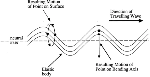
The process by which the oscillatory motion of the elastic body is transformed into motion in the moving body is illustrated in Figure 2. A point located along the bending axis of the beam will experience simple harmonic motion along a path that approximately describes a straight line normal to the axis of the beam. A point, however, located on the surface of a beam will experience an added axial component to its motion. If the shear deformation is negligibly small, the axial motion will be proportional to the lateral deflection and inversely proportional to wavelength. This side to side_motiona, combined with the displacement in the vertical direction, results in an elliptical trajectory for the surface particle. The apogee of the elliptical trajectory for a given point on the beam corresponds to the time when the crest of the lateral deflection travelling wave coincides

with that point. At any given instant, a moving body of length greater than the wavelength of the travelling wave is in contact only with those points of the elastic body which are at their apogees. The velocity imparted to the moving body by these contact points is opposite in direction to the velocity of the travelling wave.

Resulting Motion of Point on Surface Direction of Travelling Wave neutral axis

/

Elastic Point on Bending Axis

body

Figure 2- Trajectory of points on the surface and along bending axis of beam

As the motor is turned on, an object placed on top of the surface of the elastic body is subjected to a frictional force which accelerates the body to its final velocity. This final velocity is attained once the speed of the moving body matches the speed of those points on the elastic body which are at the apogee of their elliptical motion. Once these speeds are matched, the elastic body no longer exerts a force on the moving body except that needed to maintain its constant speed. The exact nature of this transient is not well understood. It is safe to assume, however, that the surface properties of the two bodies in contact will affect the performance of this type of motor. More elaborate models of this frictional force and surface interaction are beyond the scope of this thesis.

By assuming that in steady state operation the velocity of the moving body matches that of those points on the elastic body which are at the apogee of their trajectories, a mathematical expression for the velocity of the moving body as a function of the frequency and amplitude of the travelling waves can be derived using geometrical considerations. Figure 3 shows a beam of thickness T undergoing a deflection yo. The distance ý corresponds to the side motion of a point Po which gets displaced to P as a function of 0 as the wave travels through the beam.

Figure 3- Geometrical description of beam undergoing bending due to Travelling Wave

The equation describing the vertical position, y of a point on the surface of the elastic body is given by :

where:

y = y.sin(kx -

cot)

k = wave number of the travelling wave T = thickness of the beam or elastic body wo= frequency of excitation

Similarly the axial motion, C, can be described by:

T

_sin

₀

2

₍₂₎

Now for 0 << 1 (1) can be written as (3) which then differentiated by x gives us (4).

y = Yosin(kx - oot) ₍₃₎

dy

0 dx yokcos(kx - (ot) (4)

As shown by Cremer, Heckel and Ungar [7], shear deformation is negligible if the wavelength of a travelling wave is at least six times greater than the thickness of the beam. This implies that for such wavelengths, Bernouilli-Euler theory applies and

dy

dx

Thus the axial deflection of a surface particle becomes :

=T

Yokcos(kx -cot)

2 % (5)

The time derivative of (5) gives us an expression (6) which is equal to the lateral velocity of a point on the top surface of the elastic body. This equation sets an upper limit for the speed of the moving body as given by equation (7).

= velocity = o cos(kx- o t)

(6)

₍₆₎

III- Design and Construction

Design Goals

The primary goal of this project was to build an ultrasonic travelling wave motor capable of displacing an object along a straight line. The secondary goal was to maintain the motor's design as simple and practical as possible. This was essential if entertaining the possibility of finding commercial applications for the motor and for purposes of making a laboratory prototype work. The only constraints placed upon the design were the following:

* The motor had to be small and simple enough as to allow its construction with the machine tools available, and in a time frame of approximately 3 months.

* The motor had to operate in a stable fashion, without the assistance of any feedback control system.

Overall Configuration Selection

While designing the motor, three different overall configurations were evaluated, each one of them capable of producing linear motion. These configurations can be described best as: treadmill-like motors, straight beam motors, and racetrack-like motors.

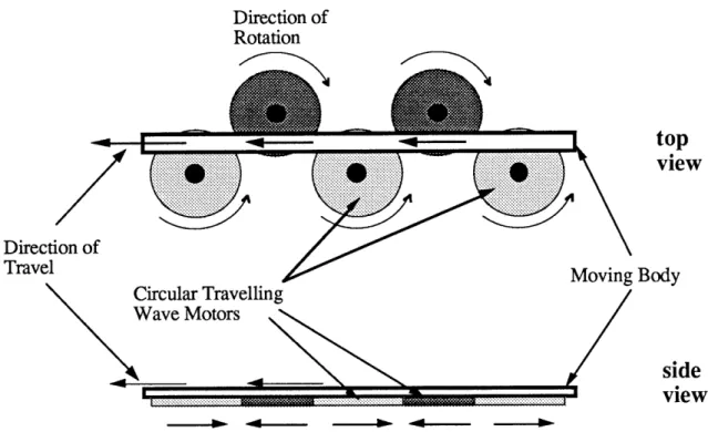
Treadmill-like Motors : This motor configuration achieves linear motion by making use of existing rotary travelling wave motors and arranging them in a fashion similar to the one depicted in Figure 4. From the figure, however, it is apparent that this

arrangement is a very inefficient way of producing rectilinear motion. Because of its inherent inefficiency, this configuration was not pursued any further

Direction of Rotation

top

'V

Direction of

Travel _{Moving Body}

Circular Travelling Wave Motors

side

view

Figure 4- Treadmill Configuration. Linear motion of a body is achieved by making it interact with parts of rotary traveling wave motors.

Racetrack-like Motors: This configuration addresses the main problem of generating travelling waves in a straight beam of finite length : the energy propagated by a travelling wave must be generated at one end and dissipated at the other. This configuration solves this problem, by avoiding it. By wrapping the track around itself the energy in the travelling wave does not have to be dissipated or created, it simply has to be re-directed around the circular portions of the track so that it can be harnessed again in the opposite straight segment of the racetrack.

This configuration avoids the problem of creating or dissipating the energy at the ends of the straight segments, by introducing the problem of creating a discontinuity in the

wave impedance of the track. This discontinuity appears at the transition from a straight to a circular section of the track, and vice versa.

Several alternatives exist to designing a motor with a racetrack configuration. Figure 5 illustrates a motor in which the travelling waves move along the outer surface of what resembles the tread of an army tank. In fact, while in operation, the motor displaces itself in a fashion similar to that of an army tank. The curve section introduces coupling between bending and extensional wave types.

Duirction

of

m'

{{t

Ground

Figure 5- In plane racetrack configuration for travelling wave motor.

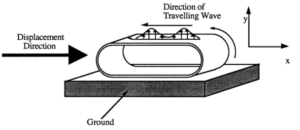
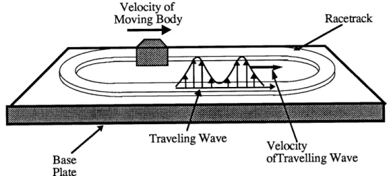
Another possible configuration is that of a flat racetrack similar to the one depicted in Figure 6. The travelling waves move along the track and allow objects placed on its surface to be displaced around the length of the track. The curved section introduces coupling between bending and torsional wave types, which might be reduced or removed by design of an asymmetric cross section.

Velocity of

Moving Body Racetrack

Traveling Wave

Base ofTravelling Wave

Plate

Figure 6- Flat track configuration. Piezo ceramics in the bottom of the track induce transverse travelling waves. Moving body travels in opposite direction of travelling wave.

Straight Beam Motors : This motor configuration fully addresses the problem of creating a travelling wave pattern in a straight beam of finite length: If the energy of a travelling wave is not totally dissipated at the end of a beam, part of it is reflected back thereby interfering with those waves that are still travelling towards the end of the beam. This will complicate the dynamics of such a motor and may affect the performance as a motor.

To solve this problem, one must attach to the ends of the beam systems that will behave as semi-infinite beams, thus artificially changing the dynamics of the finite length beam into that of an infinite medium. Kuribayashi, et al [6], implement this solution by connecting piezoceramic transducers at the ends of the beams using a specific geometric configuration and actuating the transducers so as to cancel reflections at one termination while launching waves at the other end. This is inelegant and very inefficient since most of the power injected into wave propagation is dissipated by wave absorption and does no useful mechanical work.

The configuration selected was that of a flat racetrack, since it does not require any sophisticated control system to implement it, as is the case with the straight beam configuration, nor is its construction too elaborate as is the case of the tank-tread track configuration. The flat racetrack consists of two straight beams interconnected by two semicircular beams. ( See Figure 6 ) The track is made out of a single piece of aluminum and its total length, when measured along its centerline, is equal to an integer number of wavelengths in order to increase motor performance by taking advantage of resonant effects. The bottom side of the racetrack is covered with a thin layer of piezo electric ceramics. The piezo ceramics are driven electrically so as to generate and sustain transverse travelling waves along the length of the track. Small objects, referred to in this paper as "sliders", rest on the top surface of the track and get pushed around it by virtue of the frictional effects described in section II.

Theoretical Considerations

The dynamic characteristics of the motor are entirely defined by the material properties of the racetrack, its cross sectional dimensions, and the radius of curvature of its circular segments. Therefore, the task of designing a motor that meets certain specifications is limited to selecting the appropriate values for these dimensions. This selection, however, requires a deeper understanding of the equations of motion governing the transmission of waves along the racetrack.

The race track is modelled by straight and curved beams connected together. The equations of motion for both straight and curved beams will be analyzed, as well as the behavior of the waves at the junctions of these sections. The results of this analysis will provide some insight about the size requirements for the track, its operational frequency

Equations of Motion

Straight beams: The straight portions of the motor were modelled as a one dimensional Bernouilli-Euler beam. Analysis of the equations of motion lead to dispersion relations which provide a functional relationship between the track's cross sectional properties and the frequency and wavelength of the travelling waves that can be transmitted

by the track.

Figure 7 depicts a straight beam aligned along the x axis. Transverse deflections along the z axis are denoted by w, while

3,

3

z

|r

.

-Y-

L

L

L

x

Figure 7- Axis and Variable designation for straight beam equations.

The governing differential equations for this beam are the following:

ElIw""+ pAw = 0 ₍₈₎

GJ1"- _{pJ = 0}

(9)

where: E = Modulus of elasticity of the beam

I = Bending moment of inertia about the y axis. G = Torsional stiffness of the beam

p = Density of the beam

= shorthand notation for d()/dt i.e.- derivative with respect to time.

These constants usually appear in certain groupings which have a physical interpretation. The El group defines the bending stiffness of the beam while the GJ group represents its torsional stiffness. The mass per unit length of the beam is represented by pA while pJ represents the torsional inertia of the beam.

Equation (8) describes the transverse motion of the straight portions of the track while equation (9) describes their torsional behavior. Its apparent from these equations that the transverse and torsional modes of vibration are decoupled along the straight segments of the motor.

Now by assuming a solution for the bending equation of the form:

W (xt)= woe+cot where y= c+ iK

the following dispersion relations are obtained :

pA ° 2 pA )2

=

4 El _{and Y=+4 El}

These dispersion relations show the existence of four wave patterns occurring simultaneously in the structure. These waves come in pairs which travel in opposing directions along the beam. One pair, determined by the real value of y, is usually referred to as the evanescent pair since the waves decay exponentially in space. Their influence is only felt close to the point were the originating spatial disturbance occurs. The pair determined by the imaginary value of y, is the travelling set of waves. Given that k is the wave number of the travelling pair of waves, and that :

2k=2

k and

co = 2tf

where: = wavelength of the travelling waves

f = frequency of travelling waves in Hz

the following relations can be arrived at:

f pA (10)

f 27c /El

X2 pA

2

J(11)

Given the material properties of the beam E, p ) as well as its dimensions (ie.-I, A ), f becomes a simple function of X. Equations (10,11) remain valid as long as the basic Bernouilli-Euler beam assumption applies, that is, the wavelength of the waves carried by the beam has to be much greater than the beam's thickness. If the wavelength becomes too short, shearing in the beam becomes a major factor and the Bernouilli Euler model ceases to be valid. As shown by Cremer, Heckel and Ungar [7], the wavelength of the travelling waves should be at least six times greater than the thickness of the track for the hypothesis to hold. This lower limit on the wavelength, translates into an upper limit for the frequency at which the beam can be driven.

Equation (11) shows that the operating frequency of the motor can be increased by using a stiffer material, while maintaining the wavelength and cross sectional dimensions constant. By substituting into equation (11) the expressions for the bending moment of inertia, I, and the cross sectional surface area, A, it becomes apparent that :

S(12)

h = thickness of the beam (ie. track)

Equation (12) shows that the operating frequency of the motor is proportional only to the thickness of the track and that it is independent of its width.

Curved Beams : The curved sections of the track were modelled as curved beams with a rectangular cross section. Their dynamic behavior is described by a coupled pair of differential equations which relate the transverse displacement of the beam to its rotation about its twisting axis. As the radius of curvature of the beam approaches infinity, the equations of motion describing its behavior decouple and simplify to the rectilinear model of equations (8) and (9).

Figure 8 depicts a beam with a constant radius R, a transverse displacement v, and a twisting angle of 0. The system of coordinates u,v,w is aligned such that u points at the center of curvature of the beam while w remains tangent to the path length s. v remains perpendicular to the path length s. Love [1] derived the equations of motion for a circular rod of arbitrary curvature. These equations can be adapted specifically to the circular portions of the racetrack. This derivation is given in Appendix 2.

1 0 / R

//

center of curvature

Figure 8- Axis and Variable designation for the derivation of the Equations of Motion for a Curved Beam.

The equations of motion for the curved beam are the following:

where: EIv''+ pA -1 (EI + GJ)P3 + -1GJv" R 1 EIP

GJd"- pJ =

(El

+

GJ)v"+

v = transverse displacement of a particle

P = the angle of twist about the twisting axis

' = shorthand notation for spatial derivative do/ds

R = radius of the beam

(13)

(14)

These equations state that, if the radius of curvature of a beam is finite, the out of plane motion of a transverse wave will produce torsional waves. As the radius of curvature becomes smaller, the magnitude of the coupling terms becomes larger. This implies that a smaller radius of curvature hinders the performance of the racetrack because a greater amount of energy is taken away from the transverse travelling waves in order to generate the torsional waves.

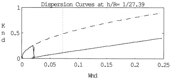
Quantifying this effect is important for design purposes. A tradeoff between the radius of the circular sections of the track and the amount of coupling between transverse and torsional modes has to be evaluated. The dispersion curves for waves travelling in a circular section of the beam offer valuable insight to this behavior. These can be obtained by translating equations (13) and (14) into state-space form and forming a transition matrix. The eigenvalues of this matrix reveal which wavetrains are evanescent (ie- real eigenvalues) and which ones are travelling waveforms (ie.- purely imaginary eigenvalues ). The dispersion curves, in this particular instance, were found to be most useful in their non-dimensional form. Hence, we proceed to non-non-dimensionalize equations (13) and (14), translate them into state-space form, and obtain the eigenvalues of the transition matrix.

The variable changes and groupings used were the following:

I = GJ + El and D = EIGJ

where I and (D are defined purely for convenience to simplify the written expressions. Then there is:

coh 2 E

nd C where: P

where ond corresponds to a non-dimensional frequency expression. In this case, Co has been non-dimensionalized by c, the velocity of longitudinal waves in the beam, and by h,

the thickness of the beam. The bending moment of inertia and hence the wavespeed is most sensitive to changes in h.

The last grouping used:

h --

R

was defined as the ratio between the thickness of the beam, h, and the radius, R. The theoretical performance of a given track design can now be evaluated as a function of the non-dimensional curvature E. In the limit, a small value of E corresponds to a track that behaves like a straight beam, with little or no coupling between the transverse and torsional modes. A big value of E will result in a large amount of coupling between the torsional and transverse modes of vibration.

Non-dimensionalization of equations (13) and (14) lead to equations (15) and (16) respectively: (h3v'"') = (G)2- 2}(hv") + pA El + El- P C2 (15) (2 WOi 2 pJco 2_C2 (h2 , E H nd 1(hv, ) ' GJ GJ

( +(h)

These equations correspond to the non-dimensional equations of motion for the curved sections of the motor. Rewriting them in state-space form, we obtain a matrix equation of the form:

dh

h- X = AX ds

where X is the state vector and A is the transition matrix. These matrices are the following: V h V' hv" 2 Vfi

h

I'

,3

El -

Wd

2

Given this A matrix, it is now possible to determine its eigenvalues and plot their imaginary component (ie- the wavenumber of the travelling waves) as a function of the non-dimensional frequency. Figure 9 illustrates both the torsional (normal line) and the transverse (dashed lines) travelling wave modes for different values of E (ie.- h/R).

As the radius of curvature of the track increases relative to its thickness, the cutoff frequency of the transverse mode decreases. This cutoff frequency corresponds to the frequency value below which, the circular beam cannot serve as a waveguide for transverse waves. Furthermore, this cutoff frequency corresponds to a wavelength which is equal to the radius of curvature of the track.

0 0 El 0 0

0

X __

0.05

0.1

0.15

0.2

0.05

0.1

0.15

0.2

Dispersion Curves at h/R= 1/50

0.05

0.15

0.25

Figure 9- Non-Dimensional Dispersion Curves for Circular Beams. 0.5 0

0.25

0.25

From a design point of view, the operating frequency of the motor is bounded on the lower side by the consideration that the wavelength of the travelling waves in the track has to be smaller than the radius of curvature of the curved sections of the track. On the other hand, the upper limit for the operating frequency of the motor is dictated by shearing effects of the beam. Since the thickness of the track remains the same in both the curved sections of the track as well as the straight ones, the upper limit of the operating frequency of the motor was chosen to be the same as that for the straight sections: the frequency has to be lower than the value that corresponds to a wavelength six times greater than the thickness of the track.

Scattering Analysis

Dispersion curves provide an estimate on how a disturbance will travel through a given section of the racetrack. The race track, however consists of four distinct sections: two straight ones and two curved ones. The junction between a straight section and a curved one can create problems because of impedance mismatch. This may cause unwanted reflections.

If the impedance between two adjacent sections is perfectly matched, a wave travelling along the first section will move onto the second section without noticing any changes on the medium its traveling on. Two perfectly bonded straight beams of similar cross sectional dimensions, would be an example of perfect impedance matching.

The dispersion relations for a straight beam and a curved beam are different, hence, there is probably an impedance mismatch at their junction. As the radius of curvature of the curved section gets smaller, this mismatch increases. Scattering analysis of the junction provides a way to quantify the effect of this impedance mismatch.

Figure 10 shows the notation convention used to designate wavetrains going into and out of a junction. Notice that each section of the track has six different wavetrains corresponding to it. Four of these wavetrains correspond to the transverse vibrational modes and represent solutions to the fourth order beam equations of motion (equations 8 and 13). The other two, correspond to torsional modes of vibration and represent solutions to the second order torsional equations of motion (equations 9 and 14).

a es unction straight beam Sbtos bes curved beam

Name Code for Wave Trains

a =

into node

b =

out of node

to = torsional wave

e =

evanescent wave

t =

travelling wave

s

= straight section

c

= curved section

Figure 10- Convention Used for Designating the Various Wavetrains Common to a Junction

As a wavetrain enters a junction, part of it gets reflected, while part of it gets transmitted through the junction. All wavetrains entering a junction are designated by a letter a, while those wavetrains leaving a junction are designated by a b. A perfect

U

transmission at a junction implies that a given wave mode entering a junction will leave it with the same amount of energy it entered. If the transmission is not ideal, the energy of an incoming wavemode will be distributed between the reflected wave modes and the transmitted ones. If there is coupling between the various modes, a scattering effect will occur at the junction by which a given wavemode will excite other wavemodes other than its own. As a result, of this scattering, it is possible for example, that an incoming transverse wave may result in both an outgoing transverse and torsional waves.

The following scattering analysis will result in a scattering matrix which relates the outgoing wave modes at a junction as a function of the incoming wavemodes. This analysis will use the the boundary conditions at the junction in their dimensional form.

At the junction between the straight beam and the curved beam, there are six boundary conditions which must be satisfied. They are the following:

vc = s --- _{> equal displacements}

S=V _{--- > equal slopes}

s = --- > equal twist angles Elsy "'= Ely"' _{--- > Shear balance}

EIPc

Ely I"= ElIv C'"

El R --- > Moment Balance

GJv '

GJds'= GJpc'+ _R -c _{--- > Torsional Balance}

where the subscript "c" refers to a variable related to the curved beam, while a subscript "s" refers to a variable related to the straight beam. (Note: w as defined in Figure 8, is equal to

vs, and

3

Ps

ElG

GJp '

the boundary conditions can be re-written in matrix form as follows :

I U U U U 0- U U U U U 0 1 0 0 0 0 0 -1 0 0 0 0 00 1000 0 0 -1 0 B 0 R 000 100 0 0 0 -1 0 0 0000 10 0 0 0 0 -1 0 - GJ O O O O1 O OR

which can be also expressed as :

[BsB _{c] =}

0

where Bs corresponds to the first 6 x 6 block and B_c corresponds to the second 6 x 6 block

matrix.

Now, using Yc and Ys as state vectors, Fourier Transformed equations (8),(9) and (13),(14) can be re-written in state space form. These corresponding matrices are the following: II I • 71 • • • 1 • •• • • f 31 Irl f31 ~ t

=s

\'Yc)

0 1 0 1 0 0

El

(El

+ GJ)

GJ

R2

where As(co) corresponds to the straight beam and Ac(C) corresponds to the circular beam. Let es be the matrix of eigenvectors of As(o) and ec be the matrix of eigenvectors of

Ac(O) . Then introduce the similarity transformations :

Ys = esWs and Yc= ecw

where ws and wc are columns of wave mode coordinates [8,9] travelling independently

along the straight and curved segments respectively. The Boundary conditions can then be written as :

[Bses i Bce

J

which can be rearranged into outgoing and incoming wave modes such that: As(o) = 0 1 0 0 0 0 Ac(O) = pA 2 - pJC02) 1 GJ 0 p

[Ba:Bb b)= ₀ B a + B b8 = 0

(17) where i and b are the incoming and outgoing wavetrain vectors defined according to the conventions in Figure 10, as follows:

Uec bts b toc bes

b

ts

bt

ats

By performing a partial inversion of equation (17), the outgoing wavetrains can be expressed in terms of the incoming ones (18). The matrix that relates them is the scattering

matrix of the junction between the straight beams and the circular beams.

-1

bF=-Bb

Ba--1 Scatter =- _{Bb Ba}

S= (Scatter)'d

Given the way in which the vectors i and 6 are defined, the scattering matrix provides information on how much of a given wave mode is reflected, and how much is (18) ' --L , I "" ,

transmitted at a junction. The scattering matrix is a 6x6 matrix which can be understood as follows: Scatter =

Transmission

Reflection

IJ

The elements along the main diagonal represent the extent to which a given wave mode transmits through the junction. Perfect transmission would imply that the scattering matrix is equal to identity. The presence of reflection at the junction and cross coupling between wave modes, produces non-zero entries in the off diagonal terms. Since the equations used for this analysis are in dimensional form, those elements along the main diagonal of the scattering matrix represent a fraction of unity in which 1 is equal to perfect transmission of that wave mode through the junction. Similarly, the elements along the diagonals of the reflection block matrices represent a fraction of unity in which 1 corresponds to total reflection of a given wavemode.

Because of their mixed units, the other elements of the scattering matrix don't provide much insight about the extent to which wavemodes are coupled, unless the columns of the matrix are non-dimensionalized so that they represent the energy delivered by each wavemode. This extra work becomes unnecessary however, if the values along the main diagonal indicate that there is good transmission at the junction.

As the radius of curvature of the curved sections of the track increases, the scattering matrix approaches the identity matrix. Conversely, as the radius of curvature of the track decreases, coupling terms appear in the off diagonal positions of the scattering

m

I

matrix while the elements along the main diagonal decrease in magnitude from their ideal value of one.

From a design point of view, transmission at the junction would be optimized if the radius of curvature of the circular portions of the motor was equal to infinity (ie.- there would be no discontinuity). In practical terms the radius of curvature of the track should be selected such that the diagonal terms of the scattering matrix approach unity within an error that may be deemed acceptable.

Cross Sectional Banking of the Track

The primary concern of both the dispersion and scattering analysis was to evaluate, the extent to which coupling between torsional and transverse modes occurred as a result of the geometrical configuration of the race track. This section, however, investigates the possibility of eliminating the coupling between bending and torsion in a curved beam by varying the cross sectional properties of the curved beam.

A simple approach to the problem consists in taking a plate viewpoint; modelling the curved segment of the track as a series of infinitesimally thin beams only capable of deflecting transversely. Furthermore, it is convenient to assume that the beams are not coupled to one another. Given this model, the problem of decoupling torsional and transverse modes in the racetrack boils down to turning the wavefront so that it follows the track. The wavefront is turned by forcing the waves travelling in the outside of the track to

go faster than the waves travelling in the inside of the track.

The speed of a travelling wave is given by equation (19):

c=X

f

₍₁₉₎

After substituting in the following expressions:

27pA bh

- k El and 12

we arrive at equation (20) which shows that the velocity of a travelling wave is proportional to the thickness of the track to the power of one half.

1

Eh

c = 2 1 2_p

(20)

Figure 11 illustrates a section of a curved beam. The centerline of the track is located at a distance r, and the wavespeed at that radial location is c. During a given length of time t, the wavefront displaces itself by a distance ds along the centerline. Waves travelling on the outside of the track, need to travel the same angular distance in the same amount of time, which means that co has to be greater than c. Conversely, ci, at the inside of the track, has

to be smaller than c.

Figure 11- Curved Section of Track. Subscript "i" refers to inner radius and the subscript "o" refers to the outer radius.

The change in speed of the waves throughout the width of the track can be accomplished by varying the thickness of the track across a given cross section. Given that the length of time t can be expressed as :

ds _i dso _ds

C. _. C _o C

(21)

Clearly the thickness should vary quadratically with the radial distance from the center of curvature. This is difficult to machine, and we rather consider a thickness distribution linear with radial distance.:

h ( 4 r2- _{4rb + b}2 )

i _{4 r}2

h ref ₍₂₂₎

h ·=(4r2+ 4rb+ b 2

0 4r2 href ₍₂₃₎

where: hi = thickness of the beam at a distance r-b from the center of curvature

ho = thickness of the beam at a distance r+b from the center of curvature

r = radius measured along the centerline of the track.

href = thickness of reference beam with plain rectangular cross section

Now, by substituting equations (22) and (23) into equation (24), which assumes that the thickness of the track varies in a linear fashion:

h. + h

h _avg = ₂

(24)

we arrive at equation (25):

havg = average thickness of the track with variable cross section

This relationship implies that if the thickness of the track is varied linearly, the wavefront will follow the shape of the track as long as the ratio of the width to the radius of curvature of the track is small. If this ratio is not small, the linear approximation cannot be used and the thickness of the track would have to vary quadratically. From a construction point of view, varying of the cross sectional thickness of the track in a linear fashion would be easier than varying it quadratically. For example, a curved beam with a rectangular cross section, with a radius of 2.5 inches, a width of half an inch and a thickness of 80 milli-inches along its centerline would have to be altered so that the thickness along the inside of the track was 51 inches thick and the thickness along the outer radius became 97 milli-inches.

An alternative to varying the cross sectional thickness of the track is to vary its mass distribution. Rewriting equation (20) as a function of t, the mass per unit length of the beam, we obtain :

c= 2•Erco

(26)

which implies that the velocity of the traveling wave is inversely proportional to the fourth root of g. After performing an analysis similar to to the one performed for the cross sectional variation of thickness, we obtain the required values of gt, for the outer and inner sections of the track in terms of the gt along the centerline of the track.

4

r

2 (28)

where: pto = mass per unit length along the outside of the track. ti = mass per unit length along the inside of the track. g = mass per unit length along the centerline of the track

Varying the density across the width of the track is in practice not feasible. Shifting the center of mass of the beam by placing a lumped portion of mass of higher density on the inside of the track, such that the resulting center of mass is similar to that achieved by a functional variation of density, is feasible. Figure 12 indicates the position of the center of mass of a rectangular beam with a constant density and the center of mass of a rectangular beam whose density varies linearly between the values defined by equations (27) and (28). Using a beam with similar dimensions as that of the previous example, we obtain through equations (27) and (28), that the inside of the track has to have a density 1.5 times greater than the density of the beam with a rectangular cross section. Similarly the outside of the track has to have its density value decreased by a factor of 1.46 relative to the density of the beam with a rectangular cross section.

.

L. ... ..

i, II i

x=b x=0 shift shift

Simple Beam Variable Added Lump

Density

Figure 12- Side Shift of the Position of the Center of Mass across the Width of the Beam due to Variational Distribution of p. and due to Addition of Lumped Mass to One Side. (The center of Curvature is located to the Right hand Side of the Cross sections.)

The center of mass of a rectangular beam is located along the middle of the beam. If we assume that the the mass per unit length varies across the width of the track as shown in Figure 12, then g can be written as a linear function :

g = cx + d (29)

where, for the example given, c = .1596 and d= -.1734.

The shift of the position of the center of mass in a beam with a density distribution described in equation (29) is equal to:

shift = b

2

3( 0)

where: b = width of the track.

For the example at hand, a beam with a linearly varying gt, would have a center of mass located 25 milli-inches away from the center of mass of a beam whose gt remained constant. The direction of this shift is towards the center of curvature of the track.

A similar shift of the center of mass can be attained by adding a lumped mass, of greater density than the rest of the track, to the inner radius of the curved beam. See Figure 12. The relative shift of the center of mass for this configuration is given by equation (31):

shift =

(1)

where: x = width of the cross section of the lumped mass gI1 = mass per unit length of track

By using this approach, the 25 milli-inch shift of the center of mass from the previous example can be duplicated by adding a 13 milli-inch thick strip of lead to the inside of the aluminum track.

Another approach of analyzing the torsion bending coupling along the curved sections of the track with offset between the elastic axis and section center of mass, is to add another term to the governing equations of motion, (13) and (14). It may be possible that they decouple at the desired operating frequency of the motor. As shown by Bisplinghoff [10], this additional term takes into account the separation between the center of mass of the beam and its elastic axis. By incorporating this term to equations (13) and

(14), we obtain the following:

EIv""+ pAA= -(El + GJ)y"+

S,+

R (32)

S1 EIP

GJ"- pJ =- R((El + GJ)v"- S +

RR (33)

where Sy = _{pAe and e is defined as the separation between the center of mass and} the elastic axis.

In order to decouple equations (32) and (33), the terms in 0 of equation (32) as well as the terms in v of equation (33) have to vanish. This can be accomplished by setting:

(El + GJ)

e=2

p ARf 2 ₍₃₄₎

By selecting an operating frequency of 27230 Hz and using the cross sectional properties corresponding to the beam of the previous example, we obtain a value of e equal to 31.7 mill-inches. This value is approximately 20 % larger than the value of the center of

mass shifts obtained using the simplified beam models. This suggests that these simplified beam models are relatively good and that the torsional extensional coupling along the curved sections of the beam can be greatly reduced by simply placing a strip of lead along the inside of these sections.

Piezo Ceramic Layout

In order to induce travelling waves along the racetrack, piezo electric ceramics are glued to the bottom side of the track and excited so that they produce a moving wavetrain. The disposition of the ceramics on the track is not unique. An approach commonly used in the travelling wave motors developed by the Matsushita Research group [11,12] is to generate a travelling wave by actually producing two standing waves and carefully phasing them so that their resultant is travelling. This approach requires a symmetric disposition of the piezo ceramics. Usually one side of the track is in charge of driving one of the standing waves, while another set of piezos mounted on the opposite side of the track, drive the second standing wave. The phasing between both sets of piezos is accomplished by allowing a physical separation between both sets of piezos equivalent to a quarter of the wavelength of the travelling wave. See Figure 13.

Another way of implementing two standing waves is to collocate the piezos responsible for driving the different standing waves by mounting them one on top of the other. The phasing between the standing waves is once again accomplished by physically displacing one set of piezos by a quarter wavelength relative to the other. This configuration, however, is impractical, since access to the lower layer of ceramics is restricted once the top layer is mounted. Collocation can also be achieved by setting the two banks of piezos side by side along the width of the track.

Piezo Standing Wave A

Ceramics

SI

+

1/2 X _{Standing Wave B}

II

Resulting Travelling Wave

Figure 13- Piezo Layout Configuration which Drives Two Standing Waves Phased Which Results in a Travelling Wave. Piezo ceramics labeled with an A drive one of the Standing waves, while those ceramics labeled with a B drive the other standing wave.

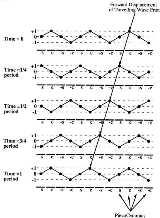
A simpler way of driving the travelling waves along the motor is to cover the whole bottom side of the track with piezo ceramics and to drive them in a sequential manner to generate a rippling effect which thereby produces the travelling wave. The piezo ceramic segments are a quarter wavelength in length and have the same width of the track. Each segment is driven by a different electrical signal : a sine, a cosine, a negative sine, and a negative cosine wave respectively. The electric signals are exactly in phase relative to each other. This pattern is repeated throughout the length of the track an integer amount of times such that there is an integer amount of wavelengths being generated by the track. Figure 14 illustrates schematically a portion of the track being excited by piezo ceramics. The letter under the ceramics indicates which electrical signal is driving that portion of the track. An s corresponds to a sine wave, a c to a cosine wave, a -s to a negative sine wave and a -c to a Uncovereo

negative cosine wave. Figure 13 also illustrates how the superposition of these four signals leads to a rippling effect which corresponds to a travelling wave moving along the length of the track.

Forward Displacement of Travelling Wave Front

Time1/

+1---

---s c ---s -C ---s c ---s -c S C ---s -c

+1--- ---

---

+1

-

-- -

-- --

-- -

-- - ---

-Time =1

0

- --- --- --- --- ---

-period

-1

-- -- -- - - -- -- -- -- -- -- -

Figure _{14- Schematic Representation of a Portion of the Track Undergoing Excitement by} Piezo Ceramics. In One Full Cycle, the Wave Pattern Displaces Itself by One Wavelength.

This last piezo ceramic configuration was chosen since accurate alignment between the piezos and the track is not required. Furthermore, this configuration also permits the even distribution of piezos throughout the whole surface of the track. This eliminates the problem of having cross sectional discontinuities along the track such as portions of the track being made of aluminum and ceramics while other portions of the track are made entirely of aluminum. Discontinuities along the track are to be avoided since they represent junctions at which wavetrains can undergo scattering.

As the operating frequency of the motor is increased the length of the wavelength in the track decreases. Since this ceramic layout configuration requires four piezo etchings per wavelength and since there is a practical limit to the size of piezos that can be etched using available technology, there is therefore a practical limitation to the operating frequency of the motor. From a design perspective, the operating frequency of the motor has to be selected such that the wavelength of the waves is at least six times the thickness of the track as well as large enough to allow four piezo segments to be accurately etched.

Corrections due to Piezo Layer

The dynamic analysis of the various segments of the track has neglected to take into account the presence of the piezoelectric ceramics attached to the track as well as the glue layer bonding them together. In order to model more accurately the dynamic behavior of the racetrack, the track's overall stiffness, torsional rigidity and mass per unit length values were adjusted to take into account the presence of the piezo ceramics. The ceramics were thin, not more than 10% of the total thickness of the aluminum track. The effects of the glue layer between the aluminum track and the ceramics was neglected.

Given the material properties of the G1195 piezo ceramics used ( see Appendix 5 ), the mass per unit length of the composite (ie- aluminum and piezo) race track was evaluated using an area weighted average of its mass densities as follows:

pA= Pabh+ ppbhp ₍₃₅₎

where: pA = mass per unit length of the composite track

Pa = density of aluminum

pp = density of G1195 piezo ceramics h = thickness of the aluminum track hp = thickness of the piezo ceramic layer

b = width of both the track and the piezo ceramic layer

Similarly, the overall moment of inertia, I, of the composite beam was reevaluated about the composite centroidal axis using a modulus weighted formula. The shift in the centroidal bending axis due to the presence of the piezo ceramic layer was estimated as follows:

(rh

p

₊

_2hhp+h

Z1 _{2(h + h r)}

(36)

where : zcl = shift of the centroidal bending axis

r = _{ratio of the modulus of elasticity of aluminum and the piezo ceramic} such as defined by :

E.

piezo

r= m

The bending moment of inertia of the composite beam about the N centroidal axis was then evaluated by:

3 2

I= _{+ b.z -} (h, + )2 + +rbh - ₍₃₇₎

where : I = bending moment of inertia of composite track

The racetrack's polar moment of inertia was estimated by assuming that the ratio of the modulus of elasticity between the composite beam and the aluminum beam was the same as the ratio of their torsional stiffness. Hence the value for the polar moment of inertia of the composite track was approximated by using the following expression:

(38)

where: J = polar moment of inertia of composite beam J = polar moment of inertia of aluminum beam

The modified values of E, I, and J as derived in this section were used in all calculations including the ones from preceding sections.

Design Iteration Procedure

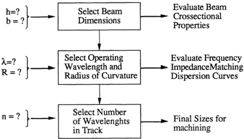
Given the overall configuration of the motor and having selected Aluminum as the material for its construction, the remainder of the design process consisted in selecting the dimensions of the track and evaluating its performance according to the models developed in the previous section. These last steps were performed in an iterative fashion until a motor design feasible to be constructed at our labs was arrived at. Figure 15 shows a block diagram of the steps involved in the design iteration process.

h=? ]Select Beam Evaluate Beam h=?1- .SCrossectional

b = ? Dimensions Properties

X=? Select Operating Evaluate Frequency

R = ? _ Wavelength and ImpedanceMatching Radius of Curvature Dispersion Curves

=? Select Number

n = ? of Wavelenghts Final Sizes for

in Track machining

Figure 15- Block Diagram of Design Iteration Process

The first step involves choosing the cross sectional dimensions of the track. Once h and b are selected, all other relevant cross sectional properties of the track can be evaluated. Further analysis then demands that the cross sectional properties of the track be adjusted to take into account the influence of the piezo ceramics glued on the bottom side of the track. Having obtained estimates on the bending and torsional stiffness of the composite track it is necessary to predict the maximum static deflection that can be achieved by a beam of the prescribed dimensions. If the thickness of the piezo ceramics relative to the aluminum track is too small, the piezos may not have the authority to command the necessary deflection needed to attain a given operational speed. Since the dynamic amplification obtained by operating the track at resonance is unknown, the static deflection alone should be capable of attaining the selected operational speed of the motor. Hence, once in operation, the true speed attained by the motor will be greater than the design speed. Appendix 7 contains a description of the model used to describe the forces on the track due to the piezo actuators and shows the procedure used to estimate its static deflection.