An adaptive framework for high-order, mixed-element numerical simulations

An adaptive framework for high-order,

mixed-element numerical simulations

by

by M~sOF TECHNOLOGYE

Philip Claude Delhaye Caplan

JUN

162014

B.Eng., McGill University (2012)

Submitted to the Department of Aeronautics and Astronautics

in partial fulfillment of the requirements for the degree of

Master of Science in Aeronautics and Astronautics

at the

MASSACHUSETTS INSTITUTE OF TECHNOLOGY

June 2014

©

Massachusetts Institute of Technology 2014. All rights reserved.

Signature redacted

A uthor .... ...

D~partment of Aeronautics and Astronautics

May 22, 2014

Signature redacted

C ertified by .

...

David L. Darmofal

Professor of Aeronautics and Astronautics

Thesis Supervisor

Signature redacted

A ccepted by .... ...

Paulo C. Lozano

Associate Professor of Aeronautics and Astronautics

Chair, Graduate Program Committee

An adaptive framework for high-order, mixed-element

numerical simulations

by

Philip Claude Delhaye Caplan

Submitted to the Department of Aeronautics and Astronautics on May 22, 2014, in partial fulfillment of the

requirements for the degree of

Master of Science in Aeronautics and Astronautics

Abstract

This work builds upon an adaptive simulation framework to allow for mixed-element meshes in two dimensions. Contributions are focused in the area of mesh generation which employs the L' norm to produce various mesh types. Mixed-element meshes are obtained by first using the L' norm to create a right-triangulation which is then combined to form quadrilaterals through a graph-matching approach. The resulting straight-sided mesh is then curved using a nonlinear elasticity analogy. Since the element sizes and orientations are prescribed to the mesh generator through a field of Riemannian metric tensors, the adaptation algorithm used to compute this field is also discussed.

The algorithm is first tested through the L2 error control of isotropic and anisotropic

problems and shows that optimal mesh gradings can be obtained. Problems drawn from aerodynamics are then used to demonstrate the ability of the algorithm in prac-tical applications. With mixed element meshes, the adaptation algorithm works well in practice, however, improvements can be made in the cost and error models. In fact, using the L -generated meshes inherits the same properties of traditional trian-gulations while adding structure to the mesh. The use of the L -norm in generating tetrahedral meshes is worth pursuing in the future.

Thesis Supervisor: David L. Darmofal

Acknowledgments

My experiences at MIT taught me more about life than they did about equations. I

need to thank everyone who was involved in making my time here so memorable.

I start with my team of advisors, who pushed me when I needed to be pushed but whose knowledge, insight and humour kept me motivated over the past two years. Prof. David Darmofal, thank you for supporting me in exploring a wide range of topics and for encouraging me to always dig further. Dr. Steven Allmaras, your humble knowledge of all things CFD contributed to such a vast learning experience. Marshall, your coding practices leave me well-prepared for my ncxt chapter (yes, I'll write unit tests). Bob, your honest opinion of my work was always appreciated; thank you for being available over the past few years and I will miss working with you.

I must also acknowledge the influence of my undergraduate professors at McGill

University for shaping me into the engineer I am today: Prof. Charles Roth for giving me the opportunity to teach at an undergraduate level and Prof. John Lee for instill-ing a deep understandinstill-ing of the fundamentals. I am eternally grateful to my mentor, Prof. Siva Nadarajah, for introducing me to reasearch in CFD and for leaving me well-prepared for the challenges at MIT.

In September 2012, Steven, Jun and I were thrown into 31-213 and I could not have been luckier to have shared so many laughs with you guys; you really made this experience worthwhile. Huafei, thanks for being so patient while getting us started with ProjectX. Carlee, Jeff, Savithru and Yixuan, thank you for restoring a fun at-moshpere in our office as we all complained about writing our theses. Gracias a los

espafioles para colonizar edificio 31: David, Ferran, Joel - this of course also includes

Hemant, Abby and Dr. Nguyen. I will miss hearing the mix of Spanish and Catalan shouts as a fntbol match plays in the background. In particular, I thank Xevi for sharing his expertise in meshing, geometry and C++; your encouraging words kept

me on track i prometo que aprendr6 Haskell a l'estiu. I'd also like to thank Eric Dow for making sure all the computational resources in the ACDL were functioning smoothly and for teaching me the ways of system administration. Thank you to the second half of the ACDL: Patrick, Alessio, Chaitanya, Remi, Giulia, Marc and Xun for getting everyone out of the lab to relax.

I thank all my roommates and neighbours for putting up with my drumming and

to my friends for making my time outside the lab so enjoyable: Fernando, Michael, Rafa, Sami, Paul, Kavitha, Luis, Irene, Tim, Melanie and Xavier.

Maman, your hourly messages made me feel as if I were back home in Montreal and I could not have completed this work without your unconditional love and sup-port. Dad, you've been a source of inspiration in my pursuit of engineering studies and a role model and I thank you for always being there to support me. Je remercie aussi Grandmaman, Grandpapa and Nani for your endless encouragement throughout my studies.

This thesis is dedicated to my two favourite people with whom I can share any-thing. Despite 500 km between us, I love how our Skype calls are reminiscent of the times when we were 4, 7 and 9 years old. Thank you to my two brothers and best

friends, Ryan and Alex.

Finally, I would like to acknowledge financial support from the Natural Sciences

and Engineering Research Council of Canada, the NASA Cooperative Agreement

(#

Contents

1 Introduction

1.1 M otivation. . . . .

1.2 O utline. . . . .

1.3 Background ... ...

1.3.1 Error estimation and adaptation . . . .

1.3.2 Mesh generation . . . .

2 Discretization, error estimation and adaptation

2.1 Numerical discretization . . . .

2.2 Output error estimation . . . .

2.3 Metric construction . . . .

2.3.1 Mesh-metric duality . . . .

2.3.2 Mesh optimization via error sampling and synthesis

3 Mesh generation

3.1 Fundamentals . . . .

3.1.1 Geometry representation . . . .

3.1.2 Metric field evaluation . . . . .

3.1.3 Right triangle mesh generation

3.2 Surface mesh generation . . . . 3.3 Volume mesh generation . . . .

3.4 Curvilinear mesh generation . . . .

3.5 Exam ples . . . . 15 . . . . 15 . . . . 21 ... . 22 . . . . 22 . . . . 22 27 27 28 30 30 33 37 . . . . 37 . . . . 38 . . . . 38 . . . . 39 . . . . 4 1 . . . . 4 2 . . . . 44 . . . . 46

4 Numerical results

4.1 L2 error control . . . .

4.1.1 r'-type corner singularity . . . .

4.1.2 2d boundary layer . . . .

4.2 Compressible Navier-Stokes equations . . . .

4.2.1 Euler equations . . . .

4.2.2 Reynolds-averaged Navier-Stokes equations

4.2.3 Zero pressure gradient turbulent flat plate

4.2.4 Turbulent transonic RAE2822 airfoil . . . .

5 Conclusions

5.1 Sum m ary . . . .

5.2 Future work . . . .

5.2.1 Improving the local error model . . . .

5.2.2 Extension of the mesh generation algorithm to

5.2.3 Mesh curving . . . .

5.2.4 Alternative discretisations . . . .

5.3 Concluding remarks . . . .

higher dimensions

A Improving the local error model

A. 1 Error modeling techniques . .

A.2 Error model rates . . . .

A.3 Application to L2error control . .

B Connectivity tables for the embedded discontinuous Galerkin method 97 51 . . . . 51 . . . . 52 . . . . 54 . . . . 59 . . . . 59 . . . . 69 . . . . 71 . . . . 77 83 83 85 85 85 86 87 87 89 . . . . 8 9 . . . . 9 0 . . . . 9 3

List of Figures

1-1 Memory footprint of d-simplices versus d-cubes for DG, HDG and EDG

discretisations; a factor of 1 indicates both shapes incur the same

mem-ory cost . . . . 19

1-2 Memory footprint of equilateral tetrahedra versus right tetrahedra for DG, HDG and EDG discretisations . . . . 19

1-3 Reference shapes in two dimensions . . . . 20

1-4 Adaptive simulation framework . . . . 21

1-5 Initial and adapted mesh obtained using the quadrilateral subdivision technique, reproduced with permission from Marco Ceze and Krzysztof J. Fidkow ski [10] . . . . 23

2-1 M esh-m etric duality . . . . 31

2-2 Triangle split configurations . . . . 34

2-3 Quadrilateral split configurations . . . . 34

3-1 Mesh generation algorithm . . . . 37

3-2 Interpretation of a right triangle with respect to a unit Lk ball . . . . 39

3-3 Graph-matching approach . . . . 40

3-4 Curve metric description with true geometry . . . . 41

3-5 Force used to elongate or compress mesh edges according to their length under a m etric field . . . . 44

3-6 Primitive mesh operations . . . . 45

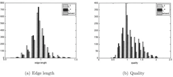
3-7 Edge length and element quality distributions for the cylinder example with an analytic metric field . . . . 48

3-8 Edge length and element quality distributions for the three-element

MDA airfoil example with a discrete metric field . . . . 48

3-9 Meshes generated by analytic (cylinder) and discrete (three-element

MDA airfoil) metric fields using equilateral (L'), right (L') and

mixed-element mesh generation techniques . . . . 49

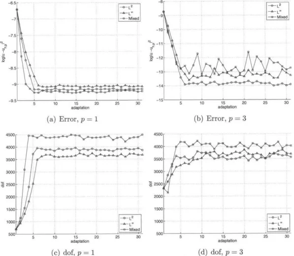
4-1 Error and degrees of freedom convergence for the corner singularity

problem . . . . 55

4-2 p = 1, dof = 4,000 optimized for the corner singularity problem, k* = 0.44 56

4-3 p = 3, dof = 4,000 optimized for the corner singularity problem, k* = 0.67 57

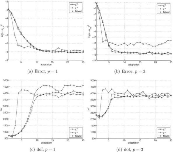
4-4 Error and degrees of freedom convergence for the 2d boundary layer

problem. The refinement factor for triangulations is set to r = 2

whereas it is set to r = 4 for mixed-element meshes. . . . . 60

4-5 p = 3, dof = 4,000 optimized mixed element meshe along with

corre-sponding size and aspect ratio distributions for the 2d boundary layer

problem with a refinement factor of r = 2, k* = 22.5, k*, = -25 . . . 60

4-6 p = 1, dof = _{4,000 optimized meshes along with corresponding size and}

aspect ratio distributions for the 2d boundary layer problem, k*1

-41.7, k*r = -50. The refinement factor for triangulations is set to

r = 2 whereas it is set to r = 4 for mixed-element meshes. . . . . 61

4-7 p = 3, dof = 4,000 optimized meshes along with corresponding size and

aspect ratio distributions for the 2d boundary layer problem, k*1 =

22.5, k*, -25. The refinement factor for triangulations is set to

r = 2 whereas it is set to r = 4 for mixed-element meshes. . . . . 62

4-8 Supersonic wedge problem setup . . . . 63

4-9 p = 1, 30,000 degree-of-freedom optimized meshes for the supersonic

w edge case . . . . 65

4-10 p = 3, 30,000 degree-of-freedom optimized meshes for the supersonic

4-11 Mach number, total pressure and total temperature distributions across

a horizontal line at y = 0.4 for the supersonic wedge case for all mesh

types with p = 1 and p = 3 discretisations . . . . 67

4-12 Artificial viscosity added near shocks for the p = 3 solution to the

supersonic wedge case with L2, L' and mixed-element meshes . . . . 68

4-13 Convergence rates for p = 1 and p = 3 adaptations for the supersonic

wedge case with L2, L' and mixed-element meshes . . . . 68

4-14 p = 1, 20k dof-optimized mixed-element mesh for the zero pressure

gradient flat plate case . . . . 73

4-15 p = 1, 20k dof-optimized triangulations for the zero pressure gradient

flat plate case . . . . 74

4-16 p = 2, 20k dof-optimized mixed-element mesh for the zero pressure

gradient flat plate case . . . . 75

4-17 p = 2, 20k dof-optimized triangulations for the zero pressure gradient

flat plate case . . . . 76

4-18 Convergence rates for p = 1 and p = 2 adaptations for the zero pressure

gradient flat plate case with all element types . . . . 76

4-19 Adapted meshes for the turbulent, transonic RAE2822 case at p = 1

and p = 2 solution orders . . . . 80

4-20 Recombined L" meshes for the turbulent, transonic RAE2822 case at

p = 1 and p = 2 solution orders . . . . 81

4-21 Mach number and mass adjoint for the turbulent, transonic RAE2822

case . ... ... 81

4-22 Drag error estimate and degree-of-freedom convergence for the

turbu-lent, transonic RAE2822 case . . . . 82

5-1 Ideal tetrahedron and triangular-based prism suitable for

recombina-tion into hexahedra . . . . 86

5-2 Mapping between ideal, master and physical elements for a q = 3

5-3 Mesh of Ursa generated by converting a grayscale image to an isotropic

metric tensor field within a rectangular domain . . . . 88

A-1 Id split configuration . . . . 90

A-2 Effective exponent in error model of Eq. (A.3) obtained using both

error modeling technqiues . . . . 93

A-3 Errors and rates obtained with both models on a coarse mesh, p = 3,

n=4... ... .... 95

A-4 Errors and rates obtained with both models on a fine mesh, p = 3,

List of Tables

1.1 dof and nnz expressions for each Galerkin method . . . . 16

1.2 Local connectivity tables for different element types, lij . . . . 17

1.3 Coupling factors for nnz calculation . . . . 18

3.1 Number of triangles (t) and quads (q) for the mesh generation examples 47

4.1 Mesh size correlation rates away from the origin for the L2 error control

applied to the corner singularity problem . . . . 54

4.2 Mesh size and aspect ratio correlation rates away from the wall for the

L2 error control applied to the 2d boundary layer problem . . . . 59

4.3 Properties of the 30,000 degree-of-freedom adapted meshes for the

su-personic wedge case . . . . 64

4.4 Properties of the adapted meshes for the turbulent, transonic RAE2822

case, p = 1. L -R stands for L -Recombined. . . . . 79

4.5 Properties of the adapted meshes for the turbulent, transonic RAE2822

case, p = 2. L -R stands for L -Recombined. . . . . 79

B.1 Connectivity factor, cij, for triangles using the EDG method . . . . . 98

B.2 Connectivity factor, cij, for quadrilaterals using the EDG method . . 98

B.3 Connectivity factor, cij, for tetrahedra using the EDG method . . . . 98 B.4 Connectivity factor, ci,, for hexahedra using the EDG method . . . . 98

Chapter 1

Introduction

1.1

Motivation

The numerical wind tunnel is widely accepted as an invaluable design tool for en-gineers. The ability to simulate physical phenomena around complex geometries at a lower cost and time investment than experimental methods facilitates the design of next-generation aircraft. The reliability of computational methods has, however,

been an active research area for the last few decades

[54].

Interest in unstructured high-order methods has given rise to some general ap-proaches for accurately simulating the physics around complex geometries at lower computational costs than existing second-order methods. In the realm of finite-element methods, these techniques branch into continuous (CG), discontinuous (DG) or hybridized (HDG, EDG) Galerkin discretisations which vary based on the nature of the function spaces housing the numerical solution as well as the number of un-knowns in the resulting system of equations.

Obtaining accurate numerical solutions under available computational resources

is facilitated by an adaptive solution process, in which either the mesh size (h) or

polynomial space of the solution (p) are refined (coarsened) to concentrate degrees of freedom near solution features. In general, these features are not known a priori and

Table 1.1: dof and nnz expressions for

error estimation techniques can be employed to localize errors in the current discreti-sation. In addition, element shape plays an important role in an adaptive solution process. For example, quadrilateral elements can provide better alignment with local solution features than triangular elements. This work aims at investigating the use of mixed-elements in a mesh-adaptative solution process.

The memory consumption of the DG, HDG and EDG schemes with d-simplices or d-cubes is first considered. Note the analysis for the EDG method is equivalent to that of the continuous Galerkin method with static condensation. The mesh is assumed to be very large such that the number of boundary faces is negligible compared to the number of elements. Without loss of generality, a single conservation law is used in the analysis. The degrees of freedom (ndof) and number of non-zero entries in the Jacobian of the governing equations (nnz) are counted:

number of degrees of freedom number of non-zero Jacobian entries

ndof , nnz

number of elements number of elements

The objective of this analysis is to compare the cost of performing a finite-element

simulation within some domain Q c Rd tessellated by meshes composed of either

d-simplices or d-cubes. The degrees of freedom can be calculated using the expressions in Table 1.1, where the quantities ndofi represent the degrees of freedom of an i-dimensional entity, which varies based on element shape. The superscript "' indicates only internal degrees of freedom are counted. For example, an i-dimensional cube has

ndofi = (p + 1)i and ndofin = (p - 1)i. The weights, gij, represent the global number of i-dimensional elements relative to the number of elements in the entire

DG HDG EDG

d-1

ndof ndof d gd-1,dndofd-1

Z

i=O

d-1

nnz c ndof d C gd_1,dndof d_1

Z

i=O

Table 1.2: Local connectivity tables for different element types, lij

Element Tri Quad Tet Hex

dim 0 1 2 0 1 2 0 1 2 3 0 1 2 3 0 1 6 6 1 4 4 1 12 20 20 1 6 12 8 1 2 1 2 2 1 2 2 1 36/7 36/7 2 1 4 4 2 3 3 1 4 4 1 3 3 1 2 4 4 1 2 -3 --- 4 6 4 1 8 12 6 1

mesh (d-dimensional entities). These are computed from

l ,i gi,d =

Ii,d

where li,d represents the local number of d-dimensional entities connected to an

i-dimensional one. A simple example consists of computing g1,2 for a triangulation,

which gives the number of edges in a mesh relative to the number of triangles; g1,2 =

3/2 since there are three edges per triangle and two triangles per edge. The assumed

connectivity tables for the current work are given in Table 1.2, which differ from those presented in [26] since equilateral simplices are assumed here whereas Huerta et al. assume structured (right-angled) simplices. More specifically, the ball around a three-dimensional mesh vertex is assumed to be an icosahedron instead of a cube. The connectivity of equilateral and right-angled triangles used here is identical to that in [26]. Similarly, the number of non-zero entries in the Jacobian can be computed by summing the weighted contributions of each d-dimensional entity as given in Table

1.1, where the coupling factor, ci represents the connectivity of an i-dimensional

entity with other entities; this factor reduces to a single value, c, for the DG and

HDG methods. For each method, the coupling factor is given in Table 1.3. Note the cij connectivity entries for the EDG method are used unchanged from [26] and are

provided using the current notation in Appendix B.

Under the assumption of unit-length equilateral simplices and unit-length cubes in some reference space, the reduction in the number of cubes versus simplices required

Table 1.3: Coupling factors for nnz calculation

Method Coupling factor

DG c = (ld,d-1 + 1)ndof d

HDG c = (ld-1,dldd_1 - 1)

d

EDG ci = T ci,jndof'nt

j=0

to fill Q is determined by the volume ratio of unit d-cubes to d-simplices:

ncubes d -1

nsimplices d! 1. ₍₁

The memory footprint of the above discretisations have been derived by modifying the work of Huerta et al. [26] to account for equilateral simplicial meshes. Addi-tionally accounting for the above volume correction, the memory footprint ratios of

d-simplices to d-cubes are shown in Fig. 1-1.

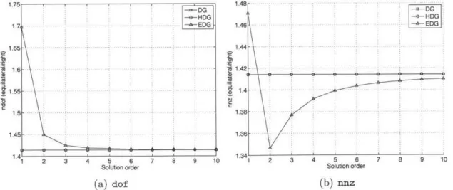
Figs. 1-1(a) & (c) show that 2-, 3-cubes consume less memory when storing solu-tion variables, regardless of the discretisasolu-tion method or solusolu-tion order. The memory needed to store the Jacobian matrix is, in general, the primary memory consumer of an implicit solver. As shown in Fig. 1-1(b), in two dimensions, the ratio of memory consumed by the HDG method with triangles versus quadrilaterals is unaffected by the solution order. In addition, a p = 1 discretisation with the DG method is more costly with triangles but immediately becomes more costly with quadrilaterals for

p > 1. On the other hand, an EDG discretisation with quadrilaterals is advantageous

for p > 1. In three dimensions, the HDG method is always less costly with hexahe-dra than with tetrahehexahe-dra. Similar to the case in two dimensions, hexahehexahe-dra are less

costly for a p = 1 DG discretisation but tetrahedra are more advantageous with this

scheme for p > 1. Also observe the EDG discretisation is always less costly when us-ing tetrahedra. Of course, these figures merely demonstrate the difference in memory consumption. Adding structure to a mesh, thereby increasing solver robustness, may trump the higher memory cost of cubes over simplices.

4-3 1 2 3 4-5.6 7 8 9 1. 11 Solution order (a) dof (d 2) 1.3 1.2 1.1 0.8 0.7 0.6 0 -- DG-- - - -- -HDG -EDG --. _- -. -.-.-.-.-.- ...- ... . 4 5 6 7 8 9 1J0 Solution order (b) nnz (d 2) -e- H-G -EDG 3 4 5- 6 7- 8 9 1 3 4 5 6 7 8 9 10 Solution order (c) dof (d = 3) 2.2 1.8 1.6 1.4 1.2 0.9 0.6 0.4 0.2 -e- DG -e- HDG A-EDG - 2- - -3 4 5--2 3 4 5 6 Solution order (d) nnz (d = 3)

Figure 1-1: Memory footprint of d-simplices versus d-cubes for DG, HDG and EDG discretisations; a factor of 1 indicates both shapes incur the same memory cost

75 -e- HDG 1.7 ---65 - -.-.--1.6 -55 - -.--.-1 .5 - - - - - - -- - .-.- . --. *-. 45-1.4 1 2 3 4 5 Solution order (a) dof 1.48 1.46 1.44 1.42 1.4 1.381-1.36

r..

Figure 1-2: Memory footprint of equilateral tetrahedra versus right tetrahedra for

DG, HDG and EDG discretisations

1. 1. 1. 1. 1 .5 4 3.5-4) 3 2.5 2 1.5 1 2 7 8 9 10 1. 1. 1! 1. 1 -e- DG -- HDG SEDG 7 10 1. 1. '0. 9 1. 4 -1 1. 7 8 9 10

1 A 14 1i1 0.9 0.9 0.9-0.8 0.8 0.8-0.7 0.7 0.7-0.6 0.6 0.6 0.5 g r 0.5 0.5 0.4 0.4 0.4 0.3 0.3 0.3 0.2- 0.2- 0.2-0.1 - 0.1 0.1-.5 0 0.5 T 0.2 0.4 0.6 0.8 1 0 0.2 0.4 0.6 0.8

(a) Equilateral triangle (b) Right triangle (c) Quadrilateral

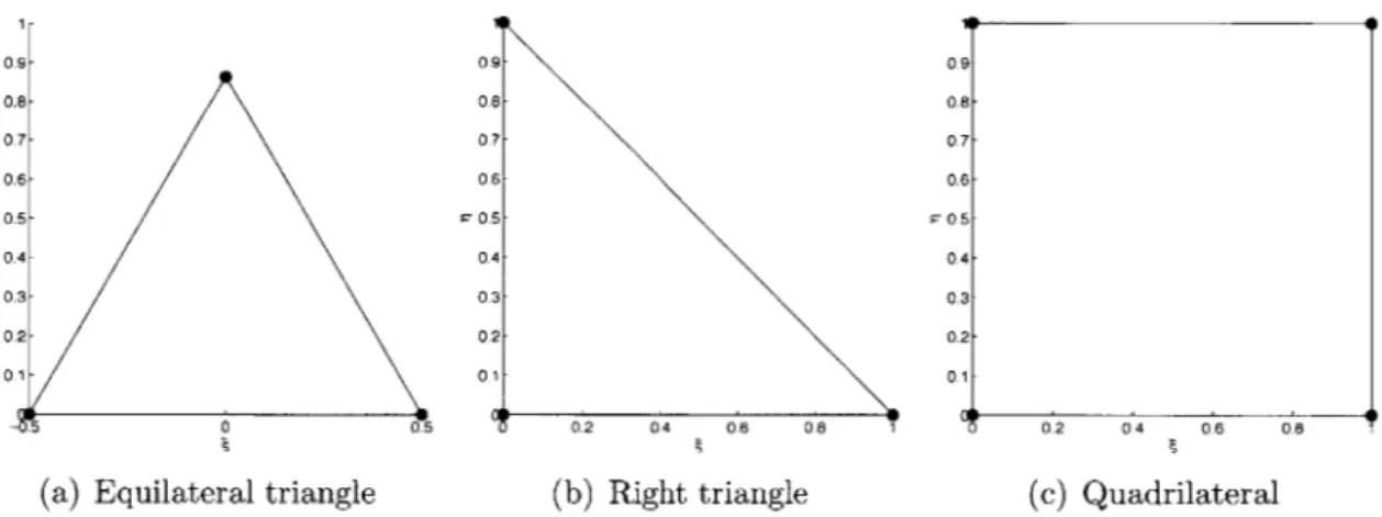
Figure 1-3: Reference shapes in two dimensions

The above analysis purely compares unit d-cubes to equilateral d-simplices. It is interesting to note, however, that right triangles and right tetrahedra reduce the num-ber of elements required to fill Q while introducing structure to the mesh, assuming the legs of the right simplices have unit length. For reference, the assumed shapes of equilateral triangles, right triangles and quadrilaterals in a two-dimensional reference

space are shown in Fig. 1-3.

Since the connectivity for both equilateral and right triangles is identical (d 2),

the memory cost of all discretisations with these shapes differ only by the area ratio, 2//, which states that right triangular meshes are always less costly than equilat-eral ones at all solution orders. In three dimensions, the assumed connectivities for equilateral and right tetrahedral meshes are different. The cost of using equilateral tetrahedra versus right tetrahedra is shown in Fig. 1-2. Only the purely discontinuous discretisations (DG, HDG) exhibit the same behaviour observed in two dimensions. That is, the cost of using equilateral versus right tetrahedra differs only by the volume

ratio,

V/'.

---I " PDE 9 Solution " Geometry ye Output " Output 9 Error L Cost estimate no

Figure 1-4: Adaptive simulation framework

1.2

Outline

Chapter 2 first presents the algorithm used to compute the mesh-adapted solution for a given computational cost. Next, Chapter 3 develops an anisotropic mixed-element mesh generation algorithm. Numerical experiments in Chapter 4 both verify and demonstrate, through applications drawn from computational fluid dynamics, the ef-fectiveness of the developed algorithm. Some conclusions and recommendations for

future work are made in Chapter 5.

For reference, the adaptive simulation framework used in this work is shown in Fig. 1-4. In general, the algorithm takes as input: a description of the domain geometry, an output of interest, a set of governing equations and a measure of the desired computational cost prescribed by the user. The solver iterates towards a

solution by adapting the mesh to reduce the error in the output of interest. As such,

discretisation, error estimation and mesh generation techniques will be discussed. This work contributes to the Metric construction and Mesh generation blocks.

1.3

Background

1.3.1

Error estimation and adaptation

Simplex-based adaptation The importance of mesh adaptation for solving

high-order discretisations of partial differential equations has been noted in [61]; in partic-ular, anisotropic mesh adaptation has received a considerable amount of interest in the past several years [33, 35, 36, 37, 38, 39, 59, 60]. Notably, Loseille and Alauzet introduce the continuous mesh framework (Sec. 2.3.1) in which they reduce the dis-crete mesh optimization problem to that of a continuous metric optimization. They compute a requested metric directly by minimizing the continuous interpolation er-ror [34]. The current work utilizes this duality between a metric and a mesh with applications to high-order discretisations. Here, the cost-constrained error minimiza-tion problem is solved via numerical techniques as in [58, 60]. While previous work has focused solely on simplicial mesh adaptation, this work extends these adaptation techniques to mixed-element meshes.

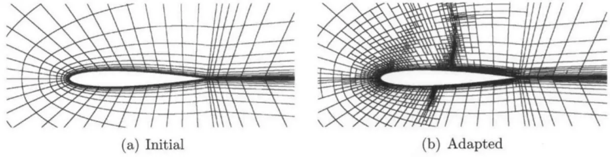
Quadrilateral subdivision Hartmann and Houston [20, 21, 22, 23] study

output-based error estimation techniques along with adaptive refinement on quadrilateral meshes. Similarly, Ceze and Fidkowski [10] build upon this work in which they per-form x, y or xy refinemenent in 2d to drive their adaptive process. It is important to note that their solver requires the treatment of hanging nodes, as shown in Fig.

1-5(b). In addition, Georgoulis et al. [17, 18] study hp-refinement strategies for

quadrilateral elements for solving second-order partial differential equations with dis-continuous Galerkin methods. They make use of the dual-weighted residual error estimate to drive h or p, isotropic or anisotropic refinement.

1.3.2

Mesh generation

Delaunay-based mesh generation Delaunay-based methods are popular for

gen-erating isotropic meshes. These methods have been implemented in softwares such as Triangle [52] in two dimensions and TetGen [53] in three dimensions. An anisotropic

(a) Initial (b) Adapted

Figure 1-5: Initial and adapted mesh obtained using the quadrilateral subdivision technique, reproduced with permission from Marco Ceze and Krzysztof J. Fidkowski

[10]

extension of the empty circumellipse property is used in the highly successful bamg (Bidimensional Anisotropic Mesh Generator) [24]. Similarly, Dobrzynski and Frey have extended the Delaunay kernel to generate anisotropic tetrahedral meshes [13].

These techniques make use of mesh modification operators, such as face swap, vertex insertion or edge collapse. The extension of these operations to cubes is chal-lenging since these operations propagate further into neighbouring elements than simplices. The analog of a circumellipse from a triangle to a quadrilateral is also poorly defined.

Advancing front mesh generation Advancing front methods [1, 32, 43, 44, 46, 50] are advantageous because they generally align elements with domain boundaries,

an attractive property when intricate mesh grading is required near geometry surfaces such as in a boundary layer. Marcum and Alauzet [1] recently presented a method for generating boundary layer meshes and creating a metric-conforming mesh in the remaining volume.

Remacle [50] uses the L' norm to generate directional, isotropic right-triangle meshes suitable for recombination into quadrilaterals. While their method appears to be fast and robust, the extension of the empty circumcircle property in the L -norm is not straightforward in the anisotropic case, let alone the extension to three

dimensions.

One striking disadvantage of the advancing front method is the arbitrary nature in which fronts collide, especially when advancing quadrilaterals directly. In the isotropic case in two dimensions, a number of heuristic smoothing and repairing techniques can be applied to repair front collisions [6, 43]. As fronts collide in the anisotropic case, metric conformity becomes an issue. Also note that mesh features may not necessarily lie near domain boundaries, such as in the case of an oblique shock wave. In these cases, fronts should ideally be setup near these metric features; a possible solution would be to use feature detection algorithms, however, this is a separate research topic and may not even extend to three dimensions.

Variational approaches Variational approaches to mesh generation consist of

pos-ing the discrete mesh generation problem as a continuous optimization problem in which some energy is minimized to compute vertex locations and mesh topology. In [30], the authors minimize the approximation error of surface quadrangulations. Also, Levy [40] introduces an approach, Vorpaline, for generating anisotropic surface

meshes. The idea is to embed both the domain

C

in R 6_{. The six-dimensional isotropic Voronoi diagram is then computed, constrained}

and projected back into R3, giving the metric-conforming triangulation of the original

surface.

They also discuss methods for generating quadrilateral and hexahedral meshes by

defining the energy of a mesh in some IP norm and optimizing this energy for the

coordinates of the constrained Voronoi tessellation [41]. They note this method has converged well for anisotropic ratios of 100:1; here, anisotropic ratios on the order of

106:1 are sought.

Primitive operations A simple method for generating metric-conforming meshes

mesh operations such as node insertion, collapse, smoothing and edge swapping to match a requested sizing and orientation field. A similar method is used by [15] where

the authors use an L norm to measure edge lengths in the reference space. Due to

their simplicity, these algorithms extend well to three dimensions, as demonstrated

by the EPIC (Edge Primitive Insertion and Collapse) code produced by The Boeing

Company [42]. Loseille [38] uses a similar approach to generate three-dimensional anisotropic meshes and also discusses the use of a boundary layer metric to add mesh

Chapter

₂

Discretization, error estimation

and adaptation

This chapter presents the adaptation algorithm used in this work, from the discreti-sation scheme to metric construction.

2.1

Numerical discretization

A general system of conservation laws within some domain Q E R d is given by

Du

a+

at

,(,X

V

with boundary conditions

B(u, Fd(U, Vu, x, t) -n; bc) = 0, Vx E OQ. (2.2)

where u(x, t) is the state vector with m components, F, denotes the convective flux,

T

d is the diffusive flux, S is a source and B is the boundary condition operator.

First, Q is tessellated into non-overlapping elements, Th, with characteristic size

space:

Vh,p = {Vh,p E [L2 h)]m

: Vh,p 0 Oqq(K) E [PP(K)] ,Vr, E Th}, (2.3)

where

#q(Ii)

mas-ter element K and PP(K) denotes the complete p-th order solution space on K.

The weak form of the governing equations are obtained by restricting u to Vh,p,

multiplying Eq. (2.1) by the test function Vh,p and integrating by parts over each

element, yielding

[V~i &Ualh~ 7Zh~p(hpiV ) 0,1 V V,p E Vh,p, (2.4)

±7hPuh

at,)

where the residual operator, lZh,p(-,-) : Vh,p x Vh,p -+ R can be broken into the

convective, diffusive and source discretizations:

C p (Uh,p,

h,pp) - 7,p (Uh,p, Vh,p) - hI,p (Uh,p, Vh,p). (2.5)

Roe's approximate Riemann solver is used to discretize the convective flux, the second form of Bassi and Rebay for the diffusive flux and the asymptotically dual-consistent form of Bassi et al. for the source term. Boundary conditions are weakly imposed by prescribing the fluxes on faces that lie on DQ. For further details of the discretisations used in this work the reader is referred to [56, 58].

2.2

Output error estimation

As highlighted in Chapter 1 the adaptation algorithm targets a specified output of

interest. In the most general setting, this output is computed by some functional

J(-) : V -± R. Denote J = J(u) as the exact output and Jh,p = Jh,p(uh,p) as the

approximated one; the error introduced by the discretisation is

Since the exact output is not known, the dual-weighted residual (DWR) method is used to estimate Eq. (2.6). This method, proposed by Becker and Rannacher [5], weights the residual operator by the adjoint solution

Strue = Rh,p(uh,p, 4) (2.7)

where 4, E W = V + Vh,P is the exact solution to the dual problem,

u,

U1,p] w, P) = -J,,[u, uh,p](w), V w E W (2.8)

where ',[u, Uh,p] : W x IN -± R and ',[u, Uhp] : W I R are the mean value

linearizations of the residual operator and output functional, respectively, defined by

r

j

Jp[U, uh,p] w)

j

where R'-,,[z](-,-) and Jhp[z](.) denote the Fr~chet derivative of R7h,p(-,-) and Jh,p(-)

with respect to the first argument evaluated about the state z.

Since the exact adjoint solution is not computable, an approximate solution,

,_{hk E Vh,k, satisfying}

Rhp[uh,p1(vh,P, 4 ,P) -- -Jp[uh,](vh,P), V Vh,P E Vh,p (2.11)

is obtained where Th is fixed but the solution space of the adjoint equation is enriched

to

P

in this work thus takes the form

8

This error can be localized over each element rK by restricting the evaluation of

Eq. (2.12) to each element,

77r

This gives an indication of the local elemental error and is useful in driving an adaptive process.

2.3

Metric construction

Now consider the problem of finding the optimal metric field to pass to the mesh generator of Chapter 3. The simplicial framework of Yano and Darmofal [58, 60], Mesh Optimization via Error Sampling and Synthesis (MOESS), is extended here to handle mixed-element meshes. First, the duality between a metric field and a mesh is discussed.

2.3.1

Mesh-metric duality,

In this work, element sizes and orientations are encoded into a Riemannian metric field which is a continuously-defined set of symmetric positive-definite (SPD) tensors defined over Q. A metric field simply transforms the notions of length and area, among other geometric properties.

Definition 2.1. (k-norm length of a vector under a metric field). The k-norm length

of a vector e e Rd in physical space under a continuous metric field,

{M(x)}

eM(e; k) =

j

(e

where A E Rd and q

E

respectively. The value of k controls the interpretation of length under a metric field and will be discussed in a later chapter. For now, assume k = 2 unless stated otherwise.

0.1 0.1

L I

Z

(a) Mesh (b) Metric

Figure 2-1: Mesh-metric duality

Definition 2.2. (volume under a metric field). The volume of a region in physical

space, r, C R , under a continuous metric field, {M(x)}xC , is given by

VM(S) = V/det(M(x)) dx. (2.15)

The above definitions alter the interpretation of edge lengths and element volumes with respect to a metric field, as shown in Fig. 2-1.

Metric-conforming mesh A tessellation,

77

vary-ing Riemannian metric field, {M (x)},,, if 77 satisfies both an edge length condition

[7, 36, 37],

fmin < eM(e) < fmax, V e E edges(Th) (2.16)

and a quality condition,

1 < q(K) < qmax, VK C E (2.17)

where the quality measure is defined in this work as

1 ZeEedges(,) 2

((e)

where CK is a constant used to assign a unit quality to the ideal reference element.

For example, cK for a unit-length equilateral triangle is 4V"5 whereas that for a unit

square is 4.

Mesh-implied metric field Given a tessellation Th, the implied metric field of Th

is defined in two steps. First, a discontinuous metric field is computed by evaluating the implied metric of each element,

fh: ([Dq(y)]T[D#4(y)]) dy

M (x) fdy V X E (2.19)

where D4q(y) is the Jacobian of the transformation from the master element to the curved element which is constant for straight-sided simplices. A continuous metric field is then constructed by averaging the metrics surrounding each mesh vertex. In the affine-invariant framework of [45], this average is computed as

argmin E log (M- 1/2_MM-1_/2₎

2 (2.20)

where

K (v)

v. The metric tensor at x can be computed by first locating the element containing

x and computing the weighted mean of the vertex metrics. In the affine-invariant framework, this is

M(x) = argmin ~ w(x)jlog (M-1/2_MM)1/2₎

2 (2.21)

where V(k) is the set of vertices on element K and w,(x) denotes the barycentric coordinate of x with respect to v. The interested reader is referred to the gradient-descent algorithm of [45] for the evaluation of Eqs. (2.20) and (2.21).

2.3.2

Mesh optimization via error sampling and synthesis

The steps needed to construct a continuous metric field during each adaptation itera-tion are now presented. This algorithm is henceforth referred to as Mesh Optimizaitera-tion via Error Sampling and Synthesis (MOESS). The method was first introduced by Yano and Darmofal [58, 60] and in this work is extended to treat mixed-element meshes. The current analysis is limited to h-adaptation; the algorithm seeks the optimal tes-sellation, 'T* of Q, given some solution order, p, which minimizes the discretization error subject to a requested computational cost,

* = arginf S(Th), s.t. C(Th) < N, (2.22) Th

where E(-) and C(.) denote the error and cost functionals, respectively. Since

simulta-neously optimizing the topology and vertex positions of Th is, in general, intractable,

the mesh-metric duality of Sec. 2.3.1 is used to apply a continuous relaxation of the optimization problem, as proposed by Loseille and Alauzet [36, 37]. As a result,

the continuous metric field

M

{M

},,

tessellation is constructed:

M* argmin 8(M) s.t. C(M) < N. (2.23)

In this view, the error and cost functionals can be evaluated as

E(M)

= (2.24)

rKETh

and

C(M) = jc,/det(M(x)) dx = c,,det M(x) dx (2.25)

where 77 is the local error indicator from Eq. (2.13). Note the constant c,,, is depen-dent on the solution order of r normalized by the size of the reference element, k.

After integration, the cost functional reduces to [58]:

C(m) = E (2.26)

where p, = dof(k) is the degrees of freedom of the reference element, k. Since high

cube-to-simplex ratio tessellations are sought, p, is set to (p + 1)d in mixed-element meshes, regardless of the element shape.

The MOESS algorithm consists of three essential stages. In Stage I, local elemental subdivisions gather metric-error pairs to be used in the construction of a metric-error model (Stage II). Stage III uses this model to optimize A4 which will be subsequently passed to the mesh generator of Chapter 3.

Stage I: Error sampling Eq. (2.13) gives a measure of the local error over an

element ;o E Th due to the discretisation. Each element, o, can be further split and

the error over each child element can be recalculated. The split configurations used in this work are shown in Figs. 2-2 and 2-3.

K0 K K2 K3 K4

(a) Original (b) Split 1 (c) Split 2 (d) Split 3 (e) Uniform

Figure 2-2: Triangle split configurations

K K K₂ K₃ K" K₅

(a) Original (b) Split 1 (c) Split 2 (d) Split 3 (e) Split 4 (f) Uniform

Figure 2-3: Quadrilateral split configurations

The implied metric associated with each split configuration is taken as the affine-invariant mean, Eq. (2.20), of the implied metrics of the child elements and the error

introduced by the child elements is summed to complete the set of metric-error pairs:

{Mf As}q,j I =' 1, ... ,* ns (2.27)

where n, denotes the number of samples used on ro.

The implied metric of each split element along with its recomputed error is used to build a list of metric-error samples. In the case of quadrilaterals, all five split configurations are used.

Stage II: Error model synthesis The metric-error pairs are then used to

con-struct a model of the error as a function of the metric field. This model is concon-structed in terms of the step tensor, S, which represents the vector difference between two metric tensors. In the context of the discrete set of sampled data, these tensors are

computed from M, and MA, 0 as

= log

(Mi/

A linear model is then constructed from the n. metric-error samples,

f,(S)

where R, is referred to as the rate tensor. A linear regression of the sampled data is used to determine R,. Note the importance of the diagonal splits of Fig. 2-3. For the case of parallelograms, the step tensor implied by the uniform refinement configuration is a linear combination of those implied by the two anisotropic splits, thus causing the regression to be underdetermined. The diagonal samples encode additional information into the error model synthesis and prevent such a failure.

Stage III: Metric optimization Equipped with an error model over each element,

which yields the requested metric at each element vertex. Recent work by [28] has investigated the use of gradient-based techniques to solve Eq. (2.23). The original formulation is supplemented with constraints to limit the change in the mesh during each adaptation. Denoting the field of step tensors as S, the problem formulation is stated as follows: S= arginf S(S) + pq

(

where the penalty term is defined as O(z) = (z < 0) ?0 : z2 _{and n" is the number of} vertices in Th. The penalty vector, p is used to control edge length deviations and the user-specified refinement factor, r, is used to control the change in the mesh from one adaptation to the next. The optimization problem is solved as follows. First, p is initialized to some constant c and the initial problem is solved using the Method of Moving Asymptotes in the optimization library, NLopt [27]. For the resultant step tensors which do not satisfy the edge length condition, the corresponding entry in p is multiplied by some constant factor, /, to further penalize that step tensor. In the

Chapter 3

Mesh generation

This chapter presents the algorithm used to generate metric-conforming, mixed-element meshes. Curvilinear mesh generation is also discussed.

ursa

--- I

" eti eld -eMs

Figure 3-1: Mesh generation algorithm

3.1

Fundamentals

A basic outline of the mesh generation algorithm used in this work is shown in Fig. 3-1.

The output mesh is generated from a given geometry and metric field in a dimension-by-dimension approach. The problem of generating metric-conforming surface meshes is first treated and followed by a volume tessellation algorithm. The straight-sided mesh is then curved, as required by the high-order finite-element solver. The devel-oped mesh generation package will be henceforth referred to as ursa (unstructured

anisotropic). Some central ideas used throughout ursa are first discussed.

3.1.1

Geometry representation

The input geometry takes the form of a Non-Uniform Rational B-Spline (NURBS). Several geometric algorithms including evaluation, differentiation, projection and interpolation were drawn from The ArURBS Book [48]. The basic form of a d-dimensional NURBS curve is

E Ni,p(u)wiPi

x(U) = i=, a < u < b. (3.1)

E Ni, (u) wi

i=O

where P E R n x Rd is the vector of control points, w E Rn is the vector of weights

and NP E R n is the p-th degree B-Spline basis functions, defined over some interval

in the knot vector, ii. In the current implementation, a set of points along the true geometry is interpolated with cubic NURBS curves. In this setting, the knot vector is computed using the chord length method of [48] and the weights are set to 1, recovering cubic B-Splines.

3.1.2

Metric field evaluation

The input metric field can be described either analytically or, more practically, through the use of a background tessellation. Upon initial import, the input tes-sellation is split, such that no quadrilateral elements remain in the background mesh.

This has little effect on the evaluation of

M

of the background mesh. Evaluation of the metric tensor at x is done by first lo-cating the element containing x, computing the barycentric weights with respect to the three triangle vertices and interpolating the nodal metrics, as in Eq. (2.21). An efficiency gain is made by storing the background enclosing shape for each active node during the mesh generation algorithm. This reduces the triangle search time to approximately 0(1) as the algorithm converges.

3.1.3

Right triangle mesh generation

The proposed algorithm for generating mixed-element tessellations first consists in creating a right-triangle mesh and further combining pairs of right triangles into quadrilaterals, when possible.

Lk norm

Traditional mesh generation algorithms, such as [24] and [42] aim for unit equilateral simplices. In particular Edge Primitive Insertion and Collapse (EPIC) [42] makes use of simple mesh operations, driven by edge length and element quality calculations, to generate a mesh.

1.41421 1.09051 1

1 1 1

1 1 1

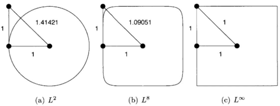
(a) L2 (b) L8 (c) L

Figure 3-2: Interpretation of a right triangle with respect to a unit Lk ball

The Lk norm modifies how lengths are interpreted in the reference metric space. Equilateral simplex mesh generation algorithms should be thought of as L2-based algorithms. Here, the L' norm is proposed to create right triangles; this idea was previously investigated by [41, 50, 15]. The length of an edge under a d-dimensional metric field can be computed in a k-norm from Eq. (2.14). Here, the two metric tensors defined at the end nodes of an edge are averaged in the affine-invariant sense to reduce the integration in Eq. (2.14) to a single evaluation. All three edge lengths of a right triangle approach unity as k approaches infinity, as depicted in Fig. 3-2. It should be noted that the quality of an element under M given by Eq. (2.18) is only

Recombination algorithms

Once a right triangle mesh is generated, pairs of triangles can be combined to form quadrilateral elements. Previous work includes the simple merging procedure of [8] or graph-matching algorithms; the latter is adopted as was done in [19, 50] and make use of the Blossom IV algorithm [11, 12]. The underlying principle of the recombination algorithm is that a triangulation is simply a graph, where each triangle is a graph node and each triangle-neighbour pair is an edge in the graph, as shown in Fig. 3-3.

blossom

Figure 3-3: Graph-matching approach

The Blossom IV algorithm computes a minimum-weight perfect matching of an input graph and allows the assignment of weights, w, to the triangle-neighbour pairs. Here, the weights are assigned as

W(K1, K2) = o-({det Do1,i}) (3.2)

where ni and K2 are the proposed pair of triangles, o is the standard-deviation function

and D01,j represents the Jacobian of the bilinear shape functions (q = 1) at some i-th

sample point. Here, the coordinates of a tenth-order quadrature rule is used to sample the Jacobian of the proposed quadrilateral. This weighting function has been chosen to penalize elements with significantly-varying Jacobians. That is, parallelograms are sought because they have constant Jacobians and thus, constant implied metric tensor

M(u3) M(U2) M(ui)

M)(U4)

Figure 3-4: Curve metric description with true geometry

which is believed to enhance the fidelity of the error modeling stage of Sec. 2.3.2.

3.2

Surface mesh generation

The first step in generating a metric-conforming mesh is to tessellate the input

ge-ometry in forming !g = 0Th. The background mesh provides nodal metrics along the

domain boundaries, which are used to construct a one-dimensional background mesh in the parameter space of the corresponding NURBS curve, see Fig. 3-4.

The algorithm begins by integrating the metric along the geometry,

EM(F)

= iM(yi) = E

]

i=1 i=-1

Note the use of the L2 _{norm in this computation which aligns quadrilateral edges with}

the geometry instead of its diagonals. The number of edges needed to discretise the geometry is then n' = round(em(F)). Each inserted edge should then have a length of

A'4 (F) (3.4)

ne

Parameter values are then determined through a linear interpolation of the accumu-lated edge lengths of Eq. (3.3); Eq. (3.1) is then evaluated to obtain the physical coordinates of the surface nodes.

3.3

Volume mesh generation

The volume mesh generation algorithm was influenced by the work of [15] and in-volves an iterative sequence of primitive mesh operations. In particular, edge split, edge collapse, node relocation and edge swap operators are used, as shown in Fig. 3-6. Operations are only performed if the worst quality of the affected (dark gray) trian-gles is improved by the operation, inspired by the work of [29]. This requirement is relaxed for the node relocation operator and element areas are simply checked to remain positive during the relocation.

The volume mesh generation algorithm is described in Alg. 1. Note that all

length and quality computations are performed in M. The aspect ratio function is

computed from the eigenvalues, A, of M as, A = V/Amax/Amin and are sorted in

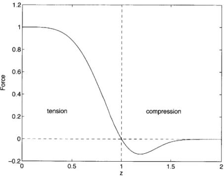
decreasing order to target regions of high anisotropy first. The relocate function acts as a smoother during the iterative process. Similar to [9] and [15], the force on each node is computed from the L' norm edge length:

f(v) =

E

ecedges(v)

where q* is the eigenvector of

M(x(v))

-z') exp(-z) which applies a tensile force to short edges and a compressive force for

long edges as shown in Fig. 3-5. Note that this field is stronger for shorter edges rather than longer edges since edge splits are always valid whereas edge collapses can sometimes introduce inverted elements. Thus, a stronger force is needed to improve the possibility of elongating short edges. The swaptimize function seeks the optimal swap configuration about a node star or element neighbours which will improve the worst quality of the affected elements, if possible. The parameters used here are

1

Algorithm: Th <- (gh, M)

Th <- _{triangulation of nodes on surface mesh,} g!.

while not converged do

Tag RA(M(x(v))) at all nodes v E Th and sort.

for v E Th do

relocate(v)

e +- shortest edge attached to v

/i <- opposite node to v on e

if fM(e) < lmin and col lapse(v, vi) improves worst quality then

collapse(, vi)

swaptimize(v) else

e <- longest edge attached to v vi +- opposite node to v on e

if fM(e) > lm, and sp lit (v, v1) improves worst quality then

split

(v,

Perform ni iterations of smoothing on all nodes.

Perform n2 iterations of swaptimization on all nodes.

1.2 1 (D P 0 UL 0.8 0.6 0.4 0.2 0 -n 0

Figure 3-5: Force used under a metric field

0.5 1

z

1.5 2

to elongate or compress mesh edges according to their length

3.4

Curvilinear mesh generation

For problems with curved boundaries, a high-order representation of the geometry is required [4]. In this work, a nonlinear elastic model is used to generate curvilinear meshes [42, 47]. Denote the desired coordinates of the deformed, high-order nodes as x and those in the reference, undeformed, volume as xo. The sensitivity of the deformed volume with respect to the initial configuration is

(3.6)

F =Ox

Oxo

where F is the deformation gradient tensor. Imposing a force equilibrium on an arbi-trary volume and applying the divergence theorem yields the equilibrium condition

V - P = 0, _(3.7)

tension compression