HAL Id: tel-02890430
https://tel.archives-ouvertes.fr/tel-02890430
Submitted on 6 Jul 2020HAL is a multi-disciplinary open access archive for the deposit and dissemination of sci-entific research documents, whether they are pub-lished or not. The documents may come from teaching and research institutions in France or abroad, or from public or private research centers.
L’archive ouverte pluridisciplinaire HAL, est destinée au dépôt et à la diffusion de documents scientifiques de niveau recherche, publiés ou non, émanant des établissements d’enseignement et de recherche français ou étrangers, des laboratoires publics ou privés.
Modeling and scheduling embedded real-time systems
using Synchronous Data Flow Graphs
Jad Khatib
To cite this version:
Jad Khatib. Modeling and scheduling embedded real-time systems using Synchronous Data Flow Graphs. Embedded Systems. Sorbonne Université, 2018. English. �NNT : 2018SORUS425�. �tel-02890430�
TH`ESE DE DOCTORAT DE SORBONNE UNIVERSIT´E
Sp´ecialit´e Informatique ´
Ecole doctorale Informatique, T´el´ecommunications et ´Electronique (Paris)
Pr´esent´ee par
Jad KHATIB
Pour obtenir le grade de
DOCTEUR de SORBONNE UNIVERSIT´E
Sujet de la th`ese :
Mod´
elisation et ordonnancement des syst`
emes temps r´
eel
embarqu´
es utilisant des graphes de flots de donn´
ees synchrones
Modeling and scheduling embedded real-time systems using Synchronous Data Flow Graphs
soutenue le 11 septembre 2018 devant le jury compos´e de :
Mme. Alix Munier-Kordon Directrice de th`ese Mme. Kods Trabelsi Encadrante de th`ese M. Fr´ed´eric Boniol Rapporteur
M. Pascal Richard Rapporteur M. Laurent George Examinateur M. Lionel Lacassagne Examinateur M. Dumitru Potop-Butucaru Examinateur M. Etienne Borde Examinateur
Acknowledgements
I would like to take the opportunity to thank all those who supported me during my thesis.
I have an immense respect, appreciation and gratitude towards my advisors: Ms. Alix Munier-Kordon, Professor at Sorbonne Université, and Ms. Kods Trabelsi, Research Engineer at CEA LIST, for their consistent guidance and support during my thesis journey. I would like to thank them for sharing their invaluable knowledge, experience and advice which have been greatly beneficial for the successful completion of this thesis. I would like to extend my sincere gratitude to the reviewers, Professor Frédéric Boniol and Professor Pascal Richard for accepting to evaluate my thesis. My earnest thanks are also due to Professor Laurent George, Professor Lionel Lacassagne, Doctor Dumitru Potop-Butucaru and Doctor Etienne Borde for accepting to be a member of the jury. Thanks to all Lastre and LCE team members for the occasional coffees and discussions especially during our “PhD Days”. Thanks also to my colleagues in Lip6 and Télécom Paristech: Youen, Cédric, Eric, Olivier, Roberto and Kristen as well as all those I forgot to mention.
I would also like to thank my friends Sarah, Laure, Marcelino, Hadi, Serge and Damien for their support and all our happy get-togethers and for uplifting my spirit during the challenging times faced during this thesis.
I am particularly grateful to my friend Catherine for her priceless friendship and precious support and for continuously giving me the courage to make this thesis better. Last but definitely not least, I am forever in debt to my awesomely supportive mother Zeina and my wonderful sister Jihane for inspiring and guiding me throughout the course of my life and hence this thesis.
Résumé
Les systèmes embarqués temps réel impactent nos vies au quotidien. Leur com-plexité s’intensifie avec la diversité des applications et l’évolution des architectures des plateformes de calcul. En effet, les systèmes temps réel peuvent se retrouver dans des systèmes autonomes, comme dans les métros, avions et voitures autonomes. Ils sont donc souvent d’une importance décisive pour la vie humaine, et leur dysfonction-nement peut avoir des conséquences catastrophiques. Ces systèmes sont généralement multi-périodiques car leurs composants interagissent entre eux à des rythmes différents, ce qui rajoute de la complexité. Par conséquent, l’un des principaux défis auxquels sont confrontés les chercheurs et industriels est l’utilisation de matériel de plus en plus complexe, dans le but d’ exécuter des applications temps réel avec une performance optimale et en satisfaisant les contraintes temporelles. Dans ce contexte, notre étude se focalise sur la modélisation et l’ordonnancement des systèmes temps réel en utilisant un formalisme de flot de données. Notre contribution a porté sur trois axes:
Premièrement, nous définissons un mode de communication général et intuitif au sein de systèmes multi-périodiques. Nous montrons que les communications entre les tâches multi-périodiques peuvent s’exprimer directement sous la forme d’une classe spécifique du “Synchronous Data Flow Graph” (SDFG). La taille de ce graphe est égale à la taille du graphe de communication. De plus, le modèle SDFG est un outil d’analyse qui repose sur de solides bases mathématiques, fournissant ainsi un bon compromis entre l’expressivité et l’analyse des applications.
Deuxièmement, le modèle SDFG nous a permis d’obtenir une définition précise de la latence. Par conséquent, nous exprimons la latence entre deux tâches communicantes à l’aide d’une formule close. Dans le cas général, nous développons une méthode d’évaluation exacte qui permet de calculer la latence du système dans le pire des cas. Ensuite, nous bornons la valeur de la latence en utilisant deux algorithmes pour calculer les bornes inférieure et supérieure. Enfin, nous démontrons que les bornes de la latence peuvent être calculées en temps polynomial, alors que le temps nécessaire pour évaluer sa valeur exacte augmente linéairement en fonction du facteur de répétition moyen.
Finalement, nous abordons le problème d’ordonnancement mono-processeur des systèmes strictement périodiques non-préemptifs, soumis à des contraintes de
com-vi
munication. En se basant sur les résultats théoriques du SDFG, nous proposons un algorithme optimal en utilisant un programme linéaire en nombre entier (PLNE). Le problème d’ordonnancement est connu pour être NP-complet au sens fort. Afin de résoudre ce problème, nous proposons trois heuristiques: relaxation linéaire, simple et ACAP. Pour les deux dernières heuristiques, et dans le cas où aucune solution faisable n’est trouvée, une solution partielle est calculée.
Mots clés: systèmes temps réel, graphes de flots de données synchrones, modélisation
des communications, tâches strictement périodiques non-préemptifs, ordonnancement mono-processeur, latence.
Abstract
Real-time embedded systems change our lives on a daily basis. Their complexity is increasing with the diversity of their applications and the improvements in processor architectures. These systems are usually multi-periodic, since their components commu-nicate with each other at different rates. Real-time systems are often critical to human lives, their malfunctioning could lead to catastrophic consequences. Therefore, one of the major challenges faced by academic and industrial communities is the efficient use of powerful and complex platforms, to provide optimal performance and meet the time constraints. Real-time system can be found in autonomous systems, such as air-planes, self-driving cars and drones. In this context, our study focuses on modeling and scheduling critical real-time systems using data flow formalisms. The contributions of this thesis are threefold:
First, we define a general and intuitive communication model within multi-periodic systems. We demonstrate that the communications between multi-periodic tasks can be directly expressed as a particular class of “Synchronous Data Flow Graph” (SDFG). The size of this latter is equal to the communication graph size. Moreover, the SDFG model has strong mathematical background and software analysis tools which provide a compromise between the application expressiveness and analyses.
Then, the SDFG model allows precise definition of the latency. Accordingly, we express the latency between two communicating tasks using a closed formula. In the general case, we develop an exact evaluation method to calculate the worst case system latency from a given input to a connected outcome. Then, we frame this value using two algorithms that compute its upper and lower bounds. Finally, we show that these bounds can be computed using a polynomial amount of computation time, while the time required to compute the exact value increases linearly according to the average repetition factor.
viii
Finally, we address the mono-processor scheduling problem of non-preemtive strictly periodic systems subject to communication constraints. Based on the SDFG theoretical results, we propose an optimal algorithm using MILP formulations. The scheduling problem is known to be NP-complete in the strong sense. In order to solve this issue, we proposed three heuristics: linear programming relaxation, simple and ACAP heuristics. For the second and the third heuristic if no feasible solution is found, a partial solution is computed.
Keywords: real-time systems, Synchronous Data Flow Graph, communications
Table of contents
List of figures xiii
List of tables xvii
Table of Acronyms xix
1 Introduction 1
1.1 Contributions . . . 2
1.2 Thesis overview . . . 3
2 Context and Problems 5 2.1 Real-time systems . . . 6
2.1.1 Definition . . . 6
2.1.2 Real-Time systems classification . . . 7
2.1.3 Real-time tasks’ characteristics . . . 8
2.1.4 Tasks models . . . 10
2.1.5 Execution mode . . . 11
2.1.6 Communication constraints . . . 12
2.1.7 Latency . . . 13
2.1.8 Multi-periodic systems . . . 13
2.2 Problems 1 & 2: Modeling multi-periodic systems and evaluating their latencies . . . 14
2.3 Modeling real-time systems . . . 15
2.3.1 Models for Real-Time Programming . . . 16
2.3.2 Low-level languages . . . 19
2.3.3 Synchronous languages . . . 19
2.3.4 Oasis . . . 23
2.3.5 Matlab/Simulink . . . 24
x Table of contents
2.4 Scheduling real-time system . . . 26
2.5 Problem 3: Scheduling strictly multi-periodic system with communica-tion constraints . . . 29
2.6 Conclusion . . . 30
3 Data Flow models 31 3.1 Data Flow Graphs . . . 31
3.1.1 Kahn Process Network . . . 32
3.1.2 Computation Graph . . . 32
3.1.3 Synchronous Data Flow Graph . . . 33
3.1.4 Cyclo-Static Data Flow Graph . . . 35
3.2 Synchronous Data Flow Graph Characteristics and transformations . . 36
3.2.1 Precedence relations . . . 36
3.2.2 Consistency . . . 38
3.2.3 Repetition vector . . . 39
3.2.4 Normalized Synchronous Data Flow graph . . . 40
3.2.5 Expansion . . . 41
3.3 Conclusion . . . 44
4 State of art 45 4.1 Modeling real time systems using data flow formalisms . . . 45
4.1.1 Latency evaluation using data flow model . . . 47
4.1.2 Main difference . . . 48
4.2 Scheduling strict periodic non-preemptive tasks . . . 49
4.2.1 Preemptive uniprocessor schedulability analysis . . . 49
4.2.2 Scheduling non-preemptive strictly periodic systems . . . 51
4.3 Conclusion . . . 55
5 Real Time Synchronous Data Flow Graph (RTSDFG) 57 5.1 modeling real time system communications using RTSDFG . . . 58
5.1.1 Periodic tasks . . . 58
5.1.2 Communication constraints . . . 59
5.1.3 From real time system to RTSDFG model . . . 62
5.2 Evaluating latency between two periodic communicating tasks . . . 66
5.2.1 Definitions . . . 67
5.2.2 Maximum latency between two periodic communicating tasks . 70 5.2.3 Minimum latency between two periodic communicating tasks . . 72
Table of contents xi
5.3 Evaluating the worst-case system latency . . . 74
5.3.1 Definition . . . 74
5.3.2 Exact pricing algorithm . . . 76
5.3.3 Upper bound . . . 84
5.3.4 Lower bound . . . 87
5.4 Conclusion . . . 89
6 Scheduling strictly periodic systems with communication constraints 91 6.1 Scheduling a strictly periodic independent tasks . . . 92
6.1.1 Strictly periodic tasks . . . 92
6.1.2 Schedulabilty analysis of strictly periodic independent tasks . . 94
6.2 Synchronous Data Flow Graph schedule . . . 97
6.2.1 As Soon As Possible schedule . . . 97
6.2.2 Periodic schedule . . . 98
6.3 Schedulabilty analysis of two strictly periodic communicating tasks . . 99
6.4 Optimal algorithm: Integer linear programming formulation . . . 104
6.4.1 Fixed intervals . . . 105
6.4.2 Flexible intervals . . . 108
6.5 Heuristics . . . 113
6.5.1 Linear programming relaxation . . . 113
6.5.2 Simple heuristic . . . 115
6.5.3 ACAP heuristic . . . 119
6.6 Conclusion . . . 131
7 Experimental Results 133 7.1 Graph generation: Turbine . . . 133
7.2 Latency evaluation . . . 134
7.2.1 Computation time . . . 135
7.2.2 Quality of bounds . . . 136
7.3 Mono-processor scheduling . . . 138
7.3.1 Generation of tasks parameters . . . 138
7.3.2 Optimal algorithm . . . 139
7.3.3 Heuristics . . . 149
7.4 Conclusion . . . 157
8 Conclusion and Perspectives 159
List of figures
2.1 Schematic representation of a real-time system. . . 7
2.2 Real-time tasks’ characteristics. . . 9
2.3 Liu and Layland model. . . 10
2.4 Example of a harmonic multi-periodic system. . . 14
2.5 Execution of an asynchronous model. . . 16
2.6 Execution of a timed model. . . 17
2.7 Execution of a synchronous model. . . 18
3.1 Example of Kahn Processor Network. . . 32
3.2 Example of Computation Graph. . . 33
3.3 A simple example of Synchronous Data Flow Graph. . . 34
3.4 An example of a Cyclo-Static Data Flow Graph. . . 35
3.5 Cyclic Synchronous Data Flow Graph. . . 39
3.6 Example of Synchronous Data Flow Graph normalisation. . . 41
3.7 Example of a SDFG transformation into equivalent HSDFG using the technique introduced by Sih and Lee [108]. . . 42
3.8 Example of SDFG transformation into equivalent HSDFG using the expansion. . . 44
5.1 Liu and Layland model . . . 58
5.2 Simplification of Liu and layland’s model . . . 60
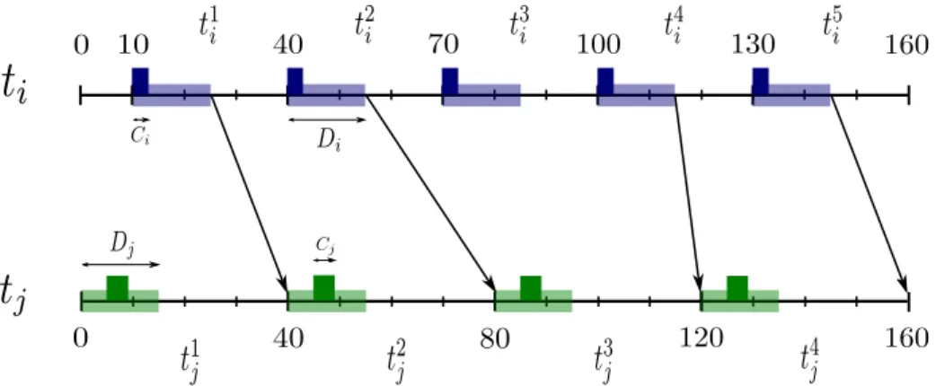
5.3 Example of multi-periodic communication model . . . 61
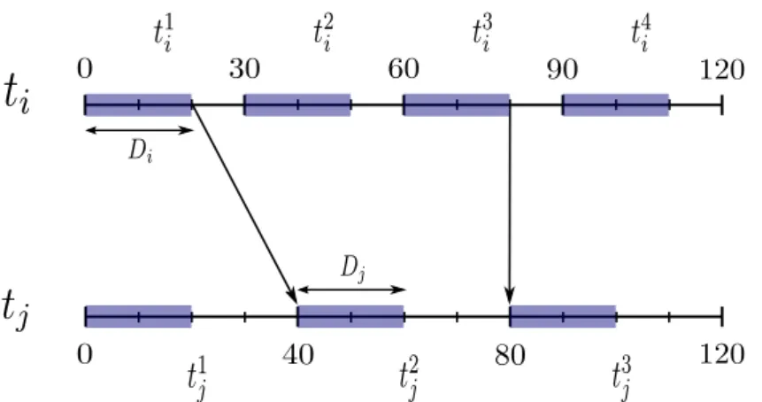
5.4 The Buffer a = (ti, tj) that models the communication constraints be-tween the tasks executions of the example illustrated in Figure 5.3. . . 64
5.5 An example of scheduling which respects the communication constraints between the tasks ti= (0,5,20,30) and tj= (0,10,20,40). . . 65
xiv List of figures
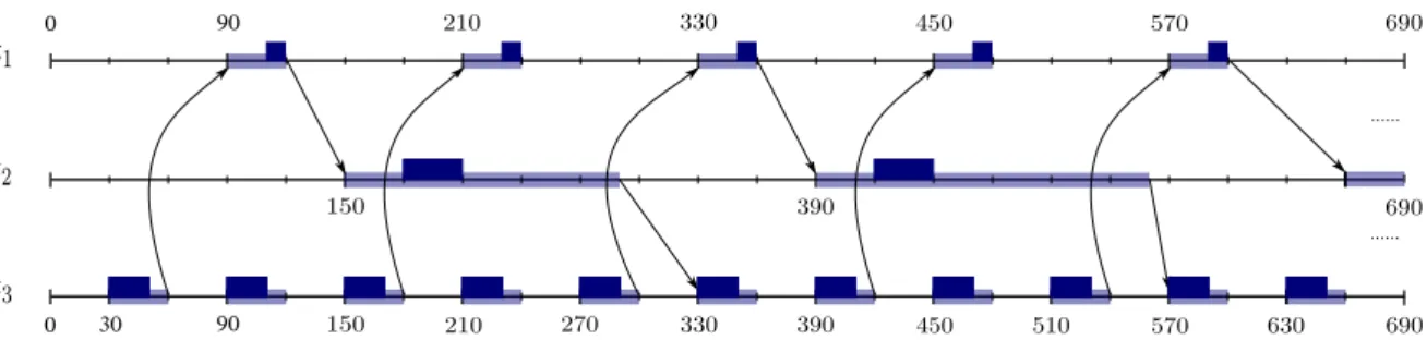
5.7 The RTSDFG that models the communications between the tasks’ executions of the multi-periodic system presented in Table 5.1 and Figure 5.6 . . . 66 5.8 Example of communication scheme between two periodic communicating
tasks. . . 68 5.9 Path pth = {t1, t2, t3} which corresponds to the communication graph
of three periodic tasks. . . 75 5.10 Communication and execution model of the path pth = {t1, t2, t3}
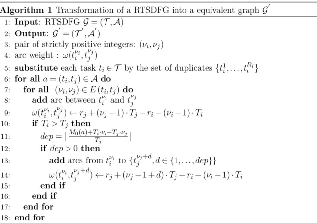
de-picted in Figure 5.9. . . 75 5.11 RTSDFG G = (T ,A) modeling the communication constraints between
the tasks’ executions of the example represented in Figure 5.10. . . 79 5.12 Graph G′ = (T′, A′) that models precedence and dependency constraints
between the tasks executions of the RTSDFG depicted in Figure 5.11. . 80 5.13 Computation of the Worst-case latency of the RTSDFG depicted in
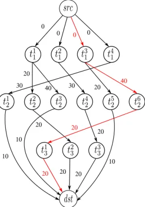
Figure 5.11. . . 82 5.14 A cyclic RTSDFG with its equivalent graph that models the precedence
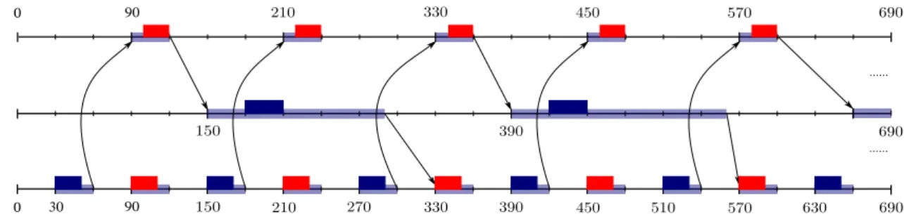
and dependence constraints between the tasks executions. . . 83 5.15 Example of latency upper bound computation using the weighted graph
Gmax . . . 87
5.16 Latency lower bound computation of the RTSFDG depicted in Figure 5.15a using the weighted graph Gmin. . . . 88
6.1 Non-preemptive strictly periodic task. . . 93 6.2 Scheduling two strictly periodic tasks ti= (0,5,30) and tj= (5,5,40) on
the same processor. . . 95 6.3 Example of a SDFG and its ASAP schedule. . . 97 6.4 A feasible periodic schedule of the SDFG depicted in Figure 6.3a. . . . 99 6.5 Communications constraints between the executions of two strictly
periodic tasks ti= (10,3,15,30) and tj= (0,4,15,40). . . 100
6.6 Scheduling two strictly periodic communicating tasks on the same pro-cessor. . . 102 6.7 RTSDFG G = (T ,A). . . 107 6.8 A feasible Schedule of a strictly periodic system with communication
constraints. . . 107 6.9 Example of an infeasible solution where the resource constraints are not
fulfilled. There is an overlapping between the executions of t1 and that
List of figures xv
6.10 A feasible schedule of the example depicted in Figure 6.9. Communica-tion constraints are respected and there is no overlapping between the tasks executions. . . 110 6.11 RTSDFG G = (T ,A) modeling the communication constraints between
the executions of t1= (110,10,25,120), t2 = (15,15,30,60) and t3=
(190,45,200,240). . . 111 6.12 Communication scheme between the executions oft1= (110,10,25,120),
t2= (15,15,30,60) and t3= (190,45,200,240). . . 112
6.13 Scheduling the strictly periodic communicating tasks t1= (110,10,25,120),
t2= (15,15,30,60) and t3= (190,45,200,240) on the same processor. . . 112
6.14 A feasible solution for the scheduling problem is obtained by solving the new LP. . . 115 6.15 RTSDFG G = (T ,A). . . 117 6.16 A feasible schedule of the strictly periodic system represented in Table
6.2 and Figure 6.15. The tasks starting dates are respectively equal to
s1= 0,s2= 8 and s3= 4. . . 118
6.17 A Partial solution of the scheduling problem using Algorithm 4. The tasks starting dates are respectively equal to s1= 10 and s3= 40. . . . 119
6.18 Scheduling task t2= (120,10,50,144) at the end of the execution of task
t1= (10,4,10,18) which is already scheduled. . . 121
6.19 Scheduling task t2= (120,10,50,144) such that the end of its execution
corresponds to the beginning of task t1= (10,4,10,18) which is already
scheduled. . . 121 6.20 A feasible schedule resulting from applying Algorithm 5 on the perioidic
system. . . 124 6.21 RTSDFG G = (T ,A). . . 129 6.22 A feasible schedule of the strictly periodic system represented in Table
6.3 and Figure 6.21. . . 131 7.1 Average latency value using the evaluation methods with respect to the
graph size |T |.The average repetition was fixed to 125. . . 136 7.2 Deviation ratio between the latency exact value and its bounds. . . 137 7.3 MILP acceptance ratio on harmonic tasks generated with different
periods ratios. . . 140 7.4 Experimental results on harmonic instances of RTSDFGs with different
xvi List of figures
7.5 Experimental results on harmonic and non-harmonic instances with different system utilizations. . . 143 7.6 MILP acceptance ratio on harmonic acyclic and cyclic instances with
respect to the system utilization. . . 144 7.7 Experimental results on harmonic instances for fixed and flexible cases. 145 7.8 Percentage of solver failure instances for fixed and flexible cases with
respect to the system utilization. . . 146 7.9 Percentage of solver failure instances for flexible case with respect to the
graph size. . . 147 7.10 Experimental results on harmonic instances with and without release
dates. . . 148 7.11 Experimental results on harmonic instances without release dates. . . . 150 7.12 Average computation time to find a feasible solution. . . 151 7.13 Results obtained by applying our heuristics on the solver failure instances.152 7.14 Partial solutions: percentage of tasks that can be scheduled on the same
processor. . . 153 7.15 Experimental results on harmonic instances with release dates. . . 154 7.16 Average computation time to find a feasible solution. . . 155 7.17 The mega-heuristic acceptance ratio on harmonic instances without
release dates. The RTSDFG size |T | was fixed to 30 tasks. . . 156 7.18 The mega-heuristic acceptance ratio on harmonic instances with release
List of tables
2.1 Lustre program behaviour. . . 21
5.1 Periodic tasks parameters . . . 66
6.1 Strictly periodic tasks parameters . . . 107
6.2 Strictly periodic tasks parameters . . . 117
6.3 Strictly periodic tasks parameters . . . 129
7.1 Average computation time of latency evaluation methods for Huge RTSDFGs with respect to their average repetition factors. . . 135
7.2 Average computation time of latency evaluation methods for RTSDFGs according to their size |T |. . . 135
7.3 Average computation time of latency evaluation methods for RTSDFGs according to their size |T |. . . 136
Table of Acronyms
ACAP As Close As Possible
ADL Architecture Description Language API Application Programming Interface ASAP As Soon As Possible
CAN Controller Area Network CP Computation Graph CPU Central Processing Unit
CSDFG Cyclo-Static Dataflow Graph
DAG Directed Acyclic Graph DM Deadline Monotonic DP Dynamic Priority
DPN Dataflow Process Network EDF Earliest Deadline First E/E Electric/Electronic FIFO First-In-First-Out
GCD Greatest Common Divisor
HSDFG Homogeneous Synchronous Data Flow
xx List of tables I/O Input/Output
KPN Kahn Process Network LCM Least Common Multiple LET Logical Execution Time LP Linear Programming
MILP Mixed Integer Linear Programming MPPA Massively Parallel Processor Array NoC Network on Chip
OS Operating System
PGM Processing Graphs Methods RBE Rate Base Execution
RM Rate Monotonic
RTA Response Time Analysis RTOS Real-Time Operating System
RTSDFG Real-Time Synchronous Data Flow Graph
SBD Synchronous Block Diagrams SDFG Synchronous Data Flow Graph SWC Software Component
TTA Time Triggered Architectures WCET Worst Case Execution Time WCRT Worst Case Response Time
Chapter 1
Introduction
Nowadays, electronic devices are ubiquitous in our daily lives. Every time we set an alarm, drive a car, take a picture or use a cell-phone, we interact in some way with electronic components or devices. Electronic systems make people’s lives safer, faster, easier and more convenient. These systems, integrated in a larger environment with specific assignments or purposes, are called embedded systems. They comprise a hardware part (electronic) that defines interfaces and system performance as well as a software part (computer) that dictates their functions. Such systems are autonomous and limited in size, power consumption, and heat dissipation. In order to achieve specific tasks, their design combines skills from computer and electronics fields.
An important class of embedded systems is real-time embedded systems. They operate dynamically in their environments and must continuously adapt to their changes. Indeed, they fully command their environments through actuators upon data reception via sensors. The correctness of such systems depends not only on the logical result but also on the time it is delivered. Therefore, real-time systems are classified according to the temporal constraints severity: soft, firm and hard (critical) systems. In hard systems, the violation of a temporal constraint can lead to catastrophic consequences. The aircraft piloting system, the control of a nuclear power plant and the track control system are typical examples. The soft and firm systems are more “tolerant”: the temporal constraint violation does not cause serious damages to the environment and does not corrupt the system behaviour. In fact, this violation leads to a degradation of the result quality (i.e performance).
On the other hand, critical real-time systems are becoming increasingly complex. They require research effort in order to be effectively modeled and executed. In this context, one of the major challenges faced by academic and industrial environments is the efficient use of powerful and complex resources, to provide optimal performance
2 Introduction
and meet the time constraints. These systems are usually multi-periodic, since their components communicate with each other at different rates. This is mainly due to their physical characteristics. For this reason, a deep analysis of communications within multi-periodic systems is required. This analysis is essential to schedule these systems on a given platform. Moreover, the estimation of parameters in a static manner, such as evaluating the latency between the system input and its corresponding outcomes, is an important practical issue.
1.1
Contributions
In this section, we summarize the research contribution of this thesis.
The first contribution consists in defining a general and intuitive communication model for multi-periodic systems. Based on the precedence constraints between the tasks executions, we demonstrate that the communications between multi-periodic tasks can be directly expressed as a “Synchronous Data-flow Graph”. The size of this graph is equal to the application size. We called this particular class “Real-Time Synchronous Data-flow Graphs”. These results were published in a short paper in “Ecole d’été temps réel”(ETR 2015). In collaboration with Cedric Klikpo (projet ELA, IRT SystemX), we showed that the communications of an application expressed with Simulink can be modeled by a SDFG. This transformation led to an article published in RTAS 2016 [76]. The second contribution consists in evaluating the worst-case latency of multi-periodic systems. Based on our communication model, we define and compute the latency between two communicating tasks. We prove that minimum and maximum latency between the tasks executions can be computed according to the tasks parame-ters using closed formulas. Moreover, we bounded their values according to the tasks periods. In order to evaluate the worst-case system latency, we propose an exact pricing algorithm. This method computes the system latency in terms of the average repetition factor. This implies that if this factor is not bounded, the complexity of the exact evaluation increases exponentially. Consequently, we propose two polynomial-time algorithms that compute respectively the upper and lower bounds of this latency. This evaluation led to an article published in RTNS 2016 [73].
The third contribution consists in solving the mono-processor scheduling problem of non-preemptive strictly periodic systems subject to communication constraints. Based
1.2 Thesis overview 3
on our communication model, we proved that scheduling two periodic communicating tasks is equivalent to schedule two independent tasks. These tasks can only be executed between their release dates and their deadlines. Accordingly, we propose an optimal algorithm using “Mixed Integer Linear Programming” formulations. We study two case: the fixed and flexible interval cases. As the scheduling problem in known to be NP-complete in strong sense [79], we propose three heuristics: linear programming relaxation, simple and ACAP heuristics. For the second and the third heuristic if no feasible solution is found, a partial solution is computed. This solution contains the subset of tasks that can be executed on the same processor.
1.2
Thesis overview
The thesis is organized as follows.
Chapter 2 introduces the context of this thesis. First, it presents the real-time compu-tational model and its characteristics. Afterwards, it formulates the first two problems addressed in this thesis: modeling communications within multi-periodic systems and evaluating their latencies. This chapter reviewed several existing approaches regarding multi-periodic systems modeling. Finally, basic notions of real-time scheduling are presented in order to formulate the third problem studied in this thesis: mono-processor scheduling of non-preemptive strictly periodic set of tasks with communication con-straints.
Chapter 3 presents an overview of static data flow models. Important notions and transformations are introduced in the context of the Synchronous Data Flow Graph: precedence constraints, consistency, repetition vector, normalization and expansion. Chapter 4 gives an overview on the state of the art related to this thesis. It positions our study regarding existing approaches for the two aspects:
• modeling real-time systems and evaluating their latencies using data formalisms, • scheduling non-preemptive strictly periodic systems.
Chapter 5 introduces the first two contributions of this thesis. It defines the “Real-Time Synchronous Data Flow Graph” which models the communications within a
multi-4 Introduction
periodic system. On the other hand, this chapter describes the latency computation method between two periodic communicating tasks. This latency is computed according to the tasks parameters with a closed formula and its value is bounded according to the tasks periods. Several methods are described for evaluating the worst case system latency: exact evaluation, upper and lower bounds.
Chapter 6 introduces the third contribution of this thesis. It presents the mono-processor scheduling problem of non-preemptive strictly periodic systems subject to communication constraints. In order to solve the scheduling problem, an exact method is developed using the “Mixed Integer Linear Programming” formulations. Two cases are treated: the fixed and flexible interval cases. In the fixed case, tasks execution is restricted to the interval between its release date and its deadline. However, in the
flexible case, tasks can admit new execution intervals whose lengths are equal to their
relative deadlines. Furthermore, several heuristics are proposed: linear programming relaxation, simple and ACAP heuristics.
Chapter 7 presents the experimental results of this thesis. It is devoted to evaluate the methods that compute the worst system latency using the RTSDFG formalism. In addition, it presents several experiments dedicated to evaluate the performance of our methods that solve the mono-processor scheduling problem.
Chapter 2
Context and Problems
Embedded real-time systems are omnipresent in our daily life, they cover a range of different levels of complexity. We find Embedded real-time systems in several domains: robotics, automotive, aeronautics, medical technology, telecommunications, railway transport, multimedia and nuclear power plants. These systems are composed of hardware and software devices with functional and timing constraints. In fact, the cor-rectness of such systems depends not only on the logical result but also on the physical time at which this result is produced. Real-time systems are usually reactive, since they interact permanently with their environments. In addition, embedded real-time systems are often considered critical. This is due to the fact that the computer system is entrusted with a great responsibility in terms of human lives and non-negligible economic interests. In order to predict the behavior of an embedded safety-critical system, we need to know the interactions between its components and how to schedule these components on a given platform.
This chapter introduces the required background to understand the thesis contribu-tions presented in the following chapters. The remainder of this chapter is organized as follows. Section 2.1 introduces the real-time computational model and its character-istics. Section 2.2 formulates the first two problems addressed in this thesis: modeling communications within multi-periodic systems and evaluating their latencies. Section 2.3 presents several approaches from the literature dedicated to model multi-periodic applications. Section 2.4 presents some basic notions of the scheduling problem. Section 2.5 formulates the third problem studied in this thesis: mono-processor scheduling prob-lem of non-preemptive strictly periodic systems subject to communication constrains. Finally, Section 2.6 concludes the chapter.
6 Context and Problems
2.1
Real-time systems
In this section, we introduce the real-time systems and their characteristics. We present the task models on which the approaches developed in Chapters 5 and 6 are applied.
2.1.1
Definition
There are several definitions of real-time systems in the literature [22, 111, 39]. J.Stankovic [111] proposed a functional definition as follows:
“A real-time computer system is defined as a system whose correctness depends not only on the logical results of computations, but also on the physical time at which the results are produced.”
In other words, a real-time system should satisfy two types of constraints:
• logical constraints corresponding to the computation of the system’s output according to its input.
• temporal constraints corresponding to the computation of the system’s output within a time frame specified by the application. A delayed production of the system’s output considered as an error which can lead to serious consequences. J-P.Elloy [39] defines a real-time system in an operational way:
“A real-time system is defined as any application implementing a computer system whose behaviour is conditioned by the state dynamic evolution of the process which is assigned to it. This computer system is then responsible for monitoring or controlling this process while respecting the application temporal constraints.”
This latter definition clarifies the meaning of the term “real-time” by altering the relationships between the computer systems and external environment.
The real-time systems are reactive systems [58, 15]. Their primary purpose is to continuously react to stimulus from their environment which are considered external to the system. A formal definition of a reactive system, describing the functioning of a real-time system, was given in [47]:
2.1 Real-time systems 7
“A reactive system is a system that reacts continuously with its environment at a rate imposed by this environment. It receives inputs coming from the environment called stimuli via sensors. It reacts to all these stimuli by performing a certain number of operations and. It produces through actuators outputs that will be used by the envi-ronment. These outputs are called reactions or commands.”
Fig. 2.1 Schematic representation of a real-time system.
Usually, a real-time system must react to each stimuli coming from its environments. In addition, the system response depends not only on the input stimuli but on the system state at the moment when the stimuli arrives. The interface between a real-time system and its environment consists of two types of peripheral devices. Sensors are input devices used to collect a flow of information emitted by the environment. Actuators are output devices which provide the environment with control system commands (see Fig. 2.1). A real-time embedded system is an integrated system inside the controlled environment, such as a calculator in a car.
2.1.2
Real-Time systems classification
The validity of real-time systems is related to the result quality (range of accepted values) and the limited duration of the result computation (deadline). Real-time systems can be classified from different perspectives [78]. These classifications depend on the characteristics of the application (factors outside the computer system) or on the design and implementation (factors inside the computer system). According to the temporal constraints criticality, there are three types of real-time systems:
Hard real-time systems
The hard (critical) real-time systems consist of processings that have strict temporal constraints. A hard real-time system requires that all the system processing must imperatively respect all the temporal constraints. In these systems, the violation of
8 Context and Problems
a constraint can lead to catastrophic consequences. The aircraft piloting system, the control of a nuclear power plant and the track control system are typical examples. To ensure the proper functioning of a real-time system, we must be able to define conditions on the system environment. Under subsequent conditions, it is also necessary to guarantee the temporal constraints for all possible execution scenarios.
Soft real-time systems
The soft real-time systems are more “tolerant”. This means that these systems are less demanding in terms of respecting the temporal constraints than the hard systems. The constraint violation does not cause serious damages to the environment and does not corrupt system behaviour. In fact, this violation leads to a degradation of the result quality (performance). This is the case of multimedia applications such as image processing, where it is acceptable to have a precise number of images (image processing) with a sound shift of few milliseconds. One problem of these systems is to evaluate their performance while respecting the quality of service constraints [64].
Firm real-time systems
The Firm real-time systems are composed of processing with strict and soft temporal constraints. These systems [14] can tolerate a clearly specified degree of missed deadlines. This means that deadlines can be missed occasionally by providing a late worthless result. The extent to which a system may tolerate missed deadlines has to be stated precisely.
In this thesis we are interested only in hard real-time systems such as motor drive applications in cars, buses and trucks.
2.1.3
Real-time tasks’ characteristics
A real-time task is a set of instructions intended to be executed on a processor. It can be executed several times during the lifetime of the real-time system. For example, an input task that responds to the informations coming from a sensor. Each task execution is called an instance or job. In order to meet the real-time system temporal requirements, time constraints are defined for each real-time task (see Figure 2.2) of an application. The most used parameters of a real-time task ti are:
• Activation period Ti: the minimum delay between two consecutive activations
of ti is the task period. A task is periodic if the task instances are activated
2.1 Real-time systems 9
• Release date ri: the earliest date on which the task can begin its execution.
• Start date si: it is also called the start execution date. It is the date on which
the task starts its execution on a processor.
• End date ei: the date on which the task ends its execution on a processor.
• Execution time Ci: the required time for a processor to execute an instance of
a task ti. In general, this parameter is evaluated as the task worst case execution
time (WCET) on a processor. The WCET represents an upper bound of the task execution time. The value of this parameter should not be overestimated. The problem of estimating the task execution time has been extensively studied in the literature [104, 106, 99, 113].
• Deadline Di: it corresponds to the date at which the task must complete its
execution. Exceeding the due date (deadline) causes a violation of the temporal constraints. we distinguish two types of deadlines:
- Relative deadline: Di the time interval between the task release date and
its absolute deadline.
- Absolute deadline: the date at which the task must be completed (ri+ Di).
Fig. 2.2 Real-time tasks’ characteristics.
Some parameters are derived from the basic parameters such as the utilization
factor:
Ui= Ci Ti .
Dynamic parameters are used to follow the behaviour of the task executions: • rk
i : the release date of the kth task instance (tki). In the periodic case, this date
can be calculated according to the task first release date r1
i : rki = ri1+ (k − 1) · Ti
10 Context and Problems
• sk
i : the start date of the kth task instance (tki).
• ek
i : the end date of the kth task instance (tki).
• dk
i : the absolute deadline of the kth task instance (tki). In the periodic case,
this date can be computed in function of the relative deadline (Di) and the kth
release date rk i :
dki = rik+ Di= ri1+ (k − 1) · Ti+ Di.
• Rk
i : the response time of the kth task instance (tki). It is equal to eki− rki.
2.1.4
Tasks models
The real-time system environment defines the system temporal constraints. In other words, it defines the activation dates pace of the tasks. A task can be activated randomly (non-periodic) or at regular intervals (periodic). There are three classes of real-time tasks:
Periodic tasks
Tasks with regular arrival times Ti are called periodic tasks. A common use of periodic
tasks is to process sensor data and update the current state of the real-time system on a regular basis. Periodic tasks usually have hard deadlines, but in some applications the deadlines can be soft. This class is based on the model of Liu and Layand [85].
Fig. 2.3 Liu and Layland model.
An example of Liu and Layland model is depicted in Figure 2.3. Each task ti is
characterized by an activation period Ti, an execution time Ci (all instances of a
2.1 Real-time systems 11
a release date (date of the first activation) ri. Each task instance must be executed
entirely within the interval of length Ti. Successive executions of ti , admit periodic
release dates and deadlines, where the period is equal to Ti.
Strictly periodic tasks is a particular case of this class. In addition to the Liu and Layland model, the task successive executions admit periodic start dates. In other words, the first instance (job) t1
i of task ti, which is released at ri1, starts its execution
at time s1
i. Then, in every following period of ti, tki is released at rki and starts its
execution at sk
i. The kth release and start dates of ti can be written as follows: rik= ri1+ (k − 1) · Ti
ski = s1i+ (k − 1) · Ti
In the following of the manuscript, r1
i and s1i are noted ri and si respectively. Aperiodic tasks
An aperiodic task is a stream of instances arriving at irregular intervals. Aperiodic task has a relative deadline, with no activation dates and no activation periods. Thus, the task activation dates are random and can not be anticipated. These activations are determined by the arrival of events that can be triggered at any time such as message from an operator. Several processes deal with this class of tasks as shown in [110].
Sporadic tasks
A sporadic task is an aperiodic task with a hard deadline and a minimum period pi[94].
Two successive instances of a task must be separated by at least pi time units. Note
that without a minimum inter-arrival time restriction, it is impossible to guarantee that a sporadic task’s deadline would always be met.
2.1.5
Execution mode
Multiple instances of a task can be executed during the lifetime of a real-time system. We distinguish two executions modes:
Non-preemptive mode
In non-preemptive execution mode, the scheduler cannot interrupt the task execution in favour of another one. In order to execute a new task, it is necessary to wait until
12 Context and Problems
the end of the current task. In other words, a task must voluntarily give it up the control of the processor before the execution of an other task.
Preemptive mode
The difference between the non-preemptive execution mode and the preemptive one is that the later gives the scheduler the control of the processor without the task’s cooperation. According to the scheduling algorithm, the currently running task loses control of the processor when a task with higher priority is ready to be executed regardless of whether it has finished its execution or not.
In this thesis, we focus our study on modeling and scheduling applications composed of non-preempting strictly periodic tasks.
2.1.6
Communication constraints
Designers describe the embedded real-time systems workflow using block diagrams. These blocks correspond to functions that may be independent or dependent. Functions are considered tasks as soon as they have been characterized temporally. Most of real-time applications require communication between tasks. This type of communication connects an emitting task to a receiving one. The emitting task produces data that are consumed by the receiving task through a communication point. However, a receiving task cannot consume a piece of data unless this data has been sent by the emitting task. Thus, the execution of a receiving task should be preceded by the execution of an emitting task, which imposes precedence constraints between some executions. It should be noted that the precedence constraint between executions (jobs) is mostly due to the fact that both tasks are dependent. The dependency between the tasks can be described by a directed graph. The graph nodes represent the tasks and its arcs represent the dependency relations between the tasks. There are two types of dependencies:
• Dependencies that involve a loss of data. In this case, the receiving task can not consume all the data produced by the emitting one. These data (which are not consumed) have been overwritten by the newer data which are produced by more recent emitting task executions. This is the case where the periods of dependent tasks correspond to prime numbers.
• Dependencies that do not involve a loss of data. In this case, the data produced by the emitting task executions are all consumed by the receiving task executions.
2.1 Real-time systems 13
In this thesis, we consider a communication mechanism between tasks which may involve a loss of data. In other words, a task can be executed using the most recent data of its predecessors. The description of the communication scheme between multi-periodic tasks will be detailed in section 5.1 of chapter 5
2.1.7
Latency
Latency constraint between two tasks ti and tj is equivalent to impose that the gap
between the end date of tj and the start date of ti does not exceed a certain value L.
Limiting the time gap between these tasks guarantees that the response time - the total time required by a task in order accomplish its execution - of the second task will never exceed a preset critical value. Exceeding this value may lead to performance degradation as well as instability of the system.
System latency evaluation
Real-time systems have to provide results to its environment in a timely fashion. This requirement is typically measured by the duration (time gap) between an input event arriving at the system input and its corresponding result events coming out from the system output. This time gap is denoted as the system latency. Executing a system with a long response time (fairly significant latency) may cause a lot of damages, such as the late identification of an obstacle in an Advanced Driver Assistance Systems [117]. Depending on the application scenario, the system latency can be evaluated with different accuracy classes: worst-case latency, best-case latency, average latency or different quantiles of latency.
In this thesis, we are interested in evaluating the worst-case system latency.
2.1.8
Multi-periodic systems
Complex real-time embedded systems should handle multiple distinct periods. This is mainly induced by the physical characteristic of sensors and actuators. A multi-periodic system is composed of a set of periodic tasks communicating with each other and having distinct periods. Each task is executed according to its own period. However, the entire system is executed according to a global period which is called the "hyper-period"(hp) [50]. This global period is equal to the Least Common Multiple (LCM) of all the system tasks periods. A task’s execution is called a Job or instance. The number of these instances (repetitions) can be computed according to the task period and the system hyper-period (hp
14 Context and Problems Harmonic periodic system
A harmonic periodic system is composed of a set of harmonic and periodic tasks. Each task is executed according to a precise activation period which is an integral multiple of all lower periods. Tasks with harmonic periods are widely used to model real-time applications. They are easy to handle using some specific designs and scheduling algorithms.
Fig. 2.4 Example of a harmonic multi-periodic system. The tasks periods are equal
TA= 5 ms, TB = 20 ms and TC = 10 ms.
Figure 2.4 illustrates an example of harmonic periodic system. This latter is composed of three periodic communicating tasks which are respectively executed at 5, 10, and 20 ms . The system hyper-period is equal to 20 ms.
Non-harmonic periodic system
A non-harmonic system is constituted by a set of periodic non-harmonic tasks. Tasks periods are chosen to match the application requirements (physical phenomena) rather than the implementation requirements (frequencies required by hardware or imple-mentation details). These systems are not particularly amenable to a cyclic executive design. In addition, they have low scheduling theoretic.
This thesis proposes a general model which deals with harmonic and non-harmonic systems. In the following section, we formulate the first two problems studied in the thesis.
2.2
Problems 1 & 2: Modeling multi-periodic
sys-tems and evaluating their latencies
Modeling communications within multi-periodic systems, such as control/command applications, is a complex process. These systems are highly critical. The fundamental
2.3 Modeling real-time systems 15
requirement is to ensure the system functionality with respect to the data exchange between its parts as well as their temporal constraints. These systems require a deterministic behaviour, which means that for a given input the system execution must produce the same output. In addition, the system’s execution must be temporally deterministic as well, always having the same temporal behaviour and respecting several hard real-time constraints.
Data flow models are a class of formalisms used to describe in a simple and compact way the communications of regular applications (for example video encoders). A model of this class is usually represented in the form of a network of communicating tasks where their executions are guided by the data dependencies. In this context, the first problem addressed in this thesis is:
How can we model the communications within multi-periodic systems, while meeting simultaneously their temporal and data requirements?
The second problem of this thesis is:
How can we evaluate the latency of a multi-periodic system?
We detail in chapter 4 the state of the art of modeling multi-periodic systems and evaluating their latencies using data flow formalisms. Next section lists several research approaches of modeling real-time systems.
2.3
Modeling real-time systems
Real-time systems are continuously interacting with external environment (other systems or hardware components). Assurance of a global quality of this kind of interactions is a major issue in the systems design. Nowadays, it is widely accepted that modelling plays a central role in the systems engineering. Modeling real-time systems provides an operational representation of the system overall organization as well as the behaviour of all its sub-systems. Therefore, using models can profitably substitutes experimentation. Modeling advantages can be summarized as follows [107]:
• flexibility : the model and its parameters can be modified in a simple way; • generality by using abstraction: solving the scale factor issue;
16 Context and Problems
• expressibility: improving observation, control and avoidance perturbations due to experimentation;
• predictability: real-time system characteristics can be predictable such as the system latency;
• reduced cost: systems modeling is less expensive than real implementation in terms of time and effort.
2.3.1
Models for Real-Time Programming
In general, the time representations in a real-time system can be classified into three types [74]: asynchronous, timed and synchronous models. These time models differ mainly in the manner of characterizing the correlated behaviour of a real-time system. More precisely, the time models define the relationship between the physical-time and logical-time which depends on several factors, such as the execution platform performance and utilization, the scheduling policies, the communication protocols as well as the program and compiler optimization.
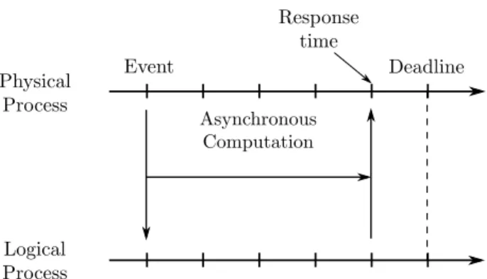
Asynchronous model
Fig. 2.5 Execution of an asynchronous model. Logical-time ≤ Physical-time. Asynchronous model is a classical representation of real-time programming [118] such as the real-time programming languages “Ada” or “C”. Applications are represented by a finite number of processes (tasks). Logical-time in the asynchronous model corresponds to the task’s processing time (see Figure 2.5). The system execution is controlled by a scheduler setting the execution dates of the application’s tasks. A task’s execution depends on the adopted scheduling policy within the Real-Time Operating
2.3 Modeling real-time systems 17
System (RTOS in short). Accordingly, in asynchronous model the logical-time is not a priori determined and may vary depending on several factor such as the platform performance or the scheduling scheme. Therefore, asynchronous model logical-time variation is constrained by real-time deadlines: logical-time must be less than or equal to physical-time. The system schedulability condition (i.e. all deadlines are met) must be indicated in the scheduling scheme of real-time operating system. A schedulability analysis also requires the analysis of the worst-case execution times.
Timed model
The principle of timed model is based on the idea that interactions between two processes can only occur at two precise moments τ and τ′. The interval between these moments (]τ,τ′[) is a fixed non-zero amount of time which corresponds to the logical duration of computation and communication between two processes (see Figure 2.6).
Fig. 2.6 Execution of a timed model. Logical-time = Physical-time.
In this context, programmers annotate their programs describing real-time systems with logical durations. The latter are an approximation of the actual computation and communication times. In this case, logical-time and physical-time are equal. Unlike the asynchronous model, since all the necessary information are known before execution, verification of some properties related to the logical temporal behaviour of the system becomes possible. For example, a scheduling validity or the system latency evaluation can be checked using a static method at compile-time.
In the timed model the program’s logical execution time is fixed, two situations may arise at the execution level:
• The program may not have finished executing while its logical execution time is exceeded. If the timed program is indeed late, a runtime exception may be thrown (an exception is usually generated).
18 Context and Problems
• The program may have completed its execution before its logical delay expiration. If the timed program finishes early, its output is delayed until the specified logical execution time has elapsed. The model annotation values should be carefully chosen in order to reduce the phase shift between the computations and output productions.
The timed model is well-suited for embedded control systems, which require timing predictability. The timed programming language Giotto [61] supports the design and implementation of embedded control systems [75], in particular, on distributed hardware. The key element in Giotto is that timed tasks are periodic and deterministic with respect to their inputs and states. The logical execution time of a Giotto task is the period of the task. For example, a 10Hz Giotto task runs logically for 100ms before its output becomes available and its input is updated for the next invocation.
Synchronous model
Fig. 2.7 Execution of a synchronous model. Logical-time = 0.
The principle of the synchronous model is similar to that of the timed model, in the sense that the two processes do not communicate between instants τ and τ′. In contrast to the timed model, the synchronous programmer assumes that any computational activity of a synchronous program including communication takes no time: logical-time in a synchronous program is always zero (see Figure 2.7). In other words, the synchrony hypothesis is satisfied as long as the system is fast enough to react to inputs coming from external environment and produces corresponding outputs before the acquisition of the next inputs. The interval ]τ,τ′[ is seen as part of the logical-time model. In order to have a detailed the system behaviour, this interval can be refined by considering intermediate instants from the logical time point of view.
2.3 Modeling real-time systems 19
In order to model the communications within multi-periodic systems, we character-ized the systems behavior using a temporal approach (a timed model). We assume that all the tasks parameters are provided by the developer.
2.3.2
Low-level languages
A large real-time systems class is implemented using low-level languages. However, the use of these languages presents several major disadvantages:
• Time-triggered communications are hard to implement. In fact, a part of the system should be scheduled manually.
• A basic mechanism for tasks communications is the “rendez-vous”, which is implemented by three primitive operations: send, receive and reply. This type of communications may lead to deadlocks such as two communicating tasks are waiting each other to resume their executions.
• A low level of abstraction makes the program correctness harder to verify (manu-ally or using automated tools).
• The use of low-level languages makes the program maintenance difficult. This is due to lack of informations differentiating parts of the program corresponding to real design constraints and parts which only correspond to implementation concerns.
Dealing with such considerations cannot be avoided. Actually, real-time systems developers tend to use programming languages with a higher-level of abstraction, where these issues are managed by the language compiler. Several languages seek to cover the entire process (from verification up to implementation). Their approach is based on translating the input program modeled with a high-level language into a low level code using automatic code generation processes. Such a strategy reduces the required time for implementation. Then, it provides a simple system description which is easier to analyse using verification tools. Finally, the compilation ensures the low-level code correctness.
2.3.3
Synchronous languages
The synchronous approach presents a high level of abstraction. This approach is based on simple and solid mathematical theories, which ease the program implementation
20 Context and Problems
and verification. Synchronous approach introduces a discrete and logical time concept defined as succession of steps (instants). Each step corresponds to the system reaction. The synchrony assumption consider that the system is fast enough to react to its environment stimulus. This practically means that the system changes occurring during a step are treated at the next step and implies that responsiveness and precision are limited by the step duration.
The synchronous execution model has been developed in order to control in deter-ministic way reactions and interactions with the external environment. Esterel [16], Lustre [56] and Signal [13] are examples of synchronous languages. In order to meet the synchrony assumption, the correct implementation of these languages requires the estimation of the worst case execution times of the program code.
Lustre
Flow or Signal is an infinite sequence of values. It describes the values taken by the
variables or expressions manipulated by a synchronous language. The sequence clock indicates the lack or the availability of a value carried by this sequence at a specific instants. The diverse features of Lustre programming language are illustrated in the following example:
n o d e NOD ( i : int ; b : b o o l ) r e t u r n s ( o : int )
var x : int ; y : int w h e n b ;
let
x = 0 - > pre ( i ); y = x w h e n b ;
o = c u r r e n t ( y );
tel
A program consists of a set of equations that are hierarchically structured using nodes. These equations defines the program output flows according to the input flows. Equations use variables of either primitive types (int, bool,...) or user-defined types. They also use a set of primitive operators (arithmetic, relational ...). In addition to those operators, there exists four temporal operators:
• "pre"(previous) operator acts as memory. It allows to refer at cycle n to the value of a flow at cycle n − 1. If X= (x1, x2, . . . , xn, . . .) is the values sequence of
the flow X, then pre(X)= (nil,x1, x2, . . . , xn−1, . . .) In this flow, the first value
is the undefined (non initialized). In addition, for any n > 1, its nth value of
2.3 Modeling real-time systems 21
• "->"(follow by) operator is used to initialize a flow. If X = (x1, x2, . . . , xn, . . .) and Y
= (y1, y2, . . . , yn, . . .) are two flows of the same type, then X -> Y= (x1, y2, . . . , yn, . . .).
This means that X -> Y is equal to Y except the first value.
• "when" operator is used to create a slower clock according to a boolean flow such as B = (true,false,...,true,...). X when B is the flow whose clock tick when B is true and its values are equal to those of X at these instants.
• "current" operator is used to get the current value which is computed at the last clock tick of the flow. If Y = X when B is a flow, then current(Y) is a flow having the same clock as B and whose value at a given clock’s tick is the value taken by X at the last clock’s tick when B was true.
i 1 2 3 4 5 . . .
b true true false false true . . .
pre(i) nil 1 2 3 4 . . .
x = 0 -> pre (i) 0 1 2 3 4 . . .
y = x when b 0 1 4 . . .
o = current(y) 0 1 1 1 4 . . .
Table 2.1 Lustre program behaviour.
The Lustre program behaviour is depicted in table 2.1. The flow value is given at clock’s tick. The node output (o) is computed according to the inputs (i,b). x and y are two local (intermediate) variables. x = 0 -> pre (i) equation sets x to 0 initially, and the subsequent x is equal to the value of i at the previous clock’s tick. y = x when b means that y is present only when b is true and it takes the value of x at this instant. Finally, the output o is defined as the current value of y when it was available.
Due to the complexity of high-performance applications and to the intrinsic combi-natorics of synchronous execution, multiple clock domains have to be considered at the application level. This is the case of a single system with multiple input/output associated with several real-time clocks. In this context, we focussing our study on modelling multi-periodic systems. In the following part, we introduce two synchronous languages dedicated to model multi-periodic systems.
Lucy-n
Synchronous languages such as Lustre [56] or Lucid Synchrone [103] define a restricted class of Kahn Process Networks which can be executed without buffers. For some
appli-22 Context and Problems
cations (real-time streaming applications), synchrony condition forces the programmer to implement manually complex buffers, which is very error-prone. In order to avoid this issue, Cohen et al. [27] generalized the synchronous approach by introducing the n-synchronous approach. This latter is based on defining a relaxed clock-equivalence. Communication between n-synchronous streams is implemented with a buffer of size n. Accordingly, quantitative information about clocks can be revealed so that the compiler can decide whether it is possible to buffer a stream into another or not.
Based on the n-synchronous approach, Mandel et al. [89] introduced Lucy-n an extension of Lustre with a build-in buffer operator. The purpose of this language is to relax synchrony constraints while ensuring determinism and execution in bounded time and memory. Lucy-n handles the communication between processes of different rates through the buffers. A clock analysis is used to determine where finite buffers must be introduced into the data flow graph. Finally, clocks and buffer sizes are computed by the compiler.
In this thesis, tasks parameters are extracted from the real-time application itself. In addition, communication between two periodic tasks are modeled using an non-flow-preserving semantics.
Prelude
Prelude [42, 41] is a real-time programming language inspired by Lustre [56]. It focuses on the real-time aspects of multi-periodic systems. Predule is an integration language that assembles local mono-periodic programs into a globally multi-periodic system.
A program consists of a set of equations, structured into nodes. Real-time constraints representing the environment requirements are specified either on nodes’ inputs/outputs (e.g. periods, deadlines) or on nodes (worst-case execution time). Equations of a node define its output flows according to its input flows. In order to manage the communication between nodes with different rates, transition operators are added to the synchronous data flow model. These operators are formally defined using strictly periodic clocks. They accelerate, decelerate, or offset flows. Therefore, they allow the definition of communication patterns provided by the user. The transition operators in Prelude allow the oversampling data sent from lower frequency tasks and under-sampling data sent from higher frequency tasks. Consequently, communications between nodes are non-flow-preserving (quasi-synchrony approach [23]).
The compiler translates a Prelude program into a set of communicating periodic tasks that respect the semantics of the original program. The tasks set is implemented as concurrent “C” threads that can be executed on a standard real-time operating
2.3 Modeling real-time systems 23
system. In case of a mono-processor platform [43], Prelude compiler implements deterministic communications between tasks without synchronization mechanisms. In order to establish these communications, the compiler ensures that the producer write before the consumer reads. In addition, it prevents a new execution of the producer to overwrite the value of its previous execution, if this latter is still required by other executions. Tasks parameters (release dates and deadlines) were adjusted in order to be scheduled on a mono-processor using Earliest Deadline First policy [85].
Our approach differs from [42, 41] in the following points: we characterize the systems behavior using a temporal approach (a timed model), in order to model the communications of multi-periodic systems. In addition, we tackle the mono-processor scheduling problem for applications modeled as non-preemptive strictly periodic tasks. Unfortunately, it has been proven [45] that the schedulability conditions for preemptive scheduling become, at best, necessary conditions for the non-preemptive case.
2.3.4
Oasis
Based on Time-Triggered Approach [77], Oasis [24, 87] is a framework dedicated to model and implement safety-critical real-time systems. An Oasis application is defined as a set of parallel communicating tasks called agents. Each agent is an autonomous running entity composed of a finite number of basic processing operations.
An Oasis application is implemented using an extension of “C” programming language, denoted by “ΨC”. This language allows the tasks specification as well as their temporal requirements and interfaces. Each task t (agent) is characterized by a real-time clock H symbolizing the physical moments at which the (input/output) data can be observed. Clocks tasks are computed according to a global (smallest) clock which include all the observable moments of the system. Each basic processing is associated with a time interval defining its earliest start time (release date) and its latest end time (deadline). This latter is also the release date of the next processing. Such specific temporal dates are called temporal synchronization points.
There are two communication mechanisms in the Oasis model. The first one is shared variables (temporal variables) defined as real-time data flows. Variables can be shared implicitly between tasks and their past values of can be read by any task that needs it. Temporal variables modifications are only made visible at synchronization points. The second mechanism for data communication is explicit message passing. Each message defines a visibility date specified by the emitting task. In fact, the message can be observed by the receiving task from this date. Moreover, messages are stored, according to their visibility, in queues that belong to the receiving task.