HAL Id: hal-01722404
https://hal.archives-ouvertes.fr/hal-01722404
Preprint submitted on 3 Mar 2018
HAL is a multi-disciplinary open access archive for the deposit and dissemination of sci-entific research documents, whether they are pub-lished or not. The documents may come from teaching and research institutions in France or abroad, or from public or private research centers.
L’archive ouverte pluridisciplinaire HAL, est destinée au dépôt et à la diffusion de documents scientifiques de niveau recherche, publiés ou non, émanant des établissements d’enseignement et de recherche français ou étrangers, des laboratoires publics ou privés.
The Competition Between Cash and Mobile Payments
in Markets with Mobile Partnerships A Monetary
Search Model Point of View
Françoise Vasselin
To cite this version:
Françoise Vasselin. The Competition Between Cash and Mobile Payments in Markets with Mobile Partnerships A Monetary Search Model Point of View. 2018. �hal-01722404�
The Competition Between Cash and Mobile Payments in Markets with
Mobile Partnerships
A Monetary Search Model Point of View
Françoise Vasselin∗
LEMMA University of Paris II December 2017
Abstract
A payment platform provides mobile money (M-money) to buyers who can also use cash to transact. An exogenous fraction of “traditional sellers” only accepts cash and creates no partnership with buyers while the remainder fraction consists of “mobile sellers” who accept M-money only and create partnerships with buyers to reduce search frictions. So, buyers without a partner must use cash and buyers with a partner must use M-money to trade. Buyers without a partner may hold cash, M-money, both monies or none while buyers with a partner always choose to hold M-money only or both monies. Hence, we obtain different equilibria where M-money always circulates, alone or in addition to cash. So, the partnership is a valuable coordination mechanism that makes M-money circulation permanent. Our model can explain why it may be useful to implement prescribed usages to trigger the adoption of a new payment instrument that aims to replace cash and why retailers implement partnerships through loyalty programs before the launching of their own M-money application. However, cash disappears only if traditional sellers have almost all disappeared.
Keywords: cash, mobile money, search theory, partnerships, investment cost, prescribed use
JEL Classification Codes : D83, E40, E50
1.
I
NTRODUCTION
Mobile devices have achieved a wide market penetration and have become ubiquitous. In 2016, there were almost as many mobile-cellular subscriptions as people in
the world (ITU [2017]). Their everyday use is based on diverse services among which
mobile payment (MP) that is “a mobile device initiated payment where the cardholder and
the merchant (and/or his/her equipment) are in the same location and communicate directly with each other using contactless radio technology, such as NFC, for data transfer” (ECP [2014]).1 According to this definition, we analyze the adoption of mobile
payments applications (MPA) at points of sales in developed countries where the NFC
technology is available.2 The MPA allow individuals to transfer bank deposits and mobile
money (M-money) that is, in a strict sense, electronic money (e-money) transferrable from
a mobile device.3 In this paper, the term M-money refers both as bank deposits and
e-money that are two kinds of book e-money that are potential substitute for cash. M-e-money is a means of payment that may contribute to reduce the use of cash that is a source of
substantial social costs (MCKINSEY [2013]). Moreover, “half of social costs are incurred
by banks and infrastructures while 46% of social costs are incurred by retailers” and
buyers incur no fraction of these costs (SCHMIEDEL et al. [2012], p6).4 So, sellers may
rationally choose to receive M-money in replacement of cash, and some of them already
refuse cash and accept M-money only; that is the case in Sweden, in China and in the
United States.5 In 2016, barely 1% of the values of all the payment in Sweden are made
using cash (SAVAGE, [2017]). Moreover, some economists think that paper money should
“be becoming technologically obsolete” (ROGOFF, 2016).
In the 1990’s, the electronic purses in the form of prepaid cards aimed to replace cash. A quarter of a century later, prepaid cards are used only by underbanked population in the US, and three projects succeeded in Asia due to a strong financial incentive to use e-money to pay for travel tickets in urban areas. By contrast, the European e-purses
1 For alternative definitions see KARNOUSKOS [2004], AU and KAUFFMAN [2008] and FED [2016].
2 The Near Field Communication (NFC) is a set of short-range wireless technologies that enables mobile devices to establish radio
communication with each other bringing them into proximity; NFC is a protocol specified by ISO/IEC 18092, it has become a standard and is supported by mobile devices of large manufacturers.
3 In a strict sense, M-money is e-money that circulates using a mobile device, it is a subset of e-money that is a monetary value
stored in an electronic device, directly or remotely (CPSS [2004]). There are three supports of e-money: a microprocessor chip embedded in a plastic card (e-money stored in e-purses such as Octopus in Hong-Kong, Suica in Japan), a remote server using computer networks (digital cash using virtual account such as PayPal) and a microprocessor chip embedded in a mobile device (M-money using an MPA (an application software that runs on mobile device) as Paylib, Starbucks’ App or Orange money).
4 “The social costs related to central banks and cash-intransit companies account for 3% and 1% respectively”, (ibid, p6). 5 See the experience of Sweetgreen in the U.S. (a popular salad quick-service restaurant) which launched a no-cash policy in 2016
(MOBILE PAYMENTS TODAY [2016]). In Sweden, you can find this kind of sign when entering a bar: “This bar accepts you for
projects failed since buyers could always use cash in all transactions and e-purses did not provide any advantages over cash. Nowadays, the MPAs allow to transfer “M-money” that competes with cash and that has some advantages over prepaid cards as it is based on the use of a mobile device. This latter allows direct interaction between consumers and merchants and supports many added services such as sending messages, ticketing, loyalty
and mobile order.6 Currently, to pay by phone, a buyer must have a prepaid or a bank
account and download an MPA. Hence, we consider that an MP platform, consisting of banks and non-banks agents provides a mobile technology that allows agents to use
M-money and benefit from added services.7 This technology is costly for buyers and we
assume that an exogenous fraction of sellers already possesses it and does not need to
invest.8 The success of the launching of M-money will depend of the definition of niche
markets in which its use is prescribed i.e. in which sellers refuse cash. Indeed, if, according to the real economy, buyers use only one means of payment to settle a transaction so, without the implementation of prescribed usages of M-money, if all sellers cannot receive it, it is not rational for buyers to hold costly M-money to trade in some transactions only, since they can use cash in all transactions. Furthermore, thanks to the high rate of smart phone equipment in developed countries, we assume that all buyers own an NFC mobile phone that supports an MPA.
The market for payment instruments is a two-sided market that presents cross-side
network externalities (ROCHET et TIROLE [2003]). So, the buyers benefit from a large
adoption of sellers and the sellers benefit from a large usage of buyers and each side of the market decides to adopt the new means of payment depending on its expectations about the adoption of the other side. This lack of coordination can be overcome by prescribed usages or/and by a mechanism such as partnerships as we formalize in this paper. Nowadays, the MP is in its launching phase and the great number of competitors does not allow us to predict exactly how this market will evolve in the coming years.
Moreover, cash remains widely used in transactions (CPMI [2016]).
However, in the US, between 2014 and 2015, the MP usage had increased from
12% to 22% for mobile phone users, and from 23% to 28% for smartphone users (FED
[2016]). Moreover, the two MPAs that are the most used in the US to pay in store are:
6 The Mobile application of retailers may also allow to pay by phone or it may be combined with an MPA offered by an MP service
provider.
7 The MPA may be provided by banks (Visa payWave, Paylib) or by non-banks: either a digital entity (Android Pay provided by
Google, PayPal) or a manufacturer (Apple Pay, Samsung Pay) or a Mobile Network Operator (Orange Cash).
8 This assumption captures the fact that M-money is compatible with the contactless payment terminals that a positive fraction of
Starbucks’ App and Dunkin’ Donuts’ App, two retailed-branded MPA (PARKS
ASSOCIATES [2016]). These latter support loyalty programs, sending of messages from
sellers and mobile orders from buyers which create a relationship between agents and that we formalize through partnerships between consumers and merchants. In the same way, Swish, the most popular MPA used in Sweden to make “more than 9 million payments a
month”, offers rewards programs (HENLEY [2016]). This situation confirms that additional
mobile services are an important driver that may encourage the M-money usage (FED
[2016]). Indeed, “to optimize the benefits of m-payment applications, these needs to be
linked to other services, such as loyalty, couponing and transport ticketing” (ECP [2013]).
These added services create a direct link between the buyers and the sellers and may influence the buyers’ portfolio choice.
M-money changes the way people pay for goods and services. Consequently, it seems important to understand how the implementation of mandatory usages of M-money in some transactions combined with mobile partnerships may affect the transactional role of cash. Could M-money replace the age-old use of cash? What is the role of partnerships in the M-money adoption process? How does the inflation rate influence the buyer’s means of payment choice, the fraction of mobile sellers required by buyers to hold M-money, and the monetary equilibria? The aim of this paper is to answer these questions in a model where the use of a medium of exchange is essential and emerges endogenously from rational decisions of buyers given the fraction of mobile sellers and the rate of partnership destruction, and where the role of the liquidity return of monies is formalized.
We propose an analytical framework to study the choice between cash and
M-money from the LAGOS-WRIGHT [2005] model to which we add some features to allow
the circulation of M-money and the creation of partnerships.At the beginning of a period,
an exogenous fraction of sellers, called “mobile sellers” can use a mobile technology to accept payment in M-money, post/send messages containing digital information that signals their location, and create partnerships with buyers. For example, in public transport, advertising posters contain a QR code that the buyers may scan with their mobile device to obtain information and that drives to the seller’s site to place a mobile order. So, mobile sellers can use the buyer’s mobile phone as a communication device to promote products, acquire and retain customers. Thus, we distinguish two types of sellers. The traditional sellers continue to accept cash, have face-to-face meetings, and search for a trading partner at each period. The mobile sellers post QR codes, only accept M-money and register the customers’ data to send them a message at each period that invites them
to visit their shop again; by this way, they create mobile partnerships that may lead to repeated meetings.
When some buyers create partnerships with mobile sellers and use M-money to transact then, in steady state, we obtain equilibria where M-money always circulates, alone or in addition to cash. So, the partnership is a valuable coordination mechanism that makes M-money circulation permanent. Furthermore, we show that when the inflation level rises, buyers require a higher exogenous fraction of mobile sellers to hold M-money and a lower fraction of mobile sellers to hold cash. And we obtain an equilibrium where M-money replaces cash if the number of traditional sellers is very low and inflation not too high. So, in our model, the replacement of cash by M-money does not only depend on the fraction of sellers capable to receive it but also on monetary policy.
Literature
New monetarist models have been used to study the competition between cash and other means of payment such as foreign currencies, capital, interest-bearing bonds and
credit.9 More related to our paper, the study of the potential replacement of cash that
competes with deposits in HE and al. [2008], with credit cards in KIM and LEE [2010],
with checks in LI [2011], and with electronic-money in LOTZ and VASSELIN [2015] allows
to determine the conditions for the coexistence of the two payment instruments and the abandon of cash. We make two different assumptions. At first, and according to the real economy, we assume that buyers use only one means of payment to settle a transaction. Consequently, with this dichotomy, and since M-money is costly for buyers, if mobile
sellers continue to accept cash, there is no equilibrium where M-money circulates.Hence,
and secondly, we assume that sellers who accept M-money refuse cash. By this way, we examine if mandatory usages of M-money are necessary or sufficient to trigger its adoption. Moreover, we model the role of a coordination mechanism through the creation of partnerships that reduce the search frictions and hence increases the liquidity return of
M-money. Furthermore, the literature in marketing and electronic commerce analyzes the
MP adoption from the generic contingency theory, the technology acceptance model, the
innovation diffusion theory and the five forces model developed by PORTER [1998]
(DAHLBERG et al. [2015]). These studies describe the actors and the factors that influence
9 See NOSAL and ROCHETEAU (2011), LI (2011), ROJAS BREU (2013), GU et al. (2015), LIU (2016) and LOTZ and ZHANG (2016)
the MP market, identify the relevant stakeholders, and the main economic theories applicable. Nevertheless, these reviews remain descriptive and don’t formalize the competition between M-money and traditional means of payment while there is a need to compare them. Moreover, none of these last studies consider the role of the fraction of sellers accepting MP while this fraction determines the extent of search frictions in the market. In addition, they do not study the role of a coordination device even if they often mention the role of loyalty programs that create a direct link between consumers and merchants. Consequently, it seems useful to formalize the role of partnerships in the choice of the buyer between cash and M-money.
To allow M-money to compete with cash, the transactions settled in cash must have
drawbacks. HE and al. [2008], LOTZ and VASSELIN [2015] introduce a risk of theft, KIM
and LEE [2010] consider a disutility cost, NOSAL and ROCHETEAU [2011, Ch5] consider a
portability cost and LI [2011] considers forgone interest incomes. In our model, we
consider that an exogenous fraction of sellers can use a mobile technology to receive
M-money which allows them to reduce their management cost of cash.10 In the literature,
most studies consider that either buyers or sellers pay a fixed record keeping cost to register their trading histories and their identity. We consider that buyers pay a fixed cost to the MP platform for using M-money and that some sellers can use a mobile technology that records M-money transfers only. Under the proportional bargaining solution, the cost paid by the buyer affects the terms of trade and it is shared between the partners. In addition, the creation of mobile partnerships requires repeated meetings between
consumers and merchants during the trading period. AIYAGARI and WILLIAMSON [2000],
CORBAE and RITTER [2004], NOSAL and ROCHETEAU [2011, Ch8] allow individuals to
create long-term partnerships using credit. We also allow agents to enter in repeated interactions but mobile partnerships differ from credit arrangements since buyers meet sellers in the decentralized market only, and not in the centralized market. So, in this
economy, buyers do not use credit to settle transactions.11 Finally, mobile partnerships
may end through an exogenous shock as in CORBAE and RITTER [2004] and in NOSAL and
ROCHETEAU [2011]. We assume that this shock destroys the customer database and
prevents mobile sellers to interact with their partner at the beginning of the following
10 Banks and merchants directly incur most of the operational cost of cash (MCKINSEY [2013], p5). Moreover, the cofounders of
Sweetgreen justify the choice of the MP application in the following way: “It costs money to handle cash, specifically the transfer
of it via armored trucks (…) and employees conduct more transactions every hour, some 5-to-15 percent more, if they don’t have to handle cash” (MOBILE PAYMENTS TODAY [2016]).
period. Symmetrically, the seller may be hit by a relocation shock and the buyer ignores its new location. This assumption guarantees a permanent flow of search activity.
However, by difference to NOSAL and ROCHETEAU [2011, Ch8], the partnership
destruction occurs after the buyers’ portfolio choice and then, the partnerships duration affects the liquidity return of each money.
So, in our model, we formalize the role of mobile partnerships that constitute a coordination mechanism allowing the agents to internalize the network externalities associated with the adoption of a new means of payment that aims to replace cash, and the role of mandatory usages of a means of payment. The paper is organized as follows. Section 2 presents the environment. Section 3 describes the value functions of agents in the markets. Section 4 defines the terms of trade. Section 5 analyzes the portfolio choice of unattached buyers. In section 6, we analyze the portfolio choice of buyers attached to a mobile seller. In section 7, we study monetary equilibria. Section 8 concludes.
2.
E
NVIRONMENT
Time is discrete and continues forever. Agents (buyers and sellers) live infinitely and successively visit two markets. In the decentralized market (DM) anonymous buyers and sellers, specialized in consumption and in production, are matched randomly and trade
bilaterally. Sellers can produce an output in quantity ∈ ℝ but do not consume, while
buyers want to consume but cannot produce. Then, agents enter a frictionless centralized
market (CM). In the CM, all individuals can consume or produce a general good ∈ ℝ
by supplying labor ℎ and adjust their portfolios. The DM and CM goods are non-storable
so, they cannot serve as a means of payment. The utility functions of buyers ( ) and
sellers ( ) for the entire period, assumed separable between the two sub-periods are
described as follows:
, , ℎ = + − ℎ
, , ℎ = − + − ℎ
The agents' utility function is linear in the CM with their labor hours, and the utility
and the cost functions have the following properties: > 0, < 0, > 0,
> 0, 0 = 0 = 0 = 0, and 0 = +∞. The optimal level of output that
maximizes the agents' trade surplus, − , is noted ∗ and satisfies ∗ = ′ ∗ .
In this economy, each buyer enters the DM with a portfolio , consisting of nominal units of cash and/or nominal units of book money transferrable by phone i.e. M-money. The value of money ( ) changes over time so, the nominal monetary units
and are valued at =
!, being the price of money in terms of the general good at
time ". Thus, a portfolio , has a real value # = + ≡ % + &. The aggregate stock
of money in the economy ' can be held in the form of cash and/or in the form of
M-money and it can increase or decrease in each period at the constant gross rate ( ≡)!*)! .
Money is injected or withdrawn from the economy through lump-sum transfers + from the
government in the CM. Finally, we focus on stationary equilibrium where the real value
of the money supply is constant over time: ' = ,' ,, and where: ( = -!
-!*
measures the inflation rate.
Furthermore, an MP platform consisting in banks and/or non-banks agents (such as mobile network operators, digital entity or manufacturers) provides M-money to buyers and we assume that it makes zero profit. Moreover, at the beginning of the DM, an
exogenous fraction . > 0 of sellers uses a mobile technology that allows to receive
M-money and create a customer database. These sellers are referred to as mobile sellers who refuse cash and accept M-money only. Moreover, in the CM, the buyers choose their portfolio composition, they may choose cash, M-money or both. If they choose to hold M-money, they may open a bank account and download an MPA. Then, the MP platform accepts cash and transfers an equivalent amount of M-money units in the buyer’s bank account. Then, the buyer can transfer M-money to mobile sellers using the MPA. During a meeting between a buyer and a mobile seller, agents create a partnership that can be maintained in the following DM and so, agents begin the next DM attached to a trading
partner into a mobile partnership. The remaining fraction of sellers 1 − . consists of
traditional sellers who accept cash only, cannot create a partnership and seek for a trading partner at each period. So, in the DM, buyers and sellers enter either attached or unattached to a DM trading partner. Unattached buyers and sellers participate to a random
matching process and meet each other with probability / ∈ 0,1 . Finally, since there are
two types of sellers, unattached buyers may find either a traditional seller with probability / 1 − . or a mobile seller with probability /..
In the DM, agents bargain a pair ( , 0) where the buyer acquires a quantity of
DM output in exchange for a payment 0 (dollars) to the seller. In a traditional match,
quantity 1 ≡ % of goods in exchange for 01≡ 0 % units of cash and agents will not meet again in the future DM. In a mobile match, two events occur. At the beginning of the DM, mobile sellers post advertising with QR codes containing digital information such
as their location. The mobile sellers only accept M-money (&), and agents bargain a pair
( 2, 02). The mobile seller produces the quantity 2 ≡ & in exchange for 02 ≡ 0 &
units of M-money. Moreover, during a mobile match, agents create a mobile partnership
that is only active in the DM so, it does not exist in the CM.12 Since agents are not attached
for the entire period, they cannot negotiate debt contracts that buyers would repay in the CM, before the next period.
Furthermore, at the end of each period, a fraction of mobile partnerships is
exogenously destroyed with probability 4 ∈ 0,1 and both agents begin the following
period without a partner. At the beginning of the DM, if the partnership is not destroyed,
the fraction 1 − 4 of agents who remain attached find each other with probability one,
otherwise, they participate to a random matching process as unattached agents. Since the fraction of sellers and buyers is equal, the fraction of unattached buyers and sellers is also
equal. Moreover, since 4 ∈ 0,1 and / ∈ 0,1 then, if there exists a positive fraction of
mobile partnerships at a period ", in steady state, there exists a positive fraction of mobile
partnerships at each period. Finally, in the CM the buyers pay a fixed usage cost Ω > 0 to
the MP platform if they used M-money to transact in the DM and the platform has a commitment technology: it must redeem M-money in cash to M-money holders (buyers and sellers) when they enter the CM. Then, in the CM, all agents can exchange cash for
general goods at price and readjust their portfolio. The timing of events is represented
in the figure 1. Discount factor across period: 6 Day (DM) Night (CM) 6 + 7 An exogenous fraction . of mobile sellers post QR codes
Unattached buyers find a traditional seller with probability / 1 − . or
a mobile seller with probability /. Traditional sellers produce 1for 01 Mobile sellers produce 2 for 02
Buyers pay the usage cost of M-money 8 > 0 Buyers choose their portfolio (% ≥ 0, & ≥ 0) A fraction 4 ∈ 0,1 of mobile partnerships ends
Presence of a mobile payment platform
FIGURE 1. - Timing of events
12 The agents who formed a mobile partnership in the DM have not the possibility to meet each other once again in the CM and
then, credit is not feasible. No mobile seller knows the precise location of buyers after the DM. They can only invite them to visit their shop again at the beginning of a new period by sending a new message.
3.
T
HE CENTRALIZED AND THE DECENTRALIZED MARKETS
We begin the analysis by the centralized market (CM) then, we analyze the decentralized market (DM). The buyers leave the DM either “unattached” or “attached” to a trading partner for the next DM through a mobile partnership and enter the CM.
3.1. Value functions of buyers unattached into a mobile partnership
In this section, we describe the value functions of agents who are without a partner, and the value they obtain in a traditional and in a mobile match.
The expected lifetime utility of an unattached buyer (index “ ”), i.e. a buyer who is
not attached to a mobile seller, who enters the CM with the wealth :, satisfies:
;< : = max@,A,1B,2BCDE − ℎ + F< % , & G
H. ". + + = ℎ + : + +
, + ′ = % + &
where F< % , & is the value function of an unattached buyer at the beginning of the next
period. From the second equation that is the buyer’s budget constraint, an unattached
buyer finances his consumption in the CM ( ) and his next period portfolio , ′ from
his labor (ℎ), his wealth (:) and the lump sum transfers from the government (+). From
the previous problem, the value function of an unattached buyer who enters the CM is given by:
;< : = : + + + max
1B,2BCDE−( % + & + F< % , & G (1)
From (1), the buyer enters the CM with the wealth :, receives a transfer + and accumulates
( % + & units of monetary assets for the next period. Notice that the buyer’s portfolio choice is independent of his wealth when entering the CM. Moreover, the DM value
function of an unattached buyer F< %, & depends on the two meetings he may have and
is written:
In the DM, with probability / 1 − . an unattached buyer meets a traditional seller and
the value of this traditional match (index “+”) is FJ %, & , with probability /. he meets
a mobile seller and the value of this mobile match (index “'”) is FK %, & . Finally, with
probability 1 − / , the buyer meets no seller, remains unattached and his continuation
value is ;< %, & .
Moreover, in a traditional match, the DM value function of an unattached buyer
with a portfolio # = % + & consisting of % units of cash and & units of M-money is:
FJ %, & = 1 + ;< # − 01 . The buyer purchases 1 units of goods in exchange for
01 units of cash and enters the CM with # − 01 units of monetary assets. From the linearity
of ;< we get:
FJ %, & = 1 − 01+ #+;< 0 (3)
Furthermore, in a mobile match, the buyer transfers M-money and obtains the value:
FK %, & = 2 +;K # − 02+ Ω and from the linearity of ;K we get:
FK %, & = L 2 − 02− ΩM+# + ;K 0 (4)
From (4), in a mobile match, the buyer purchases the quantity 2 for 02 units of M-money
and pays the cost Ω in the CM and then, agents create a mobile partnership for the next
DM.
3.2. Value functions of buyers attached into a mobile partnership
At the beginning of the CM, the value function of a buyer attached to a mobile
seller and who enters the CM with the wealth : is given by:
;K : = max@,A,1B,2BCDE − ℎ + N4F< % , & + 1 − 4 FK % , & OG
H. ". + + + Ω = ℎ + : + +
, + = % + &
The second equation indicates that a buyer attached to a mobile seller finances his
M-money from his labor (ℎ), his wealth (:) and the transfers (+). From the previous problem, the CM value function of a buyer attached to a mobile seller is:
;K : = : + + −Ω + max
1B,2BCDP−( % + & + L4F< % , & + 1 − 4 FK % , & MQ (5)
An attached buyer who enters the CM with the wealth :, receives the transfers +, pays
the cost Ω if he used M-money in DM, accumulates ( % + & units of monetary assets,
and if the partnership ends with probability 4, his DM value function is F< % , & or if
the partnership continues with probability (1 − 4), his DM value function is FK % , & .
4.
T
HE BARGAINING SOLUTION AND THE TERMS OF TRADE
We now describe the determination of the terms of trade in a bilateral match in the
DM between a buyer who enters the market with the portfolio # = %, & and a seller
without money. To give the buyers incentives to incur the cost Ω > 0, we adopt the
proportional bargaining solution of KALAI [1977] according to which the buyer receives
a constant share R ∈ 0,1M of the total match surplus and the seller gets the remaining
fraction: 1 − R > 0.
4.1. The determination of the terms of trade when cash is used to
settle transactions
If a buyer uses cash to transact in a match, agents bargain a pair 1, 01 . The buyer’s and
the seller’s surplus are 1 + ; # − 01 − ; # and − 1 + ; 01 − ; 0 ,
respectively. From the linearity of ;, the buyer’s surplus is S1 = 1 − 01, the seller’s
surplus is S1 = 01− 1 , and the total math surplus with cash is S 1 = 1 − 1 .
Finally, the pair 1, 01 results from the following program:
1, 01 = maxTUV1P 1 − 01Q
H. ". 1 − 01 =,XWW L01− 1 M
According to the previous problem, the buyer maximizes his utility of consuming the
quantity 1 net of the transfer of 01 units of cash; subject to the constraints that his trading
surplus is equal to R 1 − R⁄ times the seller’s trading surplus and he cannot transfer to
the seller more money than he holds (01 ≤ %). From the second equation, the terms of
trade in a traditional match are defined as follows:
01 = [ 1 ≡ 1 − R 1 + R 1 (6)
The payment to the seller [ 1 is a continuous function so, there exists a solution for the
buyer’s choice of money holdings. From (6), the buyer spends all his units of cash % to
purchase 1 units of output. Substituting the terms of trade from (6) into the previous
program, the buyer’s problem can be simplified to:
\ 1 = max]U RP 1 − 1 Q
H. ". [ 1 ≤ %
Consequently, the quantity of DM goods 1 depends on the real value of cash transferred
in a match and is given by:
1 = ^ [
X, % _` % < [ ∗
∗ _` % ≥ [ ∗
4.2. The determination of the terms of trade when M-money is used to
settle transactions
In a mobile match, the buyer’s and the seller’s surplus are written 2 +
; # − 02− Ω − ; # and − 2 + ; 02 − ; 0 , respectively. From the
linearity of ;, the buyer’s surplus with M-money is written: S2 = 2 − 02− Ω and
the seller’s surplus is S2= 02− 2 . Consequently, the net total match surplus with
M-money is written: Sa 2 = S 2 − Ω and it is measured by the difference between the
total match surplus with M-money S 2 = 2 − 2 and the buyer’s M-money
Lemma 1. The buyer’s M-money usage cost Ω > 0 is a transaction cost that reduces the
total match surplus with M-money S 2 leading to a lower match surplus: Sa 2 =
S 2 − Ω. The use of M-money reduces the size of the trading surplus.
Finally, the pair 2, 02 results from the following program:
2, 02 = maxT
bV2P 2 − 02− ΩQ
H. ". 2 − 02− Ω =,XWW L02− 2 M
02 ≤ &
According to the previous problem, the buyer maximizes his utility of consuming
the quantity 2 net of 02 units of M-money and the cost Ω ; subject to the constraints that
his trading surplus is equal to R 1 − R⁄ times the seller’s trading surplus and he cannot
transfer to the seller more M-money than he holds. From the second equation, the terms of trade in a mobile match are given by:
02= [ 2 ≡ 1 − R L 2 − ΩM + R 2 (7)
Equation (7) may be rewritten: [ 2 = 1 − R 2 + R 2 − 1 − R Ω. So, if the
buyer uses M-money, his payment [ 2 decreases with the term 1 − R Ω that is the
seller’s share of the buyer’s M-money usage cost. This corresponds to a commercial advantage or a subsidy from sellers. From (7), the buyer spends all his units of M-money
& to purchase 2 units of goods. Substituting the terms of trade from (7) into the previous
program, the buyer’s problem becomes:
\ 2 = &#]b RP 2 − 2 − ΩQ
H. ". 1 − R L 2 − ΩM + R 2 ≤ &
Consequently, the quantity of DM goods 2 depends on the real value of M-money
transferred in the match and is given by:
2 = ^ [
X, & _` & < [ ∗
Lemma 2. The buyer’s M-money payment to the seller is reduced from the amount
1 − R Ω and then, the seller produces, and the buyer consumes a higher quantity of goods
in exchange for M-money than for cash 2 > 1. If Ω = 0, agents trade the same quantities in all matches: 2 = 1.
Furthermore, an increase in the buyer’s bargaining power R decreases the share of the
buyer’s M-money cost incurred by mobile sellers. If the buyer makes a take-it-or-leave-it
offer, the seller receives zero surplus. From (7), when R = 1 , 02 = 2 and the buyer’s
money transfer covers exactly the seller’s production cost. So, if R = 1, the seller’s
subsidy is not feasible.13
5.
T
HE PORTFOLIO CHOICE OF UNATTACHED BUYERS
In this section, we describe the choice of money holdings of an unattached buyer when he uses cash in a traditional match and M-money in a mobile match.
5.1. The objective function of unattached buyers and the liquidity
return of monies
Before entering the DM, an unattached buyer chooses his portfolio composition from his CM value function (1). By replacing the terms of trade (6) and (7) into (3) and (4) the DM value functions of a buyer in a traditional and in a mobile match are written:
\ FJ %, & = RP 1 − 1 Q + #+;< 0
FK %, & = RP 2 − 2 − ΩQ+# + ;K 0 (8)
By inserting the previous equations into F< %, & defined in (2), the DM value function of
an unattached buyer who enters the DM with the portfolio # = % + & is written:
F< %, & = RP/ 1 − . L 1 − 1 M + /. L 2 − 2 − ΩM Q + c d e.f,Xe. f)g D
hg Di (9)
13 This confirms the results of J. ROBINSON [1969] who identified that a positive market power of sellers is a necessary condition
According to (9), with probability / 1 − . an unattached buyer meets a
traditional seller and obtains the fraction R of the surplus in a traditional match and with
probability /. he meets a mobile seller and obtains the fraction R of the surplus in a
mobile match. The last three terms result from the linearity of ;< and ;K and correspond
to the continuation value in the CM when no transaction occurred. Substituting F< from
(9) into (1), we obtain the objective function of an unattached buyer from which he chooses his money holdings for the next period (Appendix 1):
Γ< %, & = max
1,2CDE−_ % + & + RP/ 1 − . L 1 − 1 M + /.L 2 − 2 − ΩMQG (10)
From (10), an unattached buyer chooses the amount of cash (% ≥ 0) and M-money
(& ≥ 0) so that he maximizes his share R of the expected match surplus in the DM net of
the holding cost _ of each unit of money.14 The function (10) is strictly concave which
guarantees that a solution exists. The quantities of DM goods 1< and 2<, respectively traded for cash in a traditional match and for M-money in a mobile match by unattached buyers (exponent “ ”) in equilibrium, result from the first order conditions associated to (10) and satisfy (Appendix 2):
−_ + / 1 − . ,XW kWNkBl]Bl]UhmXnBl]UhmO
Uhm WnBl]Uhm≤ 0 (11)
−_ + /. WNkBl]bhmXnBl]bhmO
,XW kBl]bhm WnBl]bhm≤ 0 (12)
Condition (11) is satisfied with an equality if % > 0 and condition (12) if & > 0. From
(11-12), the buyer brings positive units of cash and/or M-money in the DM up to the point
where he equalizes the holding cost _ of a marginal unit of each type of money with its
liquidity return o . ≡ WNkB . XnB . O
,XW kB . WnB . in the match. The liquidity return measures the
expected marginal increase in the trade surplus that results from the possibility to exchange one supplementary unit of each money against goods. From (11), the buyer
chooses to bring cash in the DM if the cost _ of holding an additional unit of cash is equal
to its liquidity return if he meets a traditional seller. From (12), the buyer chooses to carry
M-money if the cost _ of holding an additional unit of M-money is equal to its liquidity
return if he meets a mobile seller. So, the liquidity return of each money is affected by the
14 Where the interest rate _ satisfies: _ =pqr
r . Notice that a buyer can only purchase the optimal quantity of output ∗ at the Friedman rule, when _ = 0. We consider in what follows that _ > 0, hence the quantity traded in the DM is such that < ∗.
fraction of each type of sellers, while it is independent of buyer’s M-money cost Ω which does not affect the marginal surplus but only the surplus and the terms of trade.
5.2. Valuation of monies by unattached buyers
In this section, we describe the valuation of monies by unattached buyers who may use cash in a traditional match or M-money in a mobile match depending on the type of
seller they meet. We focus our intention on the exogenous fraction . > 0 of mobile
sellers that allows attached buyers to use M-money, and on the level of the interest rate _ > 0 that, respectively, capture the role of network externalities and inflation in the choice of a means of payment by consumers.
The quantities 1< and 2< traded by an unattached buyer in equilibrium are solution
to (11-12). After rearrangements, (11) becomes:
1< 1< =
R _ + / 1 − . R/ 1 − . − _ 1 − R
The right side of this equation increases with . and _ then, a rise in . or _ decreases 1<
and hence %. Consequently, the buyer’s choice of cash is decreasing in . and _. Indeed,
if it is more likely to find a mobile seller, thus cash is needed in a smaller fraction of transactions and the buyers optimally hold less cash and more M-money. Similarly, if the
holding cost of cash _ increases, buyers rationally choose to hold less cash. Consequently,
there is a threshold value for ., or for _, from which unattached buyers don’t hold cash
anymore. That is the case when the denominator is equal to zero or when: .sss1< =LeWX ,XW tM
eW
or u̅1< = eW ,X.
,XW . Hence, unattached buyers value cash if . < .sss1< or equivalently if _ <
u̅1<. Moreover, the quantity 2< is solution to (12), and after rearrangements (12) becomes:
2< 2
< =R/. − _ 1 − RR _ + /.
The right side of this equation decreases with . and increases with _. So, a rise in
. increases 2< and hence & and a rise in _ decreases 2< and &. By equalizing the
denominator to zero, we obtain the threshold values for . and _ and then, unattached
buyers value M-money if . > .sss2< = ,XW t
eW or equivalently if _ < u̅2< = eW.
,XW. Furthermore,
the critical values for the fraction . of mobile sellers, .sss1< and .sss2<, depend on the interest
M-money. In figure 2, we represent the evolution of the threshold values .sss1< and .sss2<,
depending on _. When .sss1< = 0 ⟹ _ = eW
,XW≡ _1,2< , and .sss2< = 1 ⟹ _ = eW
,XW≡ _1,2< .
Moreover, the two curves intersect for .sss1< = .sss2< ≡ .sss~< = ½. i.e. when buyers are
indifferent between both monies or when: _ = eW
z ,XW = {U,b h | ≡ _~<. ., .sss1<, .sss2< 1 2 1 &<≥ 0 .sss2< = 1−R _/R &<≥ 0 %<= 0 &<= 0 .sss~<= ½ %<≥ 0 %<= 0 &<= 0 .sss1<=LeWX ,XW tMeW %<≥ 0 0 _~<=_%,&2 _1,2< = 1−R/R _
FIGURE 2. – Valuation of cash and M-money by unattached buyers depending on _
In figure 2, the threshold value .sss1< below which unattached buyers value cash is
decreasing in _. Indeed, when the holding cost of cash increases, buyers require higher
probability to use it to transact i.e. a lower fraction of mobile sellers. Similarly, the critical
value .sss2< above which they value M-money is increasing in _. Indeed, when the holding
cost of M-money rises, buyers require a higher probability to use it i.e. a larger fraction
of mobile sellers. Finally, cash is valued when . < .sss1< (%< ≥ 0) and M-money is valued
when . > .sss2< (&< ≥ 0).
Furthermore, when the interest rate is low and precisely when _ < _~< (region 1 in
figure 2), we distinguish three different regions where either both monies (% ≥ 0, & ≥ 0),
or only M-money (& ≥ 0, % = 0 , or only cash (% ≥ 0, & = 0) are valued. When _ ≥ _~<
(region 2 in figure 2), we also distinguish three regions, but unattached buyers don’t value
both monies at the same time, and either cash or M-money is valued, or no money is valued. Hence, when the inflation is low, both monies may circulate but a higher inflation forces buyers to hold only one or other of these monies since their holding cost is larger. In addition, higher inflation is, the more buyers require a large fraction of mobile sellers to hold M-money. Consequently, we distinguish two situations, low and high inflation.
Lemma 3. When buyers are without a partner, there is a critical value .sss1< for the fraction
. of mobile sellers such that if . ≥ .sss1<, cash is no longer valued, and there is a critical
value .sss2< for the fraction . of mobile sellers such that if . ≤ .sss2<, M-money is not valued. A rise in the interest rate _ increases .sss2< and decreases .sss1< so, when inflation increases, buyers require a lower fraction . to hold cash and a higher fraction . to hold M-money.
5.3. The quantities traded and the portfolio choice of unattached
buyers
In this section, we analyze the quantities traded by unattached buyers that determine their portfolio composition in an economy with low inflation and then, with high inflation.
1) Quantities traded by unattached buyers in an economy with low inflation
From figure 2, when inflation is low (_ < _~<), the quantities traded by unattached buyers
for cash and M-money depend on the fraction . of mobile sellers as in figure 3.
1<, 2< 1< 2< 1<,D= 2<,, ~< ~ • € • 0 .sss2< .sss~<= ½ .sss1< 1 .
FIGURE 3. – Quantities traded by unattached buyers in an economy with low inflation
Let 1<,D be the solution to (11) when . = 0 and 2<,, the solution to (12) when . = 1, /ol 1<,Dm = /o 2<,, and hence 1<,D = 2<,,. Then, the quantities exchanged for cash are strictly decreasing in . from 1<,D until .sss1< from which cash is no longer valued.
Similarly, the quantities exchanged for M-money are strictly increasing in . above .sss2<
where M-money is valued and until 2<,, when . = 1. The curves intersect for . = .sss~<
,
z/ol 1<,,/zm = ,
z/ol 2<,,/zm, .sss1< = .sss<2 and 1<,,/z= 2<,,/z = ~<. Finally, we obtain four
intervals for the fraction . of mobile sellers: “~”, “•”, “€” and “•” that influence the
buyers’ portfolio choice. Subsequently, to study the competition between cash and M-money and determine the conditions for M-M-money adoption, we study the buyer’s
portfolio choice for _ ∈ L0, _~< and for different fraction . ∈ L0,1M when cash is used in
traditional match and M-money in mobile match. We consider different buyers’ expectations of the number of mobile sellers in the economy that determine different portfolio choices from (11-12).
If the exogenous fraction of mobile sellers is such that . ∈ L0, .sss2<M (interval ~)
only cash is valued so 2<,ƒ= 0 and the quantity traded 1<,ƒ> 0 is solution to (11), where
the exponent “~” refers to . ∈ L0, .sss2<M. If . ∈ .sss2<, ½ (interval •), they value both monies and from (11-12), there exists a quantity 1<,„ > 0 and a quantity 2<,„ > 0 such
that: / 1 − . ol 1<,„m = /.ol 2<,„m. Since 1 − . > ., both monies are valued if
ol 1<,„m < o 2<,„ ⟺ 1<,„ > 2<,„ (figure 3). Moreover, if . ∈ L½, .sss1< (interval €), from (11-12), there exists quantities 1<† > 0 and 2<,† > 0 such that / 1 − . ol 1<,†m = /.ol 2<,†m. Since, 1 − . < ., both monies are valued such that ol 2<,†m < o 1<,†
⟺ 1<,† < 2<,†(figure 3). Finally, if . ∈ N.sss1<, 1O, (interval •), only M-money is valued and from (12): 2<,‡ > 0.
2) Quantities traded by unattached buyers in an economy with high inflation
From figure 2, when inflation is high (_ ≥ _~< in region 2, the quantities traded for
cash and M-money depend on the fraction . of mobile sellers in the economy as in figure
4, and there is no coexistence of the two monies. 1<, 2< 1< 2< 1<,D = 2<,, ˆ ‰ 0 .sss1< .sss2< 1 .
If the exogenous fraction of mobile sellers is such that: . ∈ L0, .sss1< , (interval ˆ),
only cash is valued. So, 2<,Š = 0 and the quantity 1<,Š > 0 is solution to (11). If . ∈
.
sss2<, 1M, (interval ‰), only M-money is valued. So, 1<,‹ = 0 , and the quantity
2<,‹ > 0
is solution to (12).
3) Decisions of unattached buyers
In figure 5a, we represent the quantities traded by unattached buyers depending on
the fraction . of mobile sellers and inflation. In figure 5b, we obtain four possible
arrangements from the portfolio choice of buyers unattached into a mobile partnership (exponent " "). Firstly, when . > .sss2<, M-money is valued and if . < .sss1< unattached
buyers hold both cash (%) and M-money (&) to trade with a traditional or a mobile seller (letters
" %&& <") while if . ≥ .sss 1
<, they hold M-money only to trade with mobile sellers (letter
"&<"). Secondly, when . ≤ .sss2<, unattached buyers do not value M-money and if . < .sss1<,
they hold cash only to trade with a traditional seller ((letter "%<"). Finally, if . ≥ .sss1< no money is valued then, no money circulates (symbol " 0,0 <").
., .sss1<, .sss2< ., .sss1<, .sss2< 1 .sss2< 1 .sss 2 < 2<> 0 1<= 0 2<> 0 1<= 0 2<> 1< &< 1<= 0 .sss~< .sss~< %&&< 0,0< 1<> 2< 2<= 0 %< 1<> 0 2<= 0 2<= 0 1<> 0 .sss1< .sss1< 0 _~< _1,2< _ 0 _~< _1,2< _
Figure 5a. Figure 5b.
FIGURE 5. – Decisions of unattached buyers for different values of . and _
6.
T
HE PORTFOLIO CHOICE OF ATTACHED BUYERS
In this section, we describe the choice of money holdings of an attached buyer who already used M-money in the previous period and who chooses his next period portfolio depending on the rate of partnership destruction and given the exogenous fraction of mobile sellers.
6.1. The objective function of attached buyers and the liquidity return
of monies
A buyer attached to a mobile seller chooses his portfolio composition from the
maximization of his CM value function (5). By substituting in (5) FK %, & and F< %, &
by their expression from (8) and (9) we obtain the objective function of an attached buyer
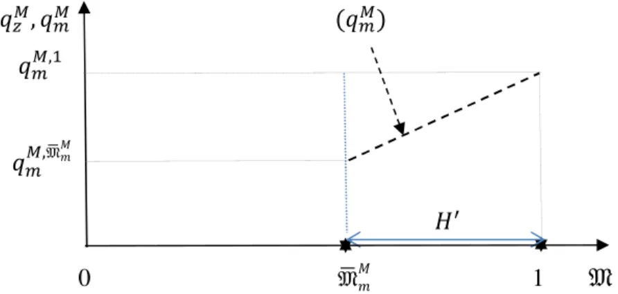
ΓK %, & (Appendix 3): ΓK %, & = max 1,2CDŽ−_ % + & + R •λ ‘ / 1 − . L 1 − 1 M +/. ’ 2 − 2 −Ω “ ” + 1 − λ • 2 − 2 −Ω –—˜ (13)
From equation (13), the buyer chooses his real balances (% ≥ 0) and his M-money (& ≥
0) so that he maximizes his share R of the expected trade surplus in the DM net of the
holding cost _ of each monetary asset if he expects that the partnership ends with
probability λ and if he expects that the partnership continues with probability 1 − λ .
Indeed, a buyer attached to a mobile seller may meet a traditional seller if the partnership
ends and trade the quantity 1K in exchange for cash, or he may meet his partner if the
partnership continues or another mobile seller if the partnership ends and trade the
quantity 2K. The quantities of DM goods 1K and 2K, respectively traded for cash in a
traditional match and for M-money in a mobile match by a buyer attached into a mobile
partnership (exponent “'”) in equilibrium, result from the first order conditions
associated to (13) and are:
−_ + λ/ 1 − . R kBl]U)mXnBl]U)m
,XW kBl]U)m WnBl]U)m≤ 0 (14)
−_ + L1 − λ 1 − /. MR kBl]b)mXnBl]b)m
,XW kBl]b)m WnBl]b)m≤ 0 (15)
Condition (14) is satisfied with an equality if % > 0 and condition (15) if & > 0. From
(14), a buyer attached to a mobile seller chooses to hold cash if the cost _ of holding an
additional unit of cash is equal to its liquidity return if the partnership ends and if he meets
a traditional seller. From (15), the buyer chooses to hold M-money if the cost _ of keeping
an additional unit of M-money is equal to its liquidity return if he meets a mobile seller when the partnership continues or when a new partnership is created after the destruction
M-money in a mobile match. So, the liquidity return of each type of M-money now depends
both on the fraction of each type of sellers and the probability λ of partnership destruction.
6.2. Valuation of monies by attached buyers
In this section, we describe the valuation of monies by an attached buyer who used M-money in a mobile match and who created a partnership with a mobile seller in the previous period. His next period portfolio choice now depends on the rate of partnership destruction. Indeed, if the partnership ends, he may use cash in a traditional match or M-money with a new mobile seller, and if the partnership continues, he uses M-M-money with
his partner. The quantities 1K > 0 and 2K > 0 traded by buyers attached into a mobile
partnership are solution to (14-15). After rearrangements (14) becomes:
1K 1K =
R _ + λ / 1 − . Rλ / 1 − . − _ 1 − R
The right side of this equation increases with _ and . and decreases with 4 so, a rise in _
or in . decreases 1K and hence %, and a rise in λ increases 1K and %. Indeed, a rise in 4
increases the probability to use cash to transact in the next DM, therefore the demand for
cash increases. So, attached buyers value cash if _ < u̅1K ≡ W™ e ,X.
,XW or equivalently if . <
.
sss1K ≡ W™ eXt ,XW
W™ e , and .sss1K < .sss1<. Moreover, after rearrangements (15) becomes: 2K
2
K =RL1 − λ 1 − /. M − _ 1 − RRL_ + 1 − λ 1 − /. M
From the previous equality, attached buyers value M-money if _ < u̅2K ≡WL,X™ ,Xe. M
,XW or
if . > .sss2K ≡t ,XW XW ,X™
W™ e and .sss2K < .sss2<.
Lemma 5. ∀4 < 1, .sss1< > .sss1K and .sss2< > .sss2K. So, attached buyers don’t value cash and value M-money for a lower fraction of mobile sellers than unattached buyers.
Moreover, .sss2K = 0 if _ =W ,X™
,XW ≡ û2K, .sss1K = 0 if _ = W™ e
,XW ≡ _1K, .sss2K = 1 if _ = WL,X™ ,Xe M
,XW ≡ _2K, .sss1K = 1 if _ = 0, _1K < _2K ∀λ < 1, and the two curves intersect for _ =
WL,X™ ,Xe M
z ,XW = _~K > _~<. Moreover, from (14-15) attached buyers are indifferent between
cash or M-money if λ/ 1 − . o 1K = L1 − λ 1 − /. Mo 2K or if . =™eX ,X™
.
sss~K < .sss~<. Furthermore, _K1 > _~K if 1 − λ < λ/ .15 The figure 6a. and 6b. represent .sss 1 K
and .sss2K depending on _ when 1 − λ < λ/ and when 1 − λ ≥ λ/ respectively.
., .sss1K, .sss2K 1 2 3 1 &K≥ 0 .sss2K =t ,XW XW ,X•W• e %K= 0 &K≥ 0 &K= 0 .sss~K=™eX ,X™z™e %K ≥ 0 %K= 0
&K= 0 .sss1K=W• eXt ,XWW• e %K ≥ 0
0 û2K _~K _K1 _1,2< _2K _
FIGURE 6a. – Valuation of cash and M-money by attached buyers when 1 − λ < λ/
.,.sss1K, .sss2K 1 2 3 1 .sss2K=t ,XW XW ,X•W• e &K≥ 0 %K= 0 &K ≥ 0 &K= 0 %K≥ 0 %K = 0 .sss 1 K =W• eXt ,XW W• e 0 _1K _~K û2K _2K _
FIGURE 6b. – Valuation of cash and M-money by attached buyers when 1 − λ ≥ λ/
In figure 6b., the curves intersect in the negative orthant and we do not analyze this
situation since . > 0. Moreover, in figures 6a. and 6b., we distinguish three inflation
levels, very low (_ < û2K in region 1, and _ < _1K, in region 1 ), middle inflation (_ ∈ Lû2K, _1KM in region 2, and _ ∈ L_1K, û2KM , in region 2 ), and very high inflation (_ > _1K)in
region 3, and _ > û2K, in region 3 ). The middle range of inflation corresponds to the 15 _ 1 K> _ ~ K⟺ W™ e ,XW > WL,X™ ,Xe M z ,XW ⟺ 2λ / > 1 − λ + λ/ ⟺ 1 − λ < λ/ ⟺ / > ,X™ ™ .
situations of low and high inflation when we determined valuation of monies by unattached agents. Now, we study the decisions of attached buyers and analyze the regions
1, 1 , 3 and 3 , these situations are absent in the valuation of monies by unattached
buyers (figure 2). Moreover, in the middle range, when 1 − λ ≥ λ/, in figure 6b., the
case where & = 0 and % ≥ 0 disappears.
6.3. The quantities traded and the portfolio choice of attached buyers
In this section, we analyze the quantities traded by attached buyers that determine their portfolio composition in an economy with very low and very high inflation.
1) Quantities traded by attached buyers in an economy with very low inflation
From figures 6a-6b, when inflation is very low (regions 1 and 1 )the evolution of
the quantities 1K and 2K traded by attached buyers as a function of ., when . = .ž >
.
sss2K are represented in figures 7a-7b.16 In figure 7a, when 1 − λ < λ/, let
1K,.ž be the
solution to (14) when . = .ž and 2K,, the solution to (14) when . = 1, 1K,.ž > 0 and
2
K,, > 0 if 4/ 1 − .ž o •
1K,.ž – = •1 − 4l1 − /.žm–ol 2K,,m ⟺ o • 1K,.ž – > ol 2K,,m and
hence 1K,.ž < 2K,,. Then, the quantities exchanged for cash are strictly decreasing in .
from 1K,.ž until .sss1K from which cash is no more valued.
Moreover, let 2K,.ž be the solution to (15) when . = .ž and from (14-15) 4/ 1 −
.ž o • 1K,.ž – = •1 − 4l1 − /.žm– o • 2K,.ž – ⟺ o • 1K,.ž– < o • 2K,.ž–. Moreover, 4/l1 − .žm > •1 − 4l1 − /.žm– if . = .ž < .sss~K =™eX ,X™z™e and in that case 1K,.ž > 2K,.ž (figure
7a.) Then, the quantities exchanged for M-money are strictly increasing in . from 2K,.ž
to 2K,,. Moreover, the curves intersect for . = .sss~K where ~K > ~<. Finally, we get three
intervals: Ÿ , € and • for . that determine different quantities traded and then, different
buyers’ portfolio compositions. In figure 7b., when 1 − λ ≥ λ/, 1K,.ž < 2K,.ž.
16 In steady state equilibrium, . = .ž > .sss
2
1K, 2K 2K < 1K 2K > 1K 1K 2K 2K,, 1K,. ~K 2K,. Ÿ′ €′ •′ 0 .ž .¡~' .¡%' 1 .
FIGURE 7a. – Quantities traded by attached buyers when inflation is very low (_ < û2K) and
1 − λ < λ/ 1K, 2K 2K > 1K 1K 2K 2K,, 2K,. ~K 1K,. €′ •′ 0 .ž .¡%' 1 .
FIGURE 7b. – Quantities traded by attached buyers when inflation is very low (_ < _1K) and
1 − λ ≥ λ/
From figure 7a., when 1 − λ < λ/, if . ∈ l.ž,.sss~Km then, 0 < 2K,¢B < 1K,¢B, if he expects that . ∈ l.sss~K, .sss£Km then, 0 < 1K,†B < 2K,†B, and if . ∈ .sss£K, 1M then,
0 < 2K,‡B and 1K,‡B = 0. From figure 7b., when 1 − λ ≥ λ/,, if . ∈ l.ž,.sss1Km then,
0 < 1K,†B < 2K,†B and if . ∈ .sss£K, 1M then, 0 < 2K,‡B and 1K,‡B = 0.
2) Quantities traded by attached buyers in an economy with very high inflation
We now turn to the situation of sharp inflation. In figure 8., we represent the
figure 6a.), and when 1 − λ ≥ λ/ and _ > û2K (region 3′ infigure 6b.); in both situations .
sss1K < 0, and cash is not valued. Attached buyers value M-money only from . > .sss
2 K.
So, if buyers with a partner expect that .sss2K, 1M, only M-money is valued and 2K,‹B > 0.
1K, 2K 2K 2K,, 2K,.¡&' ‰ 0 .¡&' 1 .
FIGURE 8. – Quantities traded by attached buyers when inflation is very high (_ > _1K and
1 − 4 < 4/) and (_ > û2K and 1 − 4 ≥ 4/)
3) Decisions of attached buyers
In figures 9a. and 9b., we represent the quantities traded by buyers attached into a
mobile partnership (exponent "'") depending on the exogenous fraction of mobile sellers
that is such that . > .sss2K, since we study at which condition M-money may coexist with or
replace cash when it circulates between agents attached into a mobile partnership. Indeed, if
. ≤ .sss2K, there is no attached buyers since they do not value M-money and M-money
does not circulate (symbol ∅ in figures 9a and 9b). When . > .sss2K, we obtain two possible
arrangements from the portfolio choice of buyers attached into a mobile partnership (exponent "'") where either all attached buyers enter the DM with M-money only (letter "&K"), or
attached buyers enter the DM with a combination of cash and M-money (letters " %&& K"). In
figure 9b, when the partnership duration 1 − λ is high (low λ) and search frictions are severe
(low /), attached buyers do not value cash anymore for lower inflation level and continue to
value M-money for higher inflation level, compared to the situation where the rate of
.,.sss1<, .sss2< ., .sss1<, .sss2< 1 .sss2K 1 .sss 1 K .sss 2 K 2K> 0 2K> 0 1K= 0 2K> 0 1K= 0 1K= 0 &K 2K> 1K 1K= 0 2K= 0 .sss~K .sss~K %&& K 1K> 2K 1K> 0 ∅ 2K= 0 .sss1K 0 û2K _~K _1K _1,2< _2K _ 0 û2K _~K _1K _2K _
FIGURE 9a. – Decisions of attached buyers for different values of . and _
when 1 − λ < λ/ .,.sss1<, .sss2< .sss1< ., .sss1<, .sss2< .sss1< 1 .sss2K 1 .sss 2 K 2K> 0 &K 1K= 0 1K= 0 %&& K ∅ 2K> 1K 2K= 0 0 _1K û2K _2K _ 0 _1K û2K _2K _
FIGURE 9b. – Decisions of attached buyers for different values of . and _
when 1 − λ ≥ λ/
Definition1. A steady-state equilibrium is a list %, &, 1<, 2<, 1K, 2K that solves (6), (7),
(11-12) and (14-15).
7.
M
ONETARY EQUILIBRIA
In this section, we determine the different equilibria that emerge from portfolio choices
of unattached and attached buyers when the exogenous fraction . > 0 of mobile sellers varies
in the economy and for different inflation levels measured by the interest rate _. These different
equilibria are depicted in figures 10a and 10b and come from figure 5a, 9a and 9b. Furthermore,
we focus on monetary equilibria where M-money is valued by attached buyers ( . > .sss2K).
In figures 10a and 10b, independently on 1 − λ < λ/ or 1 − λ ≥ λ/, when attached
buyers hold both cash and M-money (" %&& K") we obtain two possible equilibria, either unattached and attached buyers hold both monies ( %&& < and %&& K), or unattached buyers
hold cash only (%<) while attached buyers hold both cash and M-money ( %&& K . Moreover,