Genotypic covariations of traits underlying sorghum stem biomass production and quality and their regulations by water availability: Insight from studies at organ and tissue levels

(1)

HAL Id: hal-02627912

https://hal.inrae.fr/hal-02627912

Submitted on 26 May 2020

HAL is a multi-disciplinary open access archive for the deposit and dissemination of sci-entific research documents, whether they are pub-lished or not. The documents may come from teaching and research institutions in France or abroad, or from public or private research centers.

L’archive ouverte pluridisciplinaire HAL, est destinée au dépôt et à la diffusion de documents scientifiques de niveau recherche, publiés ou non, émanant des établissements d’enseignement et de recherche français ou étrangers, des laboratoires publics ou privés.

Distributed under a Creative Commons Attribution| 4.0 International License

stem biomass production and quality and their

regulations by water availability: Insight from studies at

organ and tissue levels

Delphine Luquet, Lisa Perrier, Anne Clément-Vidal, Sylvie Jaffuel, Jean-Luc

Verdeil, Sandrine Roques, Armelle Soutiras, Christelle Baptiste, Denis Fabre,

Denis Bastianelli, et al.

To cite this version:

Delphine Luquet, Lisa Perrier, Anne Clément-Vidal, Sylvie Jaffuel, Jean-Luc Verdeil, et al.. Genotypic covariations of traits underlying sorghum stem biomass production and quality and their regulations by water availability: Insight from studies at organ and tissue levels. Global Change Biology - Bioenergy, 2019, 11 (2), pp.444-462. �10.1111/gcbb.12571�. �hal-02627912�

(2)

444

|

wileyonlinelibrary.com/journal/gcbb GCB Bioenergy. 2019;11:444–462.

O R I G I N A L R E S E A R C H

Genotypic covariations of traits underlying sorghum stem

biomass production and quality and their regulations by water

This is an open access article under the terms of the Creative Commons Attribution License, which permits use, distribution and reproduction in any medium, provided the original work is properly cited.

1_{CIRAD, UMR AGAP, Montpellier, France} 2_{Univ Montpellier, CIRAD, INRA,}

Montpellier SupAgro, Montpellier, France

3_{CIRAD, UMR SELMET, Montpellier,}

France

4_{INRA, UE DIASCOPE, Mauguio, France}

Correspondence

Luquet Delphine, CIRAD, UMR AGAP, Montpellier, France.

Email: luquet@cirad.fr

Funding information

Fondazione Cariplo, Grant/Award Number: FC 2013‐1890; Agropolis Fondation, Grant/ Award Number: AF 1301‐010; Agence Nationale de la Recherche, Grant/Award Number: ANR‐11‐BTBR‐0006‐BFF

Abstract

Sweet and biomass sorghum are expected to contribute increasingly to bioenergy production. Better understanding the impacts of the genotypic and environmental variabilities on biomass component traits and their properties is essential to optimize energy yields. This study aimed to evaluate whether traits contributing to stem bio-mass growth and biochemical composition at different biological scales (co)vary with the genotype and the water status in sorghum. Height genotypes were studied over two years in field conditions in southern France under two water treatments (well watered vs. 25 days’ dry down during stem elongation). Main stem internode number, size, (non)structural carbohydrate, and lignin contents were measured at the end of the stress period and/or at final harvest, together with biochemical and histo-logical analyses of the youngest expanded internode. The tallest genotypes showed the highest stem dry weights and lignin contents. Stem (structural) biomass density was positively correlated with lignin content, particularly in internode parenchyma. Stem soluble sugar and lignin contents were inversely proportional across genotypes and water conditions. Genotypes contrasted for drought sensitivity and recovery ca-pacity of stem growth and biochemical composition. The length and cell wall deposi-tion of internodes expanding under water deficit were reduced and did not recover, these responses being weakly correlated. Genotypic variability was pointed out in the growth recovery of internodes expanding under re‐watered conditions. According to the observed genotypic variability and the absence of antagonistic correlations be-tween the responses of the different traits to water availability, it is suggested that biomass sorghum varieties optimizing their responses to water availability in terms of growth and cell wall deposition can be developed for different bioenergy targets. K E Y W O R D S

(3)

1 |

INTRODUCTION

Sorghum is increasingly used as a biomass crop to meet so-cietal expectations in terms of bioenergy [bioethanol of first (Ebrahimiaqda & Ogden, 2018) and second (Mitchell et al., 2016) generations, methane (Mahmood & Honermeier, 2012; Thomas et al., 2017), bio‐based materials (Chupin et al., 2017; Vo et al., 2017) and forage productions in many regions world-wide United States: (Rooney, Blumenthal, & Bean, 2007); Europe: (Tuck, Glendininga, Smith, Housec, & Wattenbach, 2006); China: (Fu, Meng, Molatudi, & Zhang, 2016); and West Africa: (Tovignan, Luquet, et al., 2016)]. It is characterized by a high biomass yield potential (particularly stem) and a wide genetic diversity in terms of stem biochemical composition (lignocellulose, sugar) potentially ensuring the development of different value chains (Mathur, Umakanth, Tonapi, Sharma, & Sharma, 2017; de Oliveira et al., 2018; Trouche et al., 2014).

Sorghum is drought tolerant and commonly cropped in drought‐prone conditions, because of either water saving practices or a limited access to water (Berenguer & Faci, 2001; Vasilakoglou, Dhima, Karagiannidis, & Gatsis, 2011). Among the different sorghum ideotypes, biomass sorghum varieties are commonly late flowering making their vegeta-tive growth, during which most of stem biomass is produced, longer and more prone to drought events. In this context, there is a crucial need to develop varieties minimizing water deficit effect on stem growth and presenting a good recovery capac-ity under rewatering; however, such goal is extremely chal-lenging (Marron et al., 2003; Xu, Zhou, & Shimizu, 2010).

Drought effect on sorghum was mainly studied on grain sorghum and with respect to traits related to leaf growth, water use, transpiration efficiency, and stay green. A sig-nificant genetic diversity was pointed out for these traits (Kholová et al., 2014; Vadez, Deshpande, et al., 2011; Vadez, Krishnamurthy, Hash, Upadhyaya, and Borrell, 2011). The effect of drought on the production of biomass sorghum was by far less studied, although a few studies reported biomass sorghum is more drought tolerant than other biomass crops as maize (Schittenhelm & Schroetter, 2014) and that drought reduced stem biomass cell wall content (McKinley et al., 2018; Perrier et al., 2017). The quality of biomass sorghum production relies on stem biomass lignocellulosic compo-sition, soluble sugar content, and digestibility (Trouche et al., 2014). Previous studies reported different extents of relationships between stem size (mainly height) and ligno-cellulosic composition and suggested they are genetically and/or physiologically linked (Trouche et al., 2014). To our knowledge, this relation was not addressed with respect to Genotype × Environment interactions (G × E) particularly in response to drought. Some studies demonstrated, however, in the case of sweet sorghum (characterized by sweet, juicy, and tall stems), that drought did not affect [postflowering stress (Tovignan, Fonceka, Ndoye, Cisse, and Luquet, 2016)] or

even increased [preflowering stress (Almodares, Hotjatabady, & Mirniam, 2013; Perrier et al., 2017)] stem soluble sugar content. McKinley et al. (2018) and Perrier et al. (2017) re-ported a decrease in stem cell wall content to the benefit of nonstructural carbohydrate in biomass sorghum but they did not evaluate the genotypic variability of this response.

The impact of abiotic stresses on cell wall accumulation was well documented on woody and model plants (Cabane, Afif, & Hawkins, 2012; Le Gall et al., 2015), but far less on grass crops. Drought effect was reported to be positive or negative depending on the species (Le Gall et al., 2015) and on the internode age [sugarcane, (dos Santos et al., 2015)]. Recently, van der Weijde et al. (2017) showed that cellulose and lignin contents were reduced by drought in miscanthus stem, to a variable extent across the 50 accessions studied. The same study reported that this genotypic variation was inde-pendent of that observed for the response to drought of stem biomass growth. This suggests that, although organ growth and biochemical composition are linked at cell level due to the relation between cell expansion, wall thickening, and anat-omy (Le Gall et al., 2015), their respective variation with the genotype and the environment should be in part independent. This has strong implications for the breeding of biomass crops commonly cultivated under resource‐limited conditions (par-ticularly water deficit) such as sorghum, where the objective is to maximize stem biomass yield while ensuring a biochem-ical composition appropriate for a given end use. In addition, as biomass sorghum is commonly characterized by a long cycle, the occurrence of water deficit—rewatering sequences during the vegetative phase—is more likely to happen. Also, recovery capacity can be as essential as drought tolerance to take advantage of rehydration episodes and maintain biomass production (Wannasek, Ortner, Amon, & Amon, 2017). To our knowledge, the recovery capacity of stem growth and bio-chemical composition of annual crops remain poorly studied.

In order to support the definition of biomass sorghum breeding and crop management strategies, the relationships among traits controlling biomass production and its biochem-ical composition among genotypes and water conditions must be clarified. This will also help orienting the development of appropriate phenotyping facilities to support the develop-ment of varieties and innovative crop managedevelop-ment practices (Cabrera‐Bosquet et al., 2016; Legland, El‐Hage, Mechin, & Reymond, 2017; M. G. Salas Fernandez, Bao, Tang, & Schnable, 2017).

Jung and Casler (2006) reported that lignin deposition in internode sclerenchyma and outer parenchyma was not syn-chronized with that in the internal zone of the internode. This suggests that the lignification of these tissues should not be affected to the same extent by a stress at a given time and that not only the organ but also the tissue level should be studied to understand the phenotypic plasticity of stem biomass accumu-lation. Recently, Perrier et al. (2017) showed on two biomass

(4)

sorghum hybrids that the reduction by drought of stem bio-mass accumulation was associated with reduced internode length, lignin (particularly in the sclerenchyma), and cellulose contents and increased soluble sugars content. However, the two studied hybrids did not contrast in terms of biomass accu-mulation and plasticity, hampering the simultaneous analyses of the responses in terms of growth and biomass composition.

The present study aimed to explore (a) to which extent the traits controlling stem biomass growth and biochemi-cal composition at different biologibiochemi-cal sbiochemi-cales depend on the genotypes and water conditions (drought, rewatering) in sor-ghum, and (b) to which extent these traits are related and how these relationships are modified by water conditions. For this purpose, eight sorghum genotypes differing for their biomass yield and stem lignocellulosic composition were studied in the field over 2 years.

2 _|

MATERIALS AND METHODS

2.1 _|

Plant material

Eight sorghum genotypes, named G1 to G8 thereafter, were studied (Table 1). They were chosen for their diversity in terms of stem biomass production, height, and biochemical composition, within a range of cycle duration as small as pos-sible. However, cycle duration varied between 920°Cd (for G8) and more than 1,500°Cd for G7 that did not flower in these cropping conditions (Table 1). All of them were pure lines except G1, which is a reference commercial hybrid. They were all biomass sorghum except G8, a BMR mutant affected in its capacity of tissue lignification, a particularly interesting model for this study. Seeds of G1 and G8 (Pedersen, Funnell, Toy, & Oliver, 2006), which are commercial cultivars, were obtained from Eurosorgho (http://www.euralis-semences.fr) and RAGT2n (http://www.ragt.fr), respectively, whereas the seeds from the remaining genotypes were obtained from the CRBT (Montpellier, France).

2.2 _|

Experimental details

The eight genotypes were sown on the DIAPHEN field phe-notyping platform at Mauguio [South of France, www6.mont-pellier.inra.fr/diascope/DIASCOPE/Diaphen; 43°36′43″N, 3°58′20″E; (Delalande et al., 2015)] during the summer seasons 2014 and 2015 (sowing on May 23 and May 13, respectively). The experiment was a randomized complete block design with three replications. The individual plot was made of 8 m rows spaced by a 0.8 m inter‐row (4 rows per plot). Plants were grown in open field with two water treat-ments: well watered (WW), the water being supplied with a mobile ramp of sprinklers and water deficit (WD) (Table 2). Irrigation consisted of a water supply two times a week, of 10–15 mm during the vegetative phase and 20 mm from flag leaf stage and forward. WD consisted of a 25‐day dry‐down period that began when plants had, on average, 11 ligulated (expanded) leaves on the main stem. The stage of 11 ligulated leaves was chosen as it corresponds to the time at which in-ternode growth becomes visible (Gutjahr et al., 2013; Perrier et al., 2017). In 2014, two irrigations were supplied (10 mm each) in the WD treatment at 1 and 2 weeks after dry‐down onset, because of a too rapid dry down (Figure 2a). The two water treatments were separated by a bare soil section of 25 m to avoid any water supply in the WD treatment.

The predawn leaf water potential (PLWP) was measured at 4 a.m. in the field during the stress period using a pressure chamber (PMS‐1000, Corvallis, OR, USA) and a green, fully expanded leaf (rank varying from the first to the third ex-panded leaf from the top of the plant) from one plant per block and genotype (chosen randomly out of the plants tagged for growth measurements). This was performed at three and five dates, respectively, in 2014 and 2015 in the WD treatment (1, 2, and 3 weeks after the dry‐down onset plus, in 2015 only, 4 and 11 days after the dry‐down onset). In 2014, predawn leaf water potential was checked in the control treatment only at one date (3 weeks after dry‐down onset) and on one of the

TABLE 1 Characteristics of the eight genotypes, TTFLO (average of the 2 years): cumulated thermal time between sowing and flowering measured in this study (°Cd), bmr6: brown midrib mutation resulting in lignin content reduction. (nc: not computed because absence of flowering)

Genotype code Genotype name Race TTFLO (°Cd) Characteristics

G1 RE1xAE1 Mixed 1,305 Commercial reference hybrid Biomass140,

tall, fibrous, high yielding

G2 IS 26731 Bicolor 941 Tall, sweet

G3 IS 2787 Caudatum 975 Tall, fibrous

G4 IS 28409 Durra 916 Very sweet, moderate juiciness, strong

stem

G5 IS 22332 Kafir caudatum 967 Short, sweet

G6 IS 26833 Caudatum 1,205 Tall, fibrous

G7 IS 4285 Durra nc Tall, fibrous

(5)

tallest genotypes (G1), whereas in 2015, it was checked on three genotypes (G1, G2, and G4) and at the same five dates as on the stressed plants.

Air temperature, relative humidity, and photosyntheti-cally active radiation (PAR, MJ/m2) were hourly measured using a Cimel516 meteorological station (CIMEL electronic, Paris, France). They were daily averaged and used to estimate air vapor pressure deficit (VPD, kPa) on a daily basis. The thermal time was computed from sowing time by cumulat-ing daily average temperature reduced by base temperature (11°C for sorghum; Kim, Luquet, Hammer, Van Oosteroom, & Dingkuhn, 2010; Table 2).

2.2.1 _|

Nondestructive measurements of

plant phenology and growth

The numbers of ligulated (LIG) leaves on the main stem, plant height (PHT, cm, from the soil to the ligule of the top ligulated leaf) were measured on three plants per plot (total of nine plants per genotype and treatment), every week in 2015 and every 2 weeks in 2014. The number of days and the cumulative thermal time from sowing to flowering (TTFLO, °Cd) were measured on the same plants. These plants were harvested during grain filling (between flowering and milky grain stage) and used to measure the final length (Length) and diameter (Diam) of internodes of the main stem.

2.2.2 _|

Plant organ composition analyses

Four plants per plot were sampled at two stages: the end of the stress period (plants in the WW treatment with 17 ligu-lated leaves in average on the main stem), and final harvest at

grain filling stage. The stem, the green leaves, and the pani-cle of the main stem were separated and pooled for the four plants sampled within a plot. Total fresh weight was meas-ured for each organ type. A sub‐sample of each was isolated, dried at 60°C during 72 hr in a forced air oven, and used to estimate the humidity content. Based on estimated humidity content and total fresh weight, the dry weight of each organ type per plant was computed (SDW for stem dry weight). Stem sub‐samples (one per plot) were used for near‐infrared spectroscopy (NIRS) predictions of stem biochemical com-position (see below for details). Tillers were few (maximum tiller number at the end of the tillering phase between 0 and 4 depending on the genotype) and the larger the maximum tiller number, the higher tiller abortion thereafter. Bulk tiller dry weight per plant (considering all organ types together) was characterized similarly to that explained above but its value at final harvest largely referred to dead tillers for most genotypes.

At final harvest, main stem density (in g/cm3) was com-puted as the ratio between main stem dry weight and volume (computed as the sum of the individual volume of each in-ternode along the stem using inin-ternode length, diameter and assuming internodes are cylinders). Structural stem density was also estimated similarly but reducing stem dry weight from soluble sugar content as estimated by NIRS method at whole stem level (see below for details).

2.2.3 _|

Histological and biochemical

analyses of internodes

In each plot, eight to nine plants were additionally sampled to perform analyses at internode level. Three (2014) or two

TABLE 2 Cumulated thermal time, photosynthetically active radiation, water supply, and rainfall at three key stages along the experiment (from sowing, May 23, 2014 and May 13, 2015, to stress onset, to the end of the stress period and to final harvest). Average air vapor pressure deficit (VPD) is also presented for each of these experimental phases in each year and water treatment

Stress onset End of stress Final harvest

July 8, 2014 June 29, 2015 July 31, 2014 July 23, 2015 September 30, 2014 September 24, 2015

Days after sowing 46 47 69 71 130 134

Cumulated thermal time (°Cd) 488 498 788 869 1,444 1,549 Cumulated PAR (MJ/ m2₎ 509 555 750 845 1,273 1,435 Average VPD (kPa) 1.04 1.14 1.28 1.54 0.96 1.02 Cumulated rainfall (mm) 45 81 58 81 136 313

Cumulated water supply (mm)

Well watered 100 172 237 275 469 596

(6)

(2015) plants were used for histological analyses, two for wet biochemical analyses and four for NIRS predictions. At final harvest, that is, 659°Cd (2014) and 591°Cd (2015) in average after the end of the stress period, two internode ranks were sampled as follows: the second (IN‐2) and sixth (IN‐6) inter-node below the last ligulated leaf phytomer, for NIRS pre-diction, lignin determination by acetyl bromide (Lignin) and soluble sugars dosage (SS). For histological analyses, one internode was used (IN‐2). Only in 2015, one internode level (IN‐2) per plant was sampled at the end of the stress period to perform biochemical and histological analyses. The absolute ranks of sampled internodes (computed from the bottom of the plant) were thus potentially different between treatments, sampling stages, and genotypes (Figure 1a). The internodes sampled for histological analyses were also characterized for length and diameter.

Histological analyses

A 1 cm long segment was cut in the median part of each sampled internode that was thereafter fine cut, processed, and stained as detailed by Perrier et al. (2017). Fasga stain-ing colors cellulosic tissues in blue and noncellulosic (essen-tially lignified) tissues in red. Prepared glass slides were then scanned with a Nanozoomer Hamamatsu and converted in high‐resolution images. Resulting images were analyzed with the open‐source ImageJ freeware (http://rsbweb.nih.gov/ij/ download.html) and a dedicated script to quantify the follow-ing traits (Figure 1b): the external zone (Z1) area in % of in-ternode section area (%Z1), the percentage of sclerenchyma tissue (red stained) in Z1 in % of Z1 area (%RedZ1), the per-centage of red tissue in the central zone of the internode (Z2)

in % of Z2 area (%RedZ2), and the density of vascular bun-dles in Z2 (VZ2, mm−2_{). Z1 and Z2 were delimited visually}

based on the anatomical difference between the two zones, and in particular the size and position of vascular bundles (Figure 1b).

Biochemical analyses

Lignin content was quantified by two methods, a gravimetric one quantifying acid detergent lignin (ADL) and a spectro-scopic one with acetyl bromide as reagent (Lignin). These two determinations are complementary to describe lignin content (Fukushima, Kerley, Ramos, Porter, & Kallenbach, 2015). The predictions of lignin, cellulose, and hemicellulose contents were derived from NIRS based on the Van Soest ref-erence method (Van Soest, Robertson, & Lewis, 1991). This method provides estimates of total fiber (NDF, neutral de-tergent fiber, expressed in percentage of dry matter, %DW), lignocellulose (ADF, acid detergent fiber, expressed in per-centage of dry matter, %DW), and lignin (ADL, acid deter-gent lignin, expressed in percentage of dry matter, %DW). The four internodes sampled per plot for NIRS predictions were pooled and dried during 72 hr at 60°C. The dried sam-ples were then crushed at a 1 mm sieving size, and NIR spectra were acquired with a NIR system 6500 spectrometer (FOSS NirSystem, Laurel, MD, USA).

The calibration available to predict internode‐related traits is based on 660 samples (individual internode or whole stem) including different internode ages or ranks. The above‐men-tioned predicted traits were used to calculate HEMI (hemi-cellulose content computed as NDF‐ADF, in percentage of dry matter, %DW) and CELL (cellulose content computed

FIGURE 1 (a) Identification of sampled internodes on the main stem for the different dates, water supply treatments (WW: well watered, left‐hand stem for each pair; WD: water deficit, right‐hand stem for each pair), and genotypic types of phenology: At final harvest, two genotypes, one with a short and one with a long cycle, are schematized to illustrate the range in the absolute rank (computed from the bottom) of the sixth internode below the top phytomer (IN‐6). The number of ligulated leaves on the main stem at the different stages for the two water treatments is indicated above the schematized plants. (b) Cross section of sorghum internode, with identification of an outer (Z1) and a inner (Z2) zone. Z1 is characterized by its area in % of internode section area (%Z1), the percentage of sclerenchyma tissue (red stained) in % of Z1 area (%RedZ1); Z2 is characterized by its area in % of internode section area, the percentage of red tissue in percentage of Z2 area (%RedZ2), and the density of vascular bundles in Z2 in number of vascular bundles per mm² (VZ2). The internode section presented corresponds to genotype G1 (Biomass140) in the WW treatment; the coloration is performed by Fasga staining

(7)

as ADF‐ADL, in percentage of dry matter, %DW). Mineral matter (MM, %DW) and crude protein matter (CPM, %DW) were also estimated and used to estimate soluble sugar con-tent (SUG), computed as 100‐ (MM + CPM + NDF). In ad-dition, ADL, CELL, and HEMI could also be expressed per unit of NDF (ADL/DNF, CELL/NDF, HEMI/NDF).

The protocol for lignin determination by acetyl bromide (Lignin) was adapted from Fukushima and Hatfield (2001) and detailed in Perrier et al. (2017). Glucose, fructose, and sucrose (constituting SS: the soluble sugar content) were an-alyzed according to Gutjahr et al. (2013).

2.3 _|

Data analysis

Data were analyzed using a linear model to estimate the dif-ferent variance components. Two models were set up accord-ing to the type of data analyzed.

For Predawn leaf water potential, the following model was used as follows:

where

y_ijkl is the observation 𝜇 is the overall mean 𝛼_iis the year effect 𝛽_j is the genotype effect 𝜏_k is the date effect

(𝛼𝛽)ij is the year by genotype effect (𝛼𝜏)_ik is the year by date effect (𝛽𝜏)jk is the genotype by date effect

(𝛼𝛽𝜏)_ijk is the year by genotype by date effect

B_il∼ N(0,𝜎B) is the random effect of block within year

E_ijkl∼ N(0,𝜎_k) is the residual error

B terms are independent from the E terms.

In the case of measurements at different dates, as for PLWP, the heterogeneity between different plants may vary from one date to another; that is, the residual variance may be heterogeneous. To deal with this, we tested several within‐plant covariance structures as compound

symme-try, first‐order autoregressive, unstructured, and Toeplitz (Diggle, Heagarty, Liang, & Zeger, 2002). According to the AIC criterion, the best fit was obtained considering the variance dependent on the date (i.e., heterogeneous) and a correlation between measurements that depends only on the interval between the dates of measurements. Measurements taken on different plants are always independent, and the covariance between measurements obtained on the same plant at dates i and j is then 𝜎ij= 𝜎iσj𝜌|i−j|.

For the other types of traits, the following model was used as follows:

where

y_ijkl is the observation 𝜇 is the overall mean 𝛼_iis the year effect

βj is the genotype effect τ_k is the treatment effect

(𝛼𝛽)ij is the year by genotype effect (𝛼𝜏)_ik is the year by treatment effect (𝛽𝜏)jk is the genotype by treatment effect

(𝛼𝛽𝜏)_ijk is the year by genotype by treatment effect

B_ikl∼ N(0,𝜎2

B) is the random effect of block within treatment

by year

𝜀_ijkl∼ N(0,𝜎2₎ is the random error

All these analyses of variance were performed using the SAS Proc GLIMMIX (SAS Institute Inc. 2017. SAS/STAT®

14.3 User’s Guide. Cary, NC: SAS Institute Inc.)

Comparison of means was performed using HSD‐Tukey test. Pearson correlations were calculated between variables measured or estimated at the end of the stress period or at final harvest. A critical value of α=0.05 was used for the tests of significance. HSD‐Tukey test and Pearson correla-tions were performed using R [R Development Core Team (2005)]. Principal component analysis (PCA) was performed to analyze the covariations among variables across studied genotypes. They were performed also with R, as well as cor-responding biplots and correlation matrices between factors and the two‐first dimensions of the PCA.

The response rate to water deficit of variables measured at plant or organ level at the end of the stress period was com-puted as:

The recovery between the end of the stress period and final harvest of variables measured at stem level was com-puted as:

With ValueWD and ValueWW being, respectively, the

value of a variable in water deficit and well‐watered condi-tions, abs[] refers to the absolute value of deviation between ValueWD and ValueWW.

Supporting Information Table S1 provides the code in the Crop Ontology (http://www.cropontology.org/) of all biolog-ical and environmental variables used in this study.

yijkl= 𝜇 + 𝛼i+ 𝛽j+ 𝜏k+ (𝛼𝛽)ij+ (𝛼𝜏)ik+ (𝛽𝜏)jk+ (𝛼𝛽𝜏)ijk+ Bil+ Eijkl

yijkl= μ + αi+ βj+ τk+ (αβ)ij+ (ατ)ik+ (βτ)jk+ (αβτ)ijk+ Bil+ 𝜀ijkl

(1)

Response (%)=(ValueWD− ValueWW

) ∕ValueWW× 100 (2) Recovery (%)= [( ValueWD− ValueWW )

harvest−[ (ValueWD− ValueWW

)

endstress]

(8)

3 _|

RESULTS

3.1 _|

Environmental conditions

Table 2 synthesizes the environmental conditions of the two field trials (2014 and 2015). The photothermal quotient (cu-mulated PAR divided by the cu(cu-mulated thermal time, in MJ/ m2_{°Cd) was very similar between the 2 years (107.5 ± 5 at}

stress initiation, 95.5 ± 2 at the end of stress, and 91 ± 0.7 at final harvest). Cumulated water supply was higher in 2015 compared with 2014 particularly after rewatering where the value in 2015 was ca. 100 mm higher. This was mainly ex-plained by rainfall pattern differences between the 2 years. VPD was slightly higher in 2015, particularly during the water deficit period.

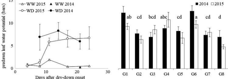
Figure 2a presents the average (across genotypes) of pre-dawn leaf water potential (PLWP) measured once to twice a week along the water shortage period. Water deficit stabilized between six and eight bars 3 days earlier in 2014 compared with 2015 due to the slightly highest cumulative water supply in 2018. Table 3 presents the ANOVA performed on PLWP to evaluate genotype (G), year (Y), date (D) effects, and inter-actions, considering only the last three dates of measurement of each year, that is, the time window within which water

deficit stabilized. G effect was highly significant (p < 0.001). PLWP was then averaged per genotype across these three dates of measurement (as no interaction with the G effect was detected) in order to compare the water deficit underwent by each genotype during this period (Figure 2b). The water defi-cit of G1 and G6 (highest PLWP groups: a and ab classes according to HSD test) significantly differed from that of G2, G7, and G8 (lowest PLWP group: cd and d classes).

3.2 _|

Genotypic variability of stem growth

component traits

3.2.1 _|

Stem level

Genotypic variability was first considered on well‐watered plants at final harvest both at stem and internode levels. Figure 3 presents the genotypic variability exhibited by the eight studied genotypes for key stem growth, development, and biochemical variables, at final harvest in the control treatment only. Table 4 provides the corresponding ANOVA results (Supporting Information Table S2b provides the cor-responding matrix of correlations for biochemical traits only). A significant (p < 0.001) genotype effect was observed on all traits but leaf dry weight (p < 0.01) and stem biomass density

FIGURE 2 (a) Average predawn leaf water potential in the water deficit (WD, average for the eight studied genotypes) and well watered (WW, G1 only) treatments in 2014 and 2015 along the water shortage period (average based on 6–9 plants, i.e., 2–3 plants per block on 3 blocks); (b) average of predawn leaf water potential (bars) for the water deficit period (average on the last three dates of measurement) for the eight studied genotypes on 2 years (2014, 2015) in the WD treatment… The letters provided at the top of the bars correspond to the HSD‐Tukey groups of genotypes over the 2 years. Standard error bars are presented in (a) and (b)

Trait

Mean ANOVA

2014 2015 Y G D G × Y G × D Y × D

Predawn leaf water

potential (bars) 7.0 6.3 ns *** * ns ns *

TABLE 3 Mean values and ANOVA results for predawn leaf water potential measured at the last 3 dates of measurement during the water deficit periods in 2014 and 2015 experiments (Y: year, G: genotype, and D: date effects). p‐values: ‘***’ <0.001; ‘**’ <0.01; ‘*’ <0.05; ‘ns’ nonsignificant

(9)

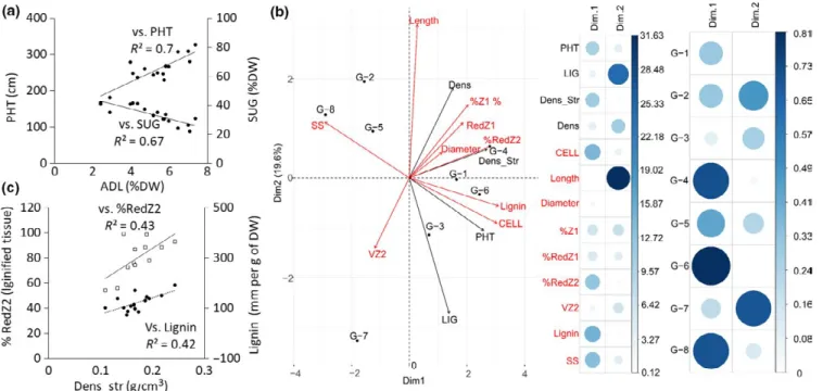
(p < 0.05). Genotypes firstly differed in main stem DW pro-duction (SDW from 28 g for G8 to 181 g for G1), which was largely related to the corresponding variability in PHT (corre-lation coefficient r of 0.8 with SDW; p < 0.001) and LIG (r of 0.74 with SDW; p < 0.01; Figure 3). The genotypes also var-ied significantly for all stem biochemical traits (Table 4 and, for ADL and SUG, Figure 3). ADL (and also NDF, CELL, and HEMI; see Supporting Information Table S2a) was nega-tively correlated with SUG (p < 0.001) and posinega-tively corre-lated with PHT (p < 0.01) across genotypes (Figure 4a).

ADL and CELL genotypic variability was related both to the variation in NDF and to their relative content per NDF unit (Supporting Information Table S2a). By contrast, HEMI variation was only explained by NDF variation (Supporting Information Table S2a). Total and structural stem biomass density exhibited also significant genotype effect (Table 4) and varied, respectively, from 0.16 (G7) to 0.31 g/cm3_(G4)

and 0.13 (G7) to 0.22 g/cm3_{(G4) (Figure 3f). Only TTFLO}

exhibited a year effect (p < 0.001, ca. 150°Cd longer in 2015), LDW (p < 0.01), PHT, tiller DW, and HEMI (p < 0.05). G × Y effects were observed for CELL and NDF (p < 0.001), LDW, SUG, LIG, ADL, TTFLO (p < 0.01), and PHT (p < 0.05).

3.2.2 _|

Internode level

The second internode below the top phytomer was sam-pled for morphological, biochemical, and histochemical

characterizations. At final harvest, significant genotypic vari-ability was also observed at this biological scale except for %Z1 which is the area proportion of the outer zone of the in-ternode (Table 5, cf. Supporting Information Figure S3a for a visual appraisal of the genotypic variation observed for his-tological variables). Strong correlations were highlighted be-tween biochemical variables at internode and stem levels. At internode level, ADL and SUG were, respectively, strongly correlated with Lignin and SS (p < 0.001); these correla-tions being lower, as expected, when the NIRS prediccorrela-tions were obtained from analyses at the stem level (Supporting Information Table S2b).

3.2.3 _|

Multiscale analysis of genotypic

variability

Figure 4b presents a PCA using morphological and bio-chemical traits at the different biological scales studied, at final harvest in the well‐watered treatment only. The number of variables in Figure 4b was reduced with respect to (a) the redundancy of biochemical variables measured at stem and internode levels (Supporting Information Table S2) and (b) their genotypic variability (Tables 4 and 5). The first princi-pal component of the analysis (Dim 1) explained 41.3% of the variability observed among the eight studied genotypes. It was negatively explained by soluble sugar content (SS; correlation coefficient r = −0.87) and positively by PHT and

FIGURE 3 Average (of 3 blocks and 4 plants per block and genotype) of main stem dry weight (SDW) (a), ligulated leaf number (LIG) (b), height (PHT) (c), lignin content estimated through ADL (%DW) and ADL/NDF (% total structural carbohydrate content) (d), sugar content (SUG, %DW) (e), density (g/cm3_{) of total and structural (without soluble sugar content) stem biomass (f), measured at final harvest for the eight studied}

genotypes on 2 years (2014, 2015) in well‐watered conditions. For the different traits, standard error bars corresponding to the variability observed between years and repetitions are indicated

(10)

lignin content (r = 0.74 and 0.9 with Dim 1). These variables were also significantly correlated (Figure 4a, Supporting Information Table S2a). Whereas CELL was also strongly associated with Dim 1 (r = 0.9), histological variables were in general less correlated with this dimension to the excep-tion of %RedZ2 (r = 0.82). %RedZ1 was moderately and similarly correlated with the first (Dim 1) and second (Dim 2) principal components (0.45 and 0.33, respectively). The structural, more than the total, stem density was strongly correlated with Dim 1 (r = 0.76 and 0.46, respectively). Structural stem density was indeed strongly and positively

associated with variables related to internode structural car-bohydrate and lignin contents, (r = 0.65) particularly in Z2 (r = 0.65) (Figure 4c). Dim 2 less explained the genotypic variability studied (19.6%). It was mainly correlated with internode length (r = 0.88) and LIG (r = −0.8 with Dim 2 vs. r = 0.41 with Dim 1). VZ2 and internode diameter were weakly (negatively) associated with Dim 1 and Dim 2. Whereas G4 and G6 were positively (Cos² of 0.72 and 0.82, respectively) and G5 and G8 negatively (Cos² of 0.54 and 0.67) explained by Dim 1, G7 was negatively (Cos² of 0.73) and G2 positively (Cos² of 0.47) correlated with Dim 2.

TABLE 4 Mean values and variance components obtained through ANOVA for morphological and biochemical variables measured at plant level at the end of the water deficit period and at final harvest, on eight genotypes (G), 2 years (Y: 2014, 2015), and 2 water treatments (T: well watered, WW and one‐month water deficit during stem elongation, WD). Average values presented are based on 12 plants (3 blocks, 4 plants per block). SDW, LDW: stem and leaf dry weight; PHT: plant height; LIG: last ligulated leaf rank; ADL: acid detergent lignin; Cell: cellulose content; Hemi: hemicellulose content; Sug: soluble sugars; and NDF: neutral detergent fiber (cell wall content); TTFLO: cumulative thermal time from sowing to flowering; density and structural density refer to stem biomass. p‐values: ‘***’ <0.001; ‘**’ <0.01; ‘*’ <0.05; ‘ns’ nonsignificant >0.05

Trait Date Mean ANOVA 2014 2015 Y G T G × Y G × T Y × T WW WD WW WD TTFLO (sum of °Cd) 956.7 1046.7 1103.8 1227.5 *** *** *** ** ** ns PHT (cm) End stress 138.6 71.9 153.5 82.1 * *** *** ns * ns Harvest 267.2 194.5 255.0 191.3 * *** *** * ns ns

LIG End stress 15.3 12.4 14.9 12.7 ns *** *** ** ns ns

Harvest 20.1 19.3 20.1 18.8 ns *** * ** *** ns Dry weight (g) SDW End stress 36.5 23.1 54.0 30.8 *** *** *** ns ns ** Harvest 103.9 88.2 118.5 82.5 ns *** ** ns ns ns LDW End stress 34.7 25.5 33.0 22.3 ** *** *** ns ** ns Harvest 38.8 40.2 52.1 43.1 ** ** ns ** ns *

Tiller End stress 32.4 16.5 36.2 26.7 ns * * *** ns ns

Harvest 56.0 43.1 100.8 58.1 * *** * ns ns ns Density (g/cm3₎ _Harvest _0.24 _0.25 _0.26 _0.25 _ns _* _ns _ns _ns _ns Structural density (g/cm3₎ Harvest 0.16 0.16 0.17 0.17 ns * ns ns * ns NDF (%DW) End stress 71.5 52.9 66.3 54.3 *** *** *** ns ns *** Harvest 59.0 56.7 55.6 56.8 ns *** ns *** * ***

ADL (%DW) End stress 5.3 2.4 5.0 3.0 ns *** *** * ns **

Harvest 5.5 4.5 5.0 5.0 ns *** ** ** ns **

SUG (%DW) End stress 11.9 22.6 16.7 25.5 *** *** *** ** ns ns

Harvest 32.0 32.1 34.6 32.8 ns *** ns ** ** ns

CELL (%DW) End stress 41.4 28.9 36.3 27.2 *** *** *** ns ns **

Harvest 31.7 29.1 29.5 29.3 ns *** * *** * *

HEMI (%DW) End stress 24.8 21.5 25.0 24.2 *** *** *** *** *** ***

(11)

3.3 _|

Water deficit impact of stem growth

component traits

3.3.1 _|

Stem level

Water deficit (T) significantly reduced SDW at the end of the stress period by 43% and 37%, respectively, in 2014 and 2015 (p < 0.001; Table 4 and Figure 5a). It also reduced LDW, PHT, LIG (p < 0.001; Figure 5b), and tiller DW (p < 0.05). Only PHT and LDW exhibited significant G × T (Figure 5a,b). Water deficit effect was particularly strong on NDF, ADL, HEMI, and CELL (p < 0.001) which were reduced by water deficit (in average by 22, 47, 22, and 8% respectively), by contrast with SUG that was significantly increased (70%; p < 0.001; Figure 5c–f). Among them, only HEMI exhibited G × T (p < 0.001; Table 4 and Figure 5d,e); ADL showed the highest reduction, not only due to the re-duction of NDF but also to its rere-duction per unit of NDF (Figure 5d, Supporting Information Table S2a). CELL duction was largely explained by NDF reduction (same re-duction of 22%, see correlations in Supporting Information Table S2a). HEMI reduction was lower than that of NDF as it increased in % of NDF (HEMI/NDF, Figure 5f). ADL/NDF,

CELL/NDF, and HEMI/NDF showed G × T (p < 0.01, not shown).

Figure 6a shows a PCA of the response rates to water defi-cit (Eq3) of morphological and biochemical traits considered at the end of the water deficit period in 2014 and 2015. Traits for this PCA were selected based on their genotypic variations and/or correlations (Supporting Information Table S2a). Dim 1 (explaining 35.5% of the variation observed) was strongly and positively explained by the response rate to water deficit of NDF, ADL, LIG, and PHT (r of 0.82, 0.84, 0.63, and 0.63, respectively) and negatively by the response rate of SUG (r of −0.58). The correlations between the reductions of PHT and ADL or NDF were, however, low and nonsignificant (r < 0.2, p > 0.4) by contrast with those between SUG and ADL or NDF (r = −0.56 (p < 0.05) with ADL; r = −0.65 (p < 0.01) with NDF). Dim 2 explained 25.2% of the observed variation and was positively explained by PHT, IN‐2 length (r = 0.71 for both) and negatively by HEMI/NDF (r = −0.62). SDW was equally and moderately explained by Dim 1 and Dim 2 (r of 0.4 and 0.45, respectively). Only G7 had high and positive coordinates on Dim 1 (Cos² of 0.61). G3 and G4 had high coordinates on Dim 2 (Cos² of 0.77 and 0.71, respectively). PLWP was not correlated with Dim 1 and Dim 2.

FIGURE 4 (a) Relation between stem lignin content (ADL) and height (PHT) or sugar content (NIRS prediction: SUG). (b) PCA for stem morphological variables (PHT, leaf number LIG, density of total and structural stem biomass: respectively Dens and Dens_Str, in g/cm3₎

and internode variables: morphological (length, diameter), histological (percentage of red tissue in inner zone Z2 (%RedZ2) and outer zone Z1 (%RedZ1), percentage of Z1 area (%Z1), density of vascular bundles in Z2 (VZ2, mm−2_{), biochemical (Lignin and soluble sugar SS contents}

in mg/g of DW), and NIRS prediction of cellulose content (CELL %DW). Internode variables refer to the second internode below the flag leaf phytomer on the main stem and are indicated in italics in (b). The two‐first dimensions (Dim 1 and Dim 2) of the PCA are considered. The centroid for each genotype is positioned (black circles). Below the PCA are presented the contributions (%) of each variable and the Cos² of each genotype on Dim 1 and Dim 2. The size and darkness of circles for each factor refer to the scale on the right. (c) Relation between stem Dens_str and %RedZ2 or Lignin content in IN‐2. Data from the well‐watered treatment at final harvest in 2014 and 2015 for the eight studied genotypes. Each point in (a) and (c) is the average of three blocks per genotype and year

(12)

TABLE 5 Mean values and variance components obtained through ANOVA for morphological, histological, and biochemical variables measured at 2 stages (end of the water deficit period (end stress) and final harvest), for different internode levels on the main stem of the eight studied genotypes (G), on 2 years (Y: 2014, 2015) under 2 water treatments (T:well watered, WW; 1‐month water deficit during stem elongation, WD) in the field. ADL: acid detergent lignin content (NIRS predicted); CELL: cellulose content (NIRS predicted); SUG: soluble sugar content (NIRS predicted); SS and Lignin: soluble sugar and lignin contents; PerZ1: outer zone area (Z1) in % of internode section area; PerSclZ1: percentage of sclerenchyma tissue (red stained) in Z1 area; VZ2: density of vascular bundles in central zone (Z2); PerRedZ2 percentage of red stained (lignified) tissue in Z2 area. Each value in the table is the average of 6–12 internodes (3 blocks with 2–4 plants per block depending on the trait). Values are provided for the second (IN‐2) and sixth (IN‐6, harvest) internodes below the last ligulated leaf phytomer. IN+2 is the second internode expanded above the phytomer of the last ligulated leaf at the end of the stress period on stressed plants. (s) indicates that a given variable was compared for the same rank (counted from the bottom of the stem and taking as reference the rank on the stressed plants) on stressed and control plants (p‐values: ‘***’ <0.001; ‘**’ <0.01; ‘*’ < 0.05; ‘ns’ (nonsignificant) >0.05)

Trait Stage Rank IN

Mean ANOVA

2014 2015

Y G T G × Y G × T Y × T

WW WD WW WD

Length (cm) End stress IN‐2 (s) 19.29 13.62 21.15 14.85 ns *** *** ns ns ns

IN+2 (s) 23.24 19.18 20.37 17.02 ns *** ns ns ns ns

Harvest IN‐2 18.03 15.63 15.15 14.40 ns *** ns ns * ns

IN‐6 22.66 17.06 18.86 16.21 ns *** ns * ns ns

Diameter (mm) End stress IN‐2 (s) 16.03 15.86 18.03 17.54 * *** ns ns ns ns

Harvest IN‐2 13.26 12.96 13.02 12.31 ns *** ns ** ns ns

IN‐6 14.28 13.83 14.29 14.26 ns *** ns ns ns ns

NDF (%DW) End stress IN‐2 ‐ ‐ 56.30 44.24 ‐ *** *** ‐ ns ‐

Harvest IN‐2 54.73 51.48 49.04 48.74 ** *** ns *** * ns

IN‐6 57.11 49.21 48.58 47.60 *** *** *** *** *** **

ADL (%DW) End stress IN‐2 ‐ ‐ 2.90 1.86 ‐ *** ** ‐ ns ‐

Harvest IN‐2 3.97 3.20 3.32 3.14 ns *** ns *** ns ns

IN‐6 5.27 4.08 4.20 3.82 ns *** ** *** *** *

CELL (%DW) End stress IN‐2 ‐ ‐ 30.22 22.92 ‐ *** *** ‐ ns ‐

Harvest IN‐2 27.68 25.46 24.85 24.52 ns *** ns *** ns ns

IN‐6 30.67 25.44 26.15 25.32 ** *** ** *** *** **

HEMI (%DW) End stress IN‐2 ‐ ‐ 23.20 19.46 ‐ *** *** ‐ *** ‐

Harvest IN‐2 23.13 22.83 21.26 20.48 *** *** ns *** * ns

IN‐6 21.17 19.69 18.61 18.00 *** *** ** ** *** ns

SUG (%DW) End stress IN‐2 ‐ ‐ 25.32 32.19 ‐ *** ** ‐ ** ‐

Harvest IN‐2 32.47 33.44 38.85 38.62 *** *** ns *** * ns

IN‐6 30.20 35.68 39.00 39.71 * *** ns *** *** ***

Lignin (mg/g

DW) End stress_Harvest IN‐2_IN‐2 _123.76‐ _114.27‐ 121.97_109.03 _121.35103.09 _ns‐ _**** _ns** _*‐ _nsns ‐_*

IN‐6 134.72 117.63 119.23 115.51 ns *** ns ** * *

SS (mg/g DW) End stress IN‐2 ‐ ‐ 245.66 274.54 ‐ *** ns ‐ ns ‐

Harvest IN‐2 278.73 314.64 316.25 291.91 * *** ns *** ns *

IN‐6 293.04 365.29 314.41 316.01 ns *** * *** ** ***

%Z1 (%area) End stress IN‐2 ‐ ‐ 17.03 20.95 ‐ ns *** ‐ ** ‐

Harvest IN‐2 17.86 17.56 16.35 16.40 ** ns ns * ns ns

%RedZ1 (%Z1

area) End stress_Harvest IN‐2_IN‐2 _43.76‐ _40.68‐ 14.75_23.39 _21.2610.60 _***‐ _***** _ns* _ns‐ _nsns ‐_ns

VZ2 (nb/mm2₎ _{End stress} _IN‐2 _‐ _‐ _1.30 _1.13 _‐ _*** _* _‐ _** _‐

Harvest IN‐2 1.61 1.64 1.42 1.61 ns *** ns ns ns ns

%RedZ2 (%Z2

(13)

3.3.2 _|

Internode level

Table 5 presents the average values and variance components for variables estimated on IN‐2 (length and diameter in both years; other traits only in 2015). IN‐2 length was signifi-cantly reduced by drought (p < 0.001; 28%), whereas diam-eter was not (Figure 7 for G1 and G8). Similarly to the stem level, a significant decrease by water deficit of NDF (−21%; p < 0.001), CELL (−24%; p < 0.001), HEMI (−16%; p < 0.001), and ADL (−34%; p < 0.01) was observed. Lignin content was also reduced but less than ADL (−15%, p < 0.01), whereas SUG and SS were equally increased (+27 vs. +28%, significant only for SUG [p < 0.01]). Histological traits significantly responded to water deficit: %RedZ1 and %RedZ2 decreased (−26% (p < 0.05) and −61% (p < 0.001), respectively). %Z1 and VB2 increased, respectively, by 23% (p < 0.001) and 13% (p < 0.05) (see Supporting Information Figure S3b for image examples). G × T were significant on HEMI (p < 0.001), SUG, VB2, %Z1 (p < 0.01), and %RedZ2 (p < 0.05).

To summarize, water deficit reduced plant height (PHT) and stem dry weight (SDW) through the reduction of the number of phytomers developed on the main stem (LIG), of the internode length but not of the diameter (IN‐2). This was associated at plant stem and internode levels with an in-crease in soluble sugars and a dein-crease in fiber contents, lig-nin in particular, as represented by NDF, ADL/DNF, Liglig-nin, %RedZ1, and %RedZ2. The genotypes that better‐maintained growth (PHT, SDW) did not systematically better maintain fiber content (e.g., G4).

3.4 _|

Response to rewatering

3.4.1 _|

Stem level

At final harvest, water deficit effect was still significant on tiller DW (p < 0.05), SDW (p < 0.01), height (PHT, p < 0.001), and LIG (p < 0.05) (Table 4). Only LIG exhib-ited G × T (p < 0.001), which was related to the fact that the genotypes that did not (or partially) flower (G7 for both years and, in 2015, G1 and G6) did not yet recover phytomer num-ber in the stressed treatment compared with the control treat-ment (cf. Supporting Information Figure S5). Stem structural biomass density, SUG, and NDF did not show any treatment effect, in contrast to ADL (p < 0.01), CELL (p < 0.05), and HEMI (p < 0.001). G × T effects were observed for stem structural density, NDF (p < 0.05), SUG, and HEMI (p < 0.05; Table 4).

The recovery rate of traits measured at plant level was computed (Eq4). The genotypes showed variability in their recovery capacities for all studied traits, but they were higher for SDW, PHT, and LIG (Supporting Information Figures S4 and S5). The covariation among trait recoveries was evaluated using a PCA (Figure 6b). Dim 1 explained 33% of observed variation. It was negatively explained by the recovery of LIG (r of −0.67), SUG (r of −0.91) and positively by the recovery of NDF (r of 0.93). Only SUG and NDF recoveries were significantly and negatively cor-related (r of −0.954, not shown). Dim 2 explained 26.3% of observed variability and was mainly explained by the recovery rate of ADL (r = 0.8), HEMI/NDF (r = 0.87),

FIGURE 5 Average response to drought (Resp%, Equation 3) and standard deviation (between years) estimated for the eight genotypes at the end of the stress period: (a) Stem dry weight (SDW); (b) LIG (last ligulated leaf rank on the main stem); (c) NDF (neutral detergent fiber: NIRS prediction of total structural carbohydrate content in %DW); (d) ADL (NIRS prediction of lignin content in the stem in %DW or in %NDF [total fiber content]) (e) SUG (NIRS prediction of soluble sugar content in the stem in %DW); (f) HEMI (NIRS prediction of hemicellulose content in the stem in %DW or in %NDF)

(14)

FIGURE 6 Principal component analysis of: (a) the response to water deficit (Equation 3) of morphological and NIRS predicted biochemical variables measured on the main stem at the end of the water deficit period: SDW (stem dry weight, g), PHT (plant height, cm), LIG (ligulated leaf number), ADL (acid detergent lignin content, %DW), HEMI/NDF (hemicellulose content, % of total fiber content NDF), SUG (soluble sugar content, %DW); length refers to the second internode below the phytomer of the top ligulated leaf on the main stem of stressed plants). (b) The recovery rate under rewatering (Equation 4) of these variables. Length refers to the second internode expanded after rewatering onset. PLWP (predawn leaf water potential) and TTFLO (thermal time cumulated from sowing to flowering, only in B) are supplementary variables (blue). Variables at internode level are indicated in red. The centroid of each genotype (G1–G8) is positioned (black points). Below each PCA are presented the corresponding contributions (%) for each variable and the Cos² (for each genotype) to Dim 1 and Dim 2; the size and darkness of circles for each factor refer to the scale on the right

(15)

and PHT (r = 0.61). Only G4 and G7 exhibited high coor-dinates (with Dim 1: positive for G4 with a Cos² of 0.74; negative for G7 with Cos² of 0.82). SDW recovery moder-ately correlated with the two‐first dimensions. It was also the case of TTFLO and PLWP used here as supplementary variables. No significant correlations were found between the genotypic response to water deficit and the recovery

of studied variables (not shown), to the exception of ADL showing a positive correlation (r of 0.78, p < 0.001).

3.4.2 _|

Internode level

Table 5 presents the variance components of morphological and histochemical variables measured at organ level at final

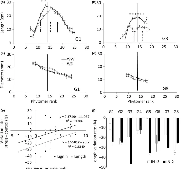
FIGURE 7 Internode morphological and biochemical trait variation with the water availability treatments (WW: well watered, WD: water deficit) measured at final harvest: Profile of (a, b) length and (c, d) diameter averaged over the 2 years. Each point is the average of 18 plants with corresponding standard deviations. Bold vertical arrow corresponds to the position of the 6th internode below the flag leaf phytomer (IN‐6) also sampled for biochemical analyses at final harvest. Dotted and dashed vertical arrows represent, respectively, internodes of relative rank +2 (IN+2) and −2 (IN‐2) estimated from the rank of the youngest expanded leaf phytomer at rewatering onset, (considered at 0 and represented by the vertical black bar). Stars indicate the internode ranks at which the water deficit effect is significant (p < 0.05). (e) Relationship between IN‐6 relative rank and its variation rate (Resp%) in stressed vs. control plants of Lignin content and length. Each point is an average value for a given genotype any year. (f) IN+2 and IN‐2 Resp% for length for each studied genotype, in average over the 2 years. Standard deviations are presented

(16)

harvest, on IN‐2 and IN‐6. Only IN‐6 exhibited T and G × T (and Y × T) effects on most of studied biochemical traits. Indeed, by contrast with IN‐2 that expanded under rewater-ing for all genotypes, IN‐6 had a different fate dependrewater-ing on genotype phenology: the shorter the cycle duration, the lower the number of internodes remaining to expand after the water deficit period and before flowering. In this case, IN‐6 could be an internode having expanded under stress. This is schematized in Figure 1 and illustrated in Figure 7a,b for two genotypes contrasting for cycle duration and internode number.

To evaluate to which extent the genotypic variation in IN‐6 response to the water treatment was explained by plant phenology, this variation was expressed as a function of IN‐6 age at the end of the stress period. This age was com-puted relatively to the rank of the top internode at the end of the stress period (referred as 0 and identified by the vertical plain line in Figure 7a,b). This is presented in Figure 7e for IN‐6 length and ADL. Both were positively related to the age of IN‐6 at the end of the stress period (r of 0.4), but not significantly (p < 0.1). This suggests that when IN‐6 fully developed during the water deficit period (negative relative age), it did not recover up to final harvest; conversely when it developed after rewatering, the highest its relative rank the lowest the water deficit effect. Nevertheless, the nonsig-nificance of this correlation suggests that plant phenology poorly explained the variation observed on IN‐6 response to water.

The genotypes also varied in the number of internodes to be expanded under rewatering before internode size in stressed plants became comparable to the control plants. For example, in G1, the second internode developed after rewa-tering (IN+2, Figure 7a,b) already recovered a length similar to control plants. By contrast, in G8, the internodes devel-oped under rewatering never recovered in stressed plants the length observed in control plants. IN+2 was chosen accord-ingly to compare genotypes regarding this recovery capac-ity. Its response to water treatment in terms of final length is plotted in Figure 7f, showing a strong genotypic variability (from −35% for G8 to −1% for G5). This genotypic vari-ability was largely confirmed at whole stem level (PHT in Supporting Information Figure S5) where, for example, G1 and G4 exhibited among the best recovery capacities and G6 or G8 among the worst. This was not that clear when looking at SDW that showed a different ranking of genotype recov-eries (Supporting Information Figure S5): As suggested by Figure 6b, the recovery of SDW is more complex and should depend on both growth and biochemical recovery traits.

In Figure 7f, IN+2 length response to water deficit was plotted aside that of IN‐2 (Figure 7a,b), revealing the absence of correlation between these two variables (r = 0.3, linear re-gression not shown), similarly to that observed at whole stem level.

4 _|

DISCUSSION

4.1 _|

Genotypic covariations exist among

stem biomass component traits

The present study aimed to evaluate to which extent traits contributing to stem biomass growth and biochemical com-position at different biological scales (co‐)vary with the genotype and water conditions in sorghum. The eight stud-ied genotypes contrasted for stem biomass accumulation and component traits related to stem growth. Covariations were pointed out between these types of traits. In particular, plant height was positively correlated with stem structural carbo-hydrate and lignin contents and negatively correlated with stem soluble sugar content. Accordingly, the tallest geno-types were the most lignified and the less sweet. This positive correlation between stem height and fiber content was previ-ously reported but with an extent largely dependent on the ge-netic material studied (Carvalho & Rooney, 2017; Maria G. Salas Fernandez, Becraft, Yin, & Lübberstedt, 2009). Shukla, Felderhoff, Saballos, and Vermerris (2017) compared tall, sweet sorghum genotypes to their converted (dwarf) versions and could suggest that stalk sweetness was partially inde-pendent of stem height. As stem soluble sugar and cell wall contents appeared inversely proportional in the present study as well as in the study reported by McKinley et al. (2018; in an energy‐sorghum diversity panel), it would mean that stem height and lignin content are also partially independent which gives larger breeding opportunities. Interestingly, the variation in stem biomass structural density could be related to stem lignin content and more particularly in the inner zone of the internode. This gives evidence that histological studies provide a better understanding of the component traits affect-ing biomass quality (Legland et al., 2017) and should help to better monitor this complex trait in the course of breeding programs.

4.2 _|

Water status effect on stem biomass

accumulation is genotype and trait dependent

4.2.1 _|

Response to water deficit

The eight studied genotypes exhibited a reduction of the length, the number, and the cell wall content and an increase in soluble sugar accumulation of internodes expanded dur-ing the water deficit period. This resulted in reduced stem height and dry weight. As recently reported by Perrier et al. (2017) on two genealogically related sorghum hybrids, water deficit did not affect internode diameter but length. This is in line with the effect of water deficit effect on expanding leaves in cereals such as maize in which cell elongation is more impacted than cell division (Lacube et al., 2017). Leaf length and width were also measured in the present study and

(17)

confirmed this result (not shown). It will be interesting to ex-plore whether the genetic determinisms of leaf and internode length sensitivity to water deficit are linked in larger diversity panels.

The more a genotype reduced stem cell wall content the more it accumulated soluble sugars. The role of soluble sugar accumulation contributing, in water deficit conditions, to cell osmoregulation and tissue turgor maintenance was already reported (de Souza, Cocuron, Garcia, Alonso, & Buckeridge, 2015). The role of nonstructural carbohydrate remobilization from the stem to the grains in cereals at grain filling stage under water deficit conditions was also demonstrated (e.g., in wheat [Yáñez, Tapia, Guerra, & del Pozo, 2017; ]). Tovignan, Fonceka et al. (2016) reported that the maintenance of soluble sugar content in the stem of sweet sorghum under postflowering drought was conditioned by stay‐green ability and thus the capacity of a given genotype to carry on assim-ilating C. An increase in stem sugar content can be also the result of a reduction of reproductive C sinks in the plant and thus of stem sugar remobilization. This was reported, for ex-ample, by (Gutjahr et al., 2013) comparing sweet sorghum genotypes in their fertile and sterile (no grain filling) ver-sions. In the present study, the increase in soluble sugar accu-mulation in stem internodes was proportional to the reduction in cell wall content that also represents a strong C sink for the plant (Cabane et al., 2012). Accordingly, this increase in soluble sugar content could be considered as the result of a positive C source‐sink balance in the stem.

No clear correlation was found in the present study be-tween the reduction by water deficit of stem cell wall content and length, although both should be related to the slowing of internode elongation. Indeed, Perrier et al. (2017) demon-strated that cell wall and more particularly lignin and cellu-lose deposition are progressive along internode elongation, whereas in the same time, hemicellulose content is more constant. In the present study, lignin and cellulose contents were negatively impacted, whereas hemicellulose in %NDF increased in the stem internodes of stressed plants compared with the control plants analyzed at the end of the stress pe-riod. This is in line with the pattern exhibited by younger, expanding internodes compared to older, expanded ones as reported by Perrier et al. (2017). Preliminary results at in-ternode tissue level suggested that the reduction of inin-ternode lignin content by water deficit occurred both in the inner part (parenchyma Z2) and in the outer (sclerenchyma Z1) part of the internode, but more strongly in Z2 (Table 5: reduction in average of 60% and 40%, respectively, for %RedZ2 and %RedZ1). This result corroborates that reported by Perrier et al. (2017) only for %RedZ1 and two hybrids. %Z1 (area proportion of the outer zone in the internode section) was by contrast increased by water deficit, reinforcing the idea that, in general, water deficit affects more the lignification in the parenchyma than in the sclerenchyma. This corroborates

results recently reported in maize (El Hage et al., 2018). In addition, as the sclerenchyma plays a key role in stem lodging resistance in tall herbaceous plants, it makes sense that, in an environmental situation reducing cell wall lignification, this particular tissue should be relatively less affected (Zheng et al., 2017).

The reduction by water deficit of cell wall content to the benefit of soluble sugars was already shown on grass crops as miscanthus (van der Weijde et al., 2017). The same authors also reported that the drought tolerance for biomass composi-tion and produccomposi-tion was independent in this species and sug-gested it is an advantage for breeding. In the present study, genotypic variation was pointed out both for stem biomass production and for composition responses to water deficit. Stem dry weight reduction by water deficit was explained at the end of the stress period by the reduction in both internode length (but not diameter) and number (Figure 6a). The biomass production reduction induced by the water deficit was weakly correlated with the variation in stem composition. Preliminary results at internode level suggested, however, a partial linkage between growth and composition responses to water deficit (Figure 7e). Stem density could be computed only at final har-vest (when internode size profiles were measured on the main stem), that is, when water deficit effect was not significant. It was thus not possible to check whether the relationship be-tween stem structural density and lignin content (particularly in Z2) was maintained at earlier stages under water deficit. It will be interesting to further explore these covariations within a larger genetic diversity and considering histochemical traits separately for the Z1 and Z2 internode regions. Such results will have implications on the breeding strategies to be adopted for biomass sorghum in drought‐prone environments.

4.2.2 _|

Response to rewatering

This study showed that biomass sorghum genotypes dif-fered in their capacity to recover growth and cell wall deposition after a water deficit period (Figures 6b and 7e,f and Supporting Information Figures S4 and S5). The genotypes that better recovered for stem biomass growth (PHT, SDW) did not necessarily better recover for cell wall residue contents (Figure 6b; Supporting Information Figure S5). The recovery in stem lignocellulosic composi-tion was much less variable among genotypes compared to that of growth‐related traits (Supporting Information Figure S5). Genotype recovery at stem level was in part dependent on cycle duration that conditioned the propor-tion of internodes grown under water deficit vs. rewatering. This was accentuated by the fact that internodes expanded under water deficit did not recover neither for length nor for lignocellulosic content. To our knowledge, these results on stem growth recovery are original and should be ex-tended to larger genetic diversity.