HAL Id: hal-00730188
https://hal.archives-ouvertes.fr/hal-00730188
Submitted on 7 Sep 2012
HAL is a multi-disciplinary open access
archive for the deposit and dissemination of
sci-entific research documents, whether they are
pub-lished or not. The documents may come from
teaching and research institutions in France or
abroad, or from public or private research centers.
L’archive ouverte pluridisciplinaire HAL, est
destinée au dépôt et à la diffusion de documents
scientifiques de niveau recherche, publiés ou non,
émanant des établissements d’enseignement et de
recherche français ou étrangers, des laboratoires
publics ou privés.
Quaternionic Sparse Approximation
Quentin Barthélemy, Anthony Larue, Jerome Mars
To cite this version:
Quentin Barthélemy, Anthony Larue, Jerome Mars. Quaternionic Sparse Approximation. AGACSE
2012 - 5th conference on Applied Geometric Algebras in Computer Science and Engineering, Jul 2012,
La Rochelle, France. Paper#4, p1-11. �hal-00730188�
Quaternionic Sparse Approximation
Quentin Barth´elemy, Anthony Larue and J´erˆome I. Mars
Abstract In this paper, we introduce a new processing procedure for quater-nionic signals through consideration of the well-known orthogonal matching pur-suit (OMP), which provides sparse approximation. We present a quaternionic ex-tension, the quaternionic OMP, that can be used to process a right-multiplication linear combination of quaternionic signals. As validation, this quaternionic OMP is applied to simulated data. Deconvolution is carried out and presented here with a new spikegram that is designed for visualization of quaternionic coefficients, and finally this is compared to multivariate OMP.
1 Introduction
In signal processing, some tools have been recently extended to the quaternion space H. For example, we can cite quaternionic correlation for vector images [8], quater-nionic adaptive filtering [11], quaterquater-nionic independent component analysis [13], and blind extraction of quaternionic sources [5].
For the sparsity domain, sparse approximation algorithms [12] are given for real or complex signals. To our knowledge, these have not been applied to quaternionic signals. Considering orthogonal matching pursuit (OMP) [9], we present an exten-sion to quaternions. This algorithm, which is termed quaternionic OMP (Q-OMP), can be used to process quadrivariate signals (and thus including trivariate signals).
Quentin Barth´elemy
CEA-LIST, PC 72, 91191 Gif-sur-Yvette Cedex, France, e-mail: [email protected] Anthony Larue
CEA-LIST, PC 72, 91191 Gif-sur-Yvette Cedex, France, e-mail: [email protected] J´erˆome I. Mars
GISPA-Lab, 11 rue des math´ematiques BP46, 38402 Saint Martin d’H`eres, France, e-mail: [email protected]
For the quaternionic signal y∈ HN of N samples and a dictionaryΦ ∈ HN×Mof
Matoms{φm}Mm=1, the decomposition of the signal y is carried out on the dictionary
Φ such that: y= M
∑
m=1 φmxm+ ε , (1)assuming xm∈ H are the coding coefficients and ε ∈ HN the residual error. It is this
right-multiplication model that will be considered for the following quaternionic sparse approximation. This model is used in different real-world applications, such as wind forecasting and colored images denoising [11], and in blind source extrac-tion of EEG mixtures [5].
In this paper, we first consider sparse approximation and the OMP algorithm in Section 2. We then present the quaternionic extension Q-OMP in Section 3. In Sec-tion 4, we specify our work for the shift-invariant case, and we introduce a new visualization tool for quaternionic sparse decompositions. Finally, in Section 5, the Q-OMP is applied to deconvolute simulation data, and then compared to multivari-ate OMP (M-OMP).
2 Sparse Approximation
The sparse approximation principle and the OMP algorithm are presented in this section, with processing of only complex signals.
2.1 Principle and existing algorithms
Considering a signal y∈ CN of N samples and a dictionaryΦ ∈ CN×Mof M atoms
{φm}Mm=1, the decomposition of the signal y is carried out on the dictionaryΦ such
that:
y= Φx + ε , (2)
assuming x∈ CMare the coding coefficients andε ∈ CN the residual error. The
dic-tionary is normed, which means that its columns (atoms) are normed, so that coef-ficients x reflect the energy of each atom in the signal. Moreover, the dictionary is said to be redundant when M> N.
One way to formalize the decomposition under the sparsity constraint is: minxk y − Φx k22 s.t. kxk0≤ K , (3)
where K≪M is a constant and kxk0theℓ0pseudo-norm that is defined as the
cardi-nality of x. This formulation is composed of a data-fitting term and a term of sparsi-fication, to obtain the sparsest vector x. Pursuit algorithms [12] tackle sequentially (3) increasing K iteratively, although unfortunately this optimization is nonconvex:
that means the obtained solution can get stuck in a local minimum. Nevertheless, these algorithms are fast when searching very few coefficients. Among the multiple ℓ0-Pursuit algorithms, we can cite the well-known matching pursuit (MP) [6], its
orthogonal version, OMP [9] and multivariate OMP (M-OMP) [1] for treating mul-tivariate signals. Note that another way consists of relaxing the sparsification term from anℓ0norm to anℓ1norm, which gives a convex optimization problem [12].
2.2 Review of Orthogonal Matching Pursuit
We present the step-by-step OMP that is introduced in [9] with complex signals. Given a redundant dictionaryΦ, OMP produces a sparse approximation of a signal y(Algorithm 1).
After an initialization (step 1), OMP selects at the current iteration k the atom that produces the absolute strongest decrease in the mean square error (MSE) εk−1
2 2.
This is equivalent to selecting the atom that is the most correlated with the residue. The inner products between the residueεk−1and atomsφ
mare computed (step 4).
The selection (step 6) searches the maximum of their absolute values to determine the optimal atomφmk, denoted dk. An active dictionary Dk∈ CN×kis formed, which
collects all of the selected atoms (step 7). Coding coefficients xkare computed via the orthogonal projection of y on Dk (step 8). This is often carried out recursively by different methods using the current correlation value Ckmk: QR factorization [3],
Cholesky factorization [2], or block matrix inversion [9]. The obtained coefficients vector xk= [xm1; xm2... xmk]T is reduced to its active (i.e. nonzero) coefficients, with
(.)T denoting the transpose operator.
Different stopping criteria (step 11) can be used: a threshold on k for the number of iterations, a threshold on the relative MSE (rMSE) εk
2
2/kyk
2
2, or a threshold on
the decrease in the rMSE. At the end, the OMP provides a K-sparse approximation of y: ˆ yK= K
∑
k=1 xmkφmk. (4)Used thereafter, M-OMP [1] deals with the multivariate signals acquired simul-taneously.
3 Quaternionic Orthogonal Matching Pursuit
In this section, we present the Q-OMP, the quaternionic extension of the OMP. As mentioned above, different implementations of the OMP projection step exist. In the following, we have chosen to extend the block matrix inversion method [9]. We first outline the quaternionic space and notations, and we then detail the Q-OMP algorithm.
Algorithm 1 : x= OMP (y, Φ) 1: initialization : k= 1, ε0= y, dictionary D0= ∅ 2: repeat 3: for m← 1, M do 4: Inner Products : Ckm← εk−1, φm 5: end for
6: Selection : mk← arg max m Cmk 7: Active Dictionary : Dk← Dk−1∪ φ mk
8: Active Coefficients : xk← arg min x y−Dkx 2 2 9: Residue :εk← y − Dkxk 10: k← k + 1 11: until stopping criterion
3.1 Quaternions
The quaternionic space, denoted as H, is an extension of the complex space C using three imaginary parts [4]. A quaternion q∈ H is defined as: q = qa+ qbi+ qcj+
qdk, with qa, qb, qc, qd∈ R and with the imaginary units defined as: i j = k, jk = i,
ki= j and i jk = i2= j2= k2= −1. The quaternionic space is characterized by its
noncommutativity: q1q26= q2q1. The scalar part is S(q) = qa, and the vectorial part
is V(q) = qbi+ qcj+ qdk. If its scalar part is null, a quaternion is said to be pure
and full otherwise. The conjugate q∗is defined as: q∗= S(q) − V (q) and we have (q1q2)∗= q2∗q1∗.
Now considering quaternionic vectors q1, q2∈ HN, we define the inner product
as:hq1, q2i = q2Hq1, with(.)Hdenoting the conjugate transpose operator. The
asso-ciatedℓ2norm is denoted byk.k2. Note that an alternative definition can be chosen:
hq1, q2i = qH1q2, which is only the conjugate of the previous one.1
In the previous section, OMP was explained for complex variables with the tradi-tional left-multiplication between scalars and vectors. Due to the noncommutativity of quaternions, only the right-multiplication given in Eq. (1) will be considered in the following. Moreover, the quadrivariate data studied are filled in the full quater-nionic variables thereafter.
3.2 Algorithm description
Owing to noncommutativity, the variables order is now crucial. The description of the Q-OMP algorithm is similar to Algorithm 1 (we have taken care to already give the appropriate parameter order in the OMP algorithm), assuming quaternionic signals and the use of right-multiplication. In this section, the changes are detailed, and in particular, the orthogonal projection.
1Note also that the inner product in RN×4:hq
1, q2i=S(qH1q2), which is often used for quaternionic
The inner product εk−1, φm (step 4) remains the expression to maximize to
select the optimal atom (see Appendix). It is now the quaternionic inner product de-fined in Section 3.1. Coefficients xk(step 8) are calculated by orthogonal projection:
the recursive procedure [9] is extended to quaternions and with right-multiplication, as is described below (for normed kernels). Foremost, Ak is defined as the Gram
matrix of the active dictionary Dk−1:
Ak= (Dk−1)HDk−1= hd1, d1i hd2, d1i . . . hdk−1, d1i hd1, d2i hd2, d2i . . . hdk−1, d2i .. . ... . .. ... hd1, dk−1i hd2, dk−1i . . . hdk−1, dk−1i . (5)
At iteration k, the recursive procedure for the orthogonal projection is computed in seven stages:
1: vk= (Dk−1)Hdk= [ hdk, d1i ; hdk, d2i ... hdk, dk−1i ]T ,
2: bk= A−1k vk,
3:β = 1/(kdkk2− vHkbk) = 1/(1 − vHkbk) ,
4:αk= Cmkk· β .
To provide the orthogonal projection, coefficients xmi of vector xk are corrected at
each iteration. Adding a superscript (to coefficients xmi) denotes the iteration, and
the update is:
5: xkmi= xk−1mi − bkαk, for i= 1 .. k−1 ,
6: xkmk= αk.
The Gram matrix update is given by:
Ak+1= " Ak vk vHk 1 # (6)
and using the block matrix inversion formula, we obtain its left-inverse:
7 : A−1k+1= " A−1k + β bkbHk −β bk −β bH k β # . (7)
For the first iteration, the procedure is reduced to: x1
m1= Cm11 and A1= 1.
As Algorithm 1, and with the described modifications, the Q-OMP provides a K-sparse approximation of y: ˆ yK= K
∑
k=1 φmkxmk. (8)4 The shift-invariant case and the spikegram
In this section, we focus on the shift-invariant case, and a new spikegram for quater-nionic decompositions is introduced.
4.1 The shift-invariant case
In the shift-invariant case, we want to sparsely code the signal y as a sum of a few short structures, named kernels, that are characterized independently of their positions. This is usually applied to time series data, and this model avoids the block effects in the analysis of largely periodic signals, and provides a compact kernel dictionary [10].
The L shiftable kernels of the compact dictionaryΨ are replicated at all of the positions, to provide the M atoms of the dictionaryΦ. The N samples of the signal y, the residueε, and the atoms φm are indexed2 by t. The kernels {ψl}Ll=1 can
have different lengths. The kernelψl(t) is shifted in τ samples to generate the atom
ψl(t − τ): zero-padding is carried out to have N samples. The subset σlcollects the
active translationsτ of the kernel ψl(t). For the few kernels that generate all of the
atoms, Eq. (2) becomes:
y(t) = M
∑
m=1 φm(t) xm+ ε(t) = L∑
l=1∑
τ∈σl ψl(t−τ) xl,τ+ ε(t) . (9)To sum up, in the shift-invariant case, the signal y is approximated as a weighted sum of a few shiftable kernelsψl.
The Q-OMP algorithm is now specified for the shift-invariant case. The inner product between the residueεk−1 and each atomφ
m (step 4) is now replaced by
the correlation with each kernelψl. Quaternionic correlation is defined in [8],
al-though with the alternative inner product. In our case, the non-circular quaternionic correlation between quaternionic signals q1(t) and q2(t) is:
Γ{q1, q2} (τ) = hq1(t), q2(t − τ)i = qH2(t − τ) q1(t) . (10)
The selection (step 6) determines the optimal atom that is now characterized by its kernel index lkand its positionτk. The orthogonal projection (step 8) gives the
vector xk=hxl1,τ1; xl2,τ2... xlk,τk
iT
. Finally, Eq. (8) of the K-sparse approximation becomes: ˆ yK= K
∑
k=1 ψlk(t−τk) xlk,τk. (11)2Note that a(t) and a(t − t
0) do not represent samples, but the signal a and its translation of t0
4.2 The spikegram for quaternionic decompositions
We now explain how to visualize the coefficients obtained from a shift-invariant quaternionic decomposition. Usually, real coding coefficients xl,τ are displayed by
a time-kernel representation called a spikegram [10]. This condenses three indica-tions:
• the temporal position τ (abscissa), • the kernel index l (ordinate),
• the coefficient amplitude xl,τ (gray level of the spike).
This presentation allows an intuitive readability of the decomposition. With complex coefficients, the coefficient modulus is used for the amplitude, and its argument gives the angle, which is written next to the spike [1]. This coefficient presentation provides clear visualization.
To display quaternionic coefficients and to maintain good visualization, each quaternionic coefficient is written such that:
xl,τ= xl,τ · ql,τ and ql,τ= eiθ
1
l,τ· ekθl,τ2 · ejθl,τ3 , (12)
with the coefficient modulus xl,τ
that represents the atom energy, and ql,τas a unit quaternion (i.e. its modulus is equal to 1). This unit quaternion has only 3 degrees of freedom, which we arbitrary define as the Euler angles [4]. These parameters de-scribe in a univocal way the considered quaternion on the unit sphere. Thereafter, we use this practical angle formalism, although without any rotation in the processing. Two color bars are set up for the quaternionic spikegram: one for coefficient am-plitude, and the other for the parameters assimilated to the Euler angles. The angles scale, defined from -180 to 180 in degrees, is visually circular; a negative value just above -180 thus appears visually close to a positive value just below 180. Finally, the quaternionic coefficients xl,τare displayed in this way with six indications:
• the temporal position τ (abscissa), • the kernel index l (ordinate), • the coefficient amplitude
xl,τ (color bar), • the 3 parameters θ1
l,τ,θl,τ2,θl,τ3 displayed vertically (circular color bar).
This representation is used for Fig. 1 and 2, and it provides an intuitive visualization of the different parameters.
5 Experiments and Comparisons
In this section, the Q-OMP is illustrated with deconvolution and then compared to the M-OMP. In this experiment, the data considered are trivariate, rather than quadrivariate, only so as not to load down figures and to maintain clearer reading.
Filled in pure quaternions, trivariate signals are processed using full quaternions for coding coefficients. A dictionaryΨ of L=6 non-orthogonal kernels is artificially built, and five coding coefficients xl,τare generated (with overlaps between atoms).
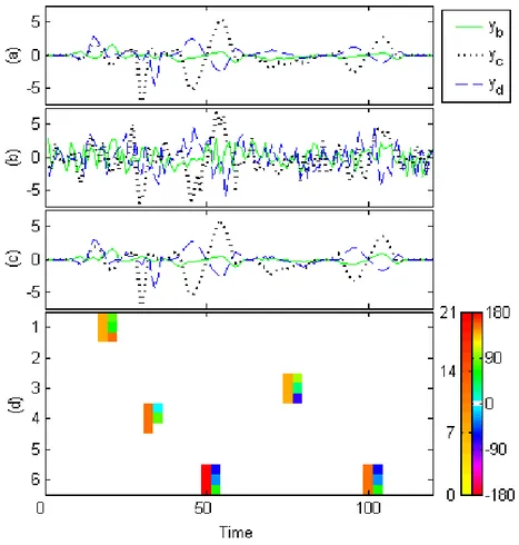
First, the quaternionic signal y∈ HN is formed using Eq. (11), which is plotted in
Fig. 1a. The first imaginary part yb is plotted as the solid green line, the second,
yc, as the dotted black line, and the third, yd, as the dashed blue line. Then, white
Gaussian noise is added, giving the noised signal ynthat is now characterized by an
RSB of 0 dB. This is shown in Fig. 1b, maintaining the the line style convention. Then, we deconvolute this signal yn through the dictionaryΨ using Q-OMP with
K=5 iterations. The denoised signal ˆyn, that is obtained by computing the K-sparse
approximation of yn, is plotted in Fig. 1c. The coding coefficients xl,τare the result
of the deconvolution, and they are shown in Fig. 1d, using the spikegram introduced in Section 4.2.
Fig. 1 Original (a), noised (b) and approximated (c) quaternionic signals (first imaginary part yb
as the solid green line; the second, yc, as the dotted black line; and the third, yd, as the dashed blue
We observe that Q-OMP recovers the generated coefficients well, and the approx-imation ˆynis close to the original signal y; the rMSE is only 2.8 %. This experiment
is randomly repeated 100 times, and the averaged rMSE is 4.7%. This illustrates the Q-OMP efficiency for denoising and deconvolution. In Fig. 1d, note that coeffi-cients x6,50and x6,100are coded with different amplitudes, but with the similar unit
quaternion q.
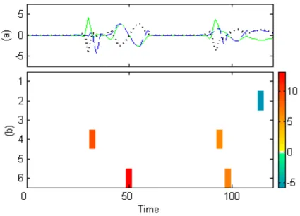
Q-OMP is now compared to M-OMP, only using the trivariate case. The pure quaternionic signal ynis now filled in a trivariate real signal yn∈RN×3as well as the
kernel dictionary. The M-OMP is applied with K= 5 iterations, and this gives the denoised signal ˆy
nthat is plotted in Fig. 2a. The rMSE is 81.7%, and the average
over 100 experiments is 76.8%. The associated spikegram is shown in Fig. 2b, us-ing the original visualization. We observe that the strong coefficients are relatively well recovered, although the others are not (temporal shift τ, kernel index l, and amplitude). However, although the strongest coefficients are recognized, this is not sufficient to obtain a satisfactory approximation. Indeed, multivariate sparse approx-imation is not adapted to this case, as it cannot take into account the cross-terms of the quaternionic vectorial part.
Fig. 2 Approximated trivariate real signal ˆy
n(a) and its associated spikegram (b).
A full quaternionic signal y∈ HN giving a quadrivariate real signal y∈ RN×4 is
now considered. If the coefficients are strictly real, the two methods are equivalent. If not, the Q-OMP performs better, although for the complexity, the quadrivariate correlation only has 4 terms, whereas the quaternionic one has 16.
6 Conclusion
We have presented here a new tool for sparse approximation with quaternions: the Q-OMP, a quaternionic extension of the OMP. This processes a right-multiplication linear combination of quaternionic signals. We have also presented a new spikegram visualization for the quaternionic coefficients. For the validation, the Q-OMP was applied to deconvolute simulation data, and is compared to the M-OMP.
The potential uses of Q-OMP include quaternionic signal processing such as deconvolution, denoising, variable selection, dimensionality reduction, dictionary learning, and all of the other classical applications that are based on sparsity. Prospects are to present the left-multiplication Q-OMP.
Acknowledgements The authors thank N. Le Bihan from GIPSA-DIS and Prof. S. Sangwine from University of Essex for their precious advises about quaternions.
Appendix
The MSE objective function is J= kεk22= εHε. The derivation of J with respect to
xis computed below.
To not lengthen the paper, calculus stages are not completely detailed. ∂ J ∂ x= ∂ J ∂ xa + ∂ J ∂ xb i+ ∂ J ∂ xc j+ ∂ J ∂ xd k =∂ ε H ∂ xa ε + εH∂ ε ∂ xa +∂ ε H ∂ xb εi + εH∂ ε ∂ xb i+∂ ε H ∂ xc ε j + εH∂ ε ∂ xc j+∂ ε H ∂ xd εk + εH∂ ε ∂ xd k. (13) Developing all the terms ofε = y − φ x and εH= yH− x∗φH
, we obtain: ∂ ε/∂ xa= −(φa+ φbi+ φcj+ φdk) = −φ ∂ εH/∂ xa= −(φaT− φ T bi− φ T c j− φ T dk) = −φ H ∂ ε/∂ xb= −(−φb+ φai+ φdj− φck) ∂ εH/∂ xb= −(−φbT− φ T ai− φ T dj+ φ T ck) ∂ ε/∂ xc= −(−φc− φdi+ φaj+ φbk) ∂ εH/∂ xc= −(−φcT+ φdTi− φ T aj− φbTk) ∂ ε/∂ xd= −(−φd+ φci− φbj+ φak) ∂ εH/∂ xd= −(−φdT− φcTi+ φbTj− φaTk).
Replacing these eight terms in Eq. (13), we have: ∂ J ∂ x = −φ H ε − εHφ −(−φT b− φaTi− φdTj+ φcTk)(−εb+ εai+ εdj− εck) (14) −εH(−φ a− φbi− φcj− φdk) −(−φT c + φdTi− φaTj− φbTk)(−εc− εdi+ εaj+ εbk) (15) −εH(−φ a− φbi− φcj− φdk) −(−φdT− φ T ci+ φ T bj− φ T ak)(−εd+ εci− εbj+ εak) (16) −εH(−φ a− φbi− φcj− φdk) = −φHε + 2εHφ + (14) + (15) + (16). (17)
Developing the three terms (14), (15) and (16), adding and factorizing, we obtain: (14) + (15) + (16) = −φHε − 2εHφ .
(18) With Eq. (17), we finally have:
∂ J ∂ x = −φ H ε + 2εHφ − φHε − 2εHφ = −2φHε = −2 hε, φ i . (19)
Thus, we can conclude that the atom which produces the strongest decrease of the MSEkεk22is the most correlated to the residue, as in the complex case.
Remark that this quaternion derivation has been done with the sum of compo-nentwise gradients. It is called pseudogradient by Mandic et al. who propose a quaternion gradient operator in [7]. Using these new derivative rules, we obtain ∂ J/∂ x∗= −φHε + 1/2 εHφ . However, maximizing this expression does not give
the optimal atom. It does not allow to recover known atoms in a simulated signal.
References
1. Q. Barth´elemy, A. Larue, A. Mayoue, D. Mercier, and J.I. Mars. Shift & 2D rotation invariant sparse coding for multivariate signals. IEEE Trans. on Signal Processing, 60:1597–1611, 2012.
2. S.F. Cotter, R. Adler, R.D. Rao, and K. Kreutz-Delgado. Forward sequential algorithms for best basis selection. Proc. IEEE Vision, Image and Signal Processing, 146:235–244, 1999. 3. G. Davis, S. Mallat, and Z. Zhang. Adaptive time-frequency decompositions with matching
pursuits. Optical Engineering, 33:2183–2191, 1994.
4. A.J. Hanson. Visualizing quaternions. Morgan-Kaufmann/Elsevier, 2006.
5. S. Javidi, C.C. Took, C. Jahanchahi, N. Le Bihan, and D.P. Mandic. Blind extraction of im-proper quaternion sources. In Proc. IEEE Int. Conf. Acoustics, Speech and Signal Processing ICASSP ’11, 2011.
6. S.G. Mallat and Z. Zhang. Matching pursuits with time-frequency dictionaries. IEEE Trans. on Signal Processing, 41:3397–3415, 1993.
7. D.P. Mandic, C. Jahanchahi, and C.C. Took. A quaternion gradient operator and its applica-tions. IEEE Signal Processing Letters, 18(1):47–50, 2011.
8. C.E. Moxey, S.J. Sangwine, and T.A. Ell. Hypercomplex correlation techniques for vector images. IEEE Trans. on Signal Processing, 51:1941–1953, 2003.
9. Y.C. Pati, R. Rezaiifar, and P.S. Krishnaprasad. Orthogonal Matching Pursuit: recursive func-tion approximafunc-tion with applicafunc-tions to wavelet decomposifunc-tion. In Proc. Asilomar Conf. on Signals, Systems and Comput., 1993.
10. E. Smith and M.S. Lewicki. Efficient coding of time-relative structure using spikes. Neural Comput., 17:19–45, 2005.
11. C.C. Took and D.P. Mandic. Quaternion-valued stochastic gradient-based adaptive IIR filter-ing. IEEE Trans. on Signal Processing, 58:3895–3901, 2010.
12. J.A. Tropp and S.J. Wright. Computational methods for sparse solution of linear inverse problems. Proc. of the IEEE, 98:948–958, 2010.
13. J. Via, D.P. Palomar, L. Vielva, and I. Santamaria. Quaternion ICA from second-order statis-tics. IEEE Trans. on Signal Processing, 59:1586–1600, 2011.