HAL Id: hal-00818815
https://hal.archives-ouvertes.fr/hal-00818815
Submitted on 29 Apr 2013
HAL is a multi-disciplinary open access
archive for the deposit and dissemination of
sci-entific research documents, whether they are
pub-lished or not. The documents may come from
teaching and research institutions in France or
abroad, or from public or private research centers.
L’archive ouverte pluridisciplinaire HAL, est
destinée au dépôt et à la diffusion de documents
scientifiques de niveau recherche, publiés ou non,
émanant des établissements d’enseignement et de
recherche français ou étrangers, des laboratoires
publics ou privés.
Graph-based inter-subject classification of local fMRI
patterns
Sylvain Takerkart, Guillaume Auzias, Bertrand Thirion, Daniele Schön, Liva
Ralaivola
To cite this version:
Sylvain Takerkart, Guillaume Auzias, Bertrand Thirion, Daniele Schön, Liva Ralaivola. Graph-based
inter-subject classification of local fMRI patterns. Third International Workshop Machine Learning
in Medical Imaging - MLMI 2012 (Held in Conjunction with MICCAI 2012), Oct 2012, Nice, France.
pp 184-192, �10.1007/978-3-642-35428-1_23�. �hal-00818815�
fMRI patterns
Sylvain Takerkart1,2, Guillaume Auzias3,1, Bertrand Thirion4, Daniele Sch¨on5,
and Liva Ralaivola2 1
CNRS, INT (UMR 7289), Marseille, France
2
Aix-Marseille University, LIF (UMR 7189), Marseille, France
3
CNRS, LSIS (UMR 7296), Marseille, France
4
INRIA-Saclay-Ile-de-France, Parietal team, Palaiseau, France
5
CNRS, INS (UMR 1106), Marseille, France
Abstract. Classification of medical images in multi-subjects settings is a difficult challenge due to the variability that exists between individ-uals. Here we introduce a new graph-based framework designed to deal with inter-subject functional variability present in fMRI data. A graph-ical model is constructed to encode the functional, geometric and struc-tural properties of local activation patterns. We then design a specific graph kernel, allowing to conduct SVM classification in graph space. Ex-periments conducted in an inter-subject classification task of patterns recorded in the auditory cortex show that it is the only approach to per-form above chance level, among a wide range of tested methods. Keywords: fMRI, classification, graphs, kernels, inter-subject, variabil-ity
1
Introduction
Since brain functions are considered to arise from activities distributed across networks, multivariate pattern recognition methods are adapted to study infor-mation processing in the brain. Multi-voxel pattern analysis (MVPA) of func-tional MRI allows to study the organization of distributed representations in the brain by using a classification framework where one attempts to predict the category of the input stimuli from the data [8]. MVPA has been largely applied within individual subjects [13].
However, because of the challenge posed by the large inter-individual vari-ability, very few studies describe inter-subject decoding, i.e successfull prediction on data from a subject that was not part of the training set. Among these, most rely on global (i.e full-brain) analysis, using large-scale features ([12], [15]). The few studying fine-scale local patterns achieve very low inter-subject general-ization performances [3], or use implicit abstract models [9]. None attempt to characterize the inter-subject functional variability (i.e the fact that the corre-lation between cortical folding and the underlying functional organization vary between subjects [4]) and use such characterization in the classification process.
2 S. Takerkart, G. Auzias, B. Thirion, D. Sch¨on, L. Ralaivola
In this paper, we introduce a new framework specifically aimed at tackling the challenges offered by inter-subject functional variability by modelling its spa-tial properties. Our approach integrates the fact that the geometric properties of local functional features, as well as their levels of activation, can vary across subjects, under the assumption that the underlying spatial structure of the local activation pattern is consistent. We therefore design a graphical model to rep-resent such patterns with their properties of interest: the nodes of the graphs represent small activation patches; their attributes carry the relevant features, such as their position and activation level; the edges of the graph (given by spa-tial adjacency) encode the spaspa-tial structure of the pattern. The classification is then performed directly in graph-space with Support Vector Machines (SVM), using a graph kernel specifically designed to take into account all properties of our graphical model. Since the topographic organization of primary sensory ar-eas ensures the structural consistency of activation patterns across subjects, we validate our framework on fMRI data recorded in the primary auditory cortex during a tonotopy experiment [10].
This paper is organized as follows: we detail the construction of our graphical model in section 2 and the kernel design in section 3; we then describe our experiments in section 4 and present our results in section 5.
2
Graphical Model of Activation Patterns
We here describe the design of a graphical model that summarizes the infor-mation relevant to characterize a pattern a pattern of activation measured with fMRI within a contiguous region of interest (ROI).
Graph nodes. Assuming that the ROI admits an underlying subdivision into a set of smaller and functionally relevant sub-regions, the first step to construct our graphical model estimates a parcellation of the ROI, i.e. a partition into a set of sub-regions or parcels [5]. Specifically, for a contiguous ROI R, we compute the parcellation V = {Vi}qi=1 of R, so that the q parcels verify: ∪
q
i=1Vi = R
and Vi∩ Vj = ∅ whenever i 6= j. We use V as the set of vertices of our graphical
model, each parcel corresponding to a node of the graph.
Nodes attributes: functional features. Let f be the real-valued function de-scribing the Bold activation. In a parcel Vi, the activations values {f (v)}v∈Vi
are summarized to form an n-dimensional feature vector F (Vi); we note F the
n× q matrix F = [F (V1) · · · F (Vq)] of functional features, where each column i
of F is F (Vi). A simple example of such F , which we make use of later on, is to
compute the mean activation value within a parcel.
Nodes attributes: geometric features. Let x be a coordinate system defined in R. We summarize the geometric information of parcel Vi through a
m-dimensional feature vector X(Vi) , computed from the locations {x(v)}v∈Vi.
We note X the m × q matrix X = [X(V1) · · · X(Vq)] of geometric features. X
may contain information on the shape or location of the parcels.
Graph edges: structural information. The set of edges is represented by a binary adjacency matrix A = (aij) ∈ Rq×q, where aij = 1 if parcels Vi and Vj
are spatially adjacent (i.e if ∃vi ∈ Vi,∃vj∈ Vjso that viand vjare neighbors, for
a given neighborhood definition), and aij= 0 otherwise. This adjacency matrix
encodes the spatial structure of the activation pattern.
Full graphical model. Using these definitions, we have defined an attributed region adjacency graph [14] (hereafter noted a-RAG) G = (V, A, F, X ), which represents the fMRI activation pattern within the ROI R by encoding functional, geometric and structural information.
3
Kernel design
The fully generic family of convolution kernels [7] is defined as: K(G, H) = X
g⊆G,h⊆H
Y
t
kt(g, h), (1)
where t ∈ N∗ is the, usually small, number of base kernels k
t, which act on
subgraphs g and h. To design a kernel for our a-RAGs, we need to choose the type of subgraphs, the value of t and to instantiate each base kernel kt.
Subgraphs used to design such kernels include paths and random walks [6], tree motives [11] etc. For simplicity reasons, we will here use paths of length two; note that the definitions below are directly extendable to other choices. Given the characteristics of the a-RAGs, we need to define t = 3 elementary kernels kf,
kg and ks, respectively acting on functional, geometric and structural features.
Let G = (VG, AG,FG,XG) and H = (VH, AH,FH,XH) be two a-RAGs: we
note gij = {i, j} and hkl = {k, l} two pairs of nodes in G and H, respectively;
let qG and qH be the number of nodes in G and H, respectively — note that qG
and qH may be different.
Functional kernel. Kernel kf aims at measuring the similarity of the
activa-tion in parcels of gij and hkl. We therefore propose the following product (and
thus positive definite) kernel kf(gij, hkl) = e−kF G i −F H kk2/2σf2· e−kF G j −F H l k2/2σ2f, (2)
where σf ∈ R∗+ and FpG (resp. FpH) is the pth column of FG (resp. FH).
Us-ing such a product of Gaussian kernels allows dealUs-ing with the inter-subject functional variability.
Geometric kernel. The second base kernel kg acts on the geometric features.
To allow for inter-subject variability, we follow the same principle as for the functional kernel, which gives:
kg(gij, hkl) = e−kX G i −X H kk2/2σg2· e−kX G j −X H l k2/2σg2, (3)
where σg∈ R∗+, and XpG (resp. XpH) is the pth column of XG (resp. XH).
Structural kernel. The base kernel ksaims at valuing the structural
similar-ity of G and H. Since our main hypothesis is that the structure is consistent across patterns recorded in different subjects, we adopt a decision function (by
4 S. Takerkart, G. Auzias, B. Thirion, D. Sch¨on, L. Ralaivola
opposition to the smooth functional and geometric kernels), by using the linear kernel on binary entries aG
ijand aHkl of the adjacency matrices AGand AH, which
encodes the fact that pairs gij and hkl are both edges:
ks(gij, hkl) = aGij.aHkl (4)
Resulting kernel. With the definitions of kf, kg and ks, we may define the
resulting kernel (with parameters σgand σf):
K(G, H) = qG X i,j=1 qH X k,l=1 kg(gij, hkl) · kf(gij, hkl) · ks(gij, hkl), (5)
Fig. 1.Graph construction process. A. Inflated cortical surface of the right hemisphere for one subject; Heschl’s gyrus is highlighted. B. A normalized activation pattern C. The two coordinates fields computed within the ROI. D. Example of parcellation with 10 parcels (arbitrary colors for illustration only). E. Example of an attributed graph: the nodes are located at the barycenter of the parcels and the color encodes the average level of activation in the parcel.
4
Real experiment and data analysis
fMRI tonotopy experiment. In order to test this framework, we used a dataset that was acquired to study the tonotopic property of the human auditory cortex. This property states that neighboring neurons in the cortex respond to auditory stimuli of neighboring frequencies. This results in a spatially organized mapping of the auditory cortex. Typically higher frequencies are represented in the medial part of the primary auditory cortex (A1) while lower frequencies are represented more laterally, although recent high resolution studies suggest a more complex patterns with mirror-symmetric frequency gradients [10].
For each of the nine subjects, a T1 image was acquired (1mm isotropic vox-els). Each stimulus consisted of a 8s sequence of 60 isochronous tones covering a narrow bandwidth around a central frequency f . There were five types of sequences (i.e. conditions), each one centered around a different frequency f (f ∈ {300Hz, 500Hz, 1100Hz, 2200Hz, 4000Hz}), with no overlap between the bandwidths covered by any two types of stimuli. Five functional sessions were
acquired, each containing six sequences per condition presented in a pseudo-random order. Echo-planar images (EPI) were acquired with slices parallel to the sylvian fissure (repetition time=2.4s, voxel size=2x2x3mm, matrix size 128x128). Fieldmaps were recorded to allow EPI geometric distortion correction.
Data processing and classification. The preprocessing of the functional data, carried on in SPM8 (www.fil.ion.ucl.ac.uk/spm), consisted in realignment, slice timing correction and “fieldmap” unwarping. Then, a generalized linear model was performed (in nipy: nipy.sourceforge.net) with one regressor of interest per stimulus. The weight (beta) maps of these regressors served as estimates of the response size for each stimulus. For the spatial proximity to have an anatomical meaning, one has to work on the 2D cortical surface. We therefore used freesurfer (surfer.nmr.mgh.harvard.edu) to extract the corti-cal surface from the T1 image and automaticorti-cally define the primary auditory cortex (Fig. 1A) as part of Heschl’s gyrus (thus defining our cortical ROI R in each subject). The beta maps are then projected onto the cortex, and slightly smoothed (equivalent fwhm of 3mm) in cortical space, which defines the func-tion {f (v)}v∈R (Fig. 1B). A 2D local coordinates system is defined through
a conformal mapping of R onto a rectangle [1], defining {x(v)}v∈R (Fig. 1C).
One then need a parcellation technique that produces homogeneous parcels. We use Ward’s hierarchical clustering algorithm on anatomo-functional features {f (v), x(v)}, with an added spatial constraint: the merging criterion of two adja-cent parcels consists in minimzing the variance across all parcels [12] (Fig. 1D), and the neighboring criterion is given by the neighboring of the vertices of the cortical mesh. Finally, we define one functional feature F , the mean activation in a parcel (normalized between 0 and 1) and a 2D geometric feature vector X as the coordinates of the barycenter of each parcel.
Using the kernel trick, one can then directly perform Support Vector Clas-sification in graph space (G-SVC) to guess the class of the input stimulus (i.e the tone frequency) from a given activation pattern. In practice, the Gram ma-trix was computed with custom-designed code, and given as input to the SVC function of the scikit-learn python module (scikit-learn.org), which uses Lib-SVM (www.csie.ntu.edu.tw/~cjlin/libsvm/) to implement Lib-SVM. A leave-one-subject-out cross-validation scheme was used to measure the classification accuracy. For each fold of this cross-validation, we estimated the kernel param-eters σf and σg as the median euclidean distance between the functional and
geometric (respectively) feature vectors of the parcels between all nodes of all example-graphs in the training set, which corresponds to a standard heuristic [2]. Two types of analyses were conducted. First, we performed simulations with a fixed number of nodes q for all graphs and all subjects; several simulations were conducted, with q ∈ {5, 6, 7, 8, 9, 10, 15, 20, 25, 30}. Second, we imposed different number of nodes for each subject, randomly taken in three intervals Iq = [5, 13],
[14, 22] and [5, 21]; for each of these intervals, we ran 18 simulations with different random sets of node numbers (each time with a different q for each subject).
In order to compare the performances of our framework to vector-based meth-ods, one need to define a vertex to vertex correspondance across subjects (which
6 S. Takerkart, G. Auzias, B. Thirion, D. Sch¨on, L. Ralaivola
is not needed with our framework). We therefore aligned the anatomy of all subjects to a standard spherical cortical space using freesurfer and projected the beta maps to this standard space. R is now common to all subjects and we can use {f (v)}v∈R as a feature set. Several classification algorithms were
then used, each time with several values of their respective hyper-parameters: 1) linear SVC; 2) non linear SVC, with gaussian (with σ ∈ {10−n}
n∈{−2,−1,0,1})
and polynomial (of order n ∈ {2, 3, 4}) kernels; 3) k-nearest neigbors (with k ∈ {3, 5, 7, 11, 15}); 4) logistic regression with l1 and l2 regularization (with
weight λ ∈ {10n}
n∈{2,3,4}).
5
Results and discussion
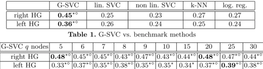
Table 1 contains the performances of our G-SVC framework vs. the different benchmark vector-based methods. The scores are the mean classification accu-racies across all folds of the cross-validation; for the benchmark methods, the reported score is the highest one across simulations ran with all values of their hyper-parameters; for G-SVC, it is the mean performances across all values of q. All vector-based methods performed similarly, but none of them performed sig-nificantely above chance level (equal to 0.2 since there were five types of auditory stimuli). Our G-SVC framework was the only method to perform significantely above chance level (one sample t-test, p < 0.05, indicated by a ⋆), in both the left and right Heschl’s gyri (HG). It also performed significantely better than the best benchmark method (linear SVC for the right HG, logistic regression for the left HG; paired t-test with matched left-out subject, p < 0.05; indicated by a ⋄). Table 2 describes the accuracy of our G-SVC depending on the number of graph nodes q. Our framework performed above chance level in all cases (one sample t-test, p < 0.05; ⋆), and significantely better than the best benchmark method (paired t-test, p < 0.05; ⋄) in all but two cases (left HG, q = 10, 15).
G-SVC lin. SVC non lin. SVC k-NN log. reg. right HG 0.45⋆⋄ 0.25 0.23 0.27 0.27
left HG 0.36⋆⋄ 0.26 0.24 0.25 0.24
Table 1.G-SVC vs. benchmark methods
G-SVC q nodes 5 6 7 8 9 10 15 20 25 30 right HG 0.48⋆⋄ 0.45⋆⋄ 0.45⋆⋄ 0.43⋆⋄0.47⋆⋄0.43⋆⋄0.44⋆⋄
0.48⋆⋄ 0.47⋆⋄ 0.44⋆⋄
left HG 0.33⋆⋄ 0.37⋆⋄ 0.35⋆⋄ 0.38⋆⋄0.35⋆⋄ 0.35⋆ 0.34⋆ 0.37⋆⋄
0.39⋆⋄ 0.38⋆⋄
Table 2.Influence of the number of graph nodes q in G-SVC
Results of the simulations using a randomized number of nodes q for each subject are given in Table 3. In all 108 simulations, our G-SVC framework per-formed above chance level (one sample t-test, p < 0.05, ⋆). This shows that the proposed kernel is efficient for graphs having different number of nodes. More-over, in 80% of the simulations (86/108), it outperformed the best benchmark method (paired t-test, p < 0.05, ⋄). Overall, the performances are very similar to the ones obtained when the number of nodes is fixed for all subjects.
Interval Iq [5,13] [14,22] [5,21] right HG 0.43 (18⋆, 18⋄ ) 0.45 (18⋆, 18⋄ ) 0.45 (18⋆, 18⋄ ) left HG 0.35 (18⋆, 12⋄ ) 0.36 (18⋆, 9⋄ ) 0.36 (18⋆, 11⋄ )
Table 3.Mean G-SVC performances with variable q over 18 simulations (number that resulted in accuracy above chance level ⋆, above the best benchmark method ⋄)
Discussion. In this paper, we designed a graphical model and a graph-kernel that allows to compare and discriminate high dimensional patterns of fMRI acti-vation across subjects. To our knowledge, this is the first time that a graph-based pattern recognition approach is used to study local fMRI activation patterns. Specifically, we have demonstrated the power of this approach in a classification task that aims at predicting experimental variables from fMRI patterns when the classifier is trained on data from a set of subjects and its generalization performance is tested on data from a different subject.
Our G-SVC framework performed above chance level in all cases, whereas none of the benchmark methods did. This validates that this framework is ap-propriate to deal with inter-subject variability that is not accounted for by a state of the art group alignment, such as the one offered in freesurfer. How-ever, it is important to use the anatomical information at our disposal, as was attempted in this study by i) working on the cortical surface, and ii) defining a local coordinates system within our region of interest for each subject, thus using the most of the local individual anatomy. Indeed, we also tested G-SVC using the raw three-dimensional voxel coordinates for x, and the performances (not reported here) were systematically lower.
A major asset of using a graph kernel such as the one defined here is that the graphs can have different number of nodes, without having to strictly solve a graph matching problem, i.e to assign nodes to one another across instances. This is emphasized by the results of our simulations where the number of nodes was randomly chosen and forced to be different for each subject. In those, our framework still outperformed vector-based methods, demonstrating the ability to deal with graphs with different node numbers. We also noted a few simulations where the classification accuracy was higher than with a fixed q for all subjects. This suggests that there might exist an “optimal” number of nodes for each subject and that performances could increase by adequately choosing q for each subject. We will address this in future work, for instance by using a model selection criterion (BIC, AIC etc.) in the parcellation. Another source of potential improvement lies in selecting the hyper-parameter σf and σg of the kernel in a
nested cross-validation, rather than using a heuristic estimator.
6
Conclusion
We have designed a graphical model carrying functional, geometric, and struc-tural features to represent spatial patterns. With a custom-designed graph kernel providing a natural metric, this framework seems particularly attractive to per-form classification tasks in multi-subject settings, as evidenced by the conclusive results obtained here when dealing with inter-subject functional variability in
8 S. Takerkart, G. Auzias, B. Thirion, D. Sch¨on, L. Ralaivola
fMRI data. This modelling strategy therefore opens the possibility to character-ize and discriminate populations based on their functional patterns of activation.
7
Acknowledgment
Thanks to the CNRS Neuro-IC program for funding, and to the Centre IRMf de Marseille and its staff for data acquisition.
References
1. G. Auzias, J. Lef`evre, A. Le Troter, C. Fischer, M. Perrot, J. R´egis, and O. Coulon. Model-driven harmonic parameterization of the cortical surface. In Proc. 14th MICCAI, LNCS 6892 (Part II), pages 310–317, Toronto, Canada, Sep. 2011. 2. B. Caputo, K. Sim, F. Furesjo, and A. Smola. Appearance-based object recognition
using svms: which kernel should i use? In Proc. of NIPS workshop on Stat. methods for computational experiments in visual processing and computer vision, 2002. 3. J. A. Clithero, D. V. Smith, R. M. Carter, and S. A. Huettel. Within- and
cross-participant classifiers reveal different neural coding of information. NeuroImage, 56(2):699 – 708, 2011. Multivariate Decoding and Brain Reading.
4. D. C. Van Essen and D. L. Dierker. Surface-Based and probabilistic atlases of primate cerebral cortex. Neuron, 56(2):209–225, October 2007.
5. G. Flandin, F. Kherif, X. Pennec, G. Malandain, N. Ayache, and J.-B. Poline. Improved detection sensitivity of functional MRI data using a brain parcellation technique. In Proc. 5th MICCAI, LNCS 2488 (Part I), pages 467–474, 2002. 6. T. G¨artner. Exponential and geometric kernels for graphs. In NIPS Workshop on
Unreal Data: Principles of Modeling Nonvectorial Data, 2002.
7. D. Haussler. Convolution kernels on discrete structures. Technical Report UCSC-CRL-99-10, UC Santa Cruz, 1999.
8. J. V. Haxby, M. I. Gobbini, M. L. Furey, A. Ishai, J. L. Schouten, and P. Pietrini. Distributed and overlapping representations of faces and objects in ventral tempo-ral cortex. Science, 293(5539):2425–2430, 2001.
9. J. V. Haxby, J. S. Guntupalli, A. C. Connolly, Y. O. Halchenko, B. R. Conroy, M. I. Gobbini, M. Hanke, and P. J. Ramadge. A common, High-Dimensional model of the representational space in human ventral temporal cortex. Neuron, 72(2):404–416, October 2011.
10. C. Humphries, E. Liebenthal, and J. R. Binder. Tonotopic organization of human auditory cortex. NeuroImage, 50(3):1202 – 1211, 2010.
11. P. Mah´e and J. P. Vert. Graph kernels based on tree patterns for molecules. Machine Learning, 75:3–35, 2009.
12. V. Michel, A. Gramfort, G. Varoquaux, E. Eger, C. Keribin, and B. Thirion. A supervised clustering approach for fMRI-based inference of brain states. Pattern Recognition, 45(6):2041 – 2049, 2012.
13. K. A. Norman, S. M. Polyn, G. J. Detre, and J. V. Haxby. Beyond mind-reading: multi-voxel pattern analysis of fMRI data. Trends in cognitive sciences, 10(9):424– 430, 2006.
14. T. Pavlidis. Structural pattern recognition. Springer-Verlag, 1977.
15. R. A. Poldrack, Y. O. Halchenko, and S. J. Hanson. Decoding the Large-Scale structure of brain function by classifying mental states across individuals. Psycho-logical Science, 20(11):1364–1372, November 2009.