Measurement of morphological modifications of cell population using lensless imaging.

HAL Id: tel-01169363

https://tel.archives-ouvertes.fr/tel-01169363

Submitted on 29 Jun 2015

HAL is a multi-disciplinary open access

archive for the deposit and dissemination of sci-entific research documents, whether they are pub-lished or not. The documents may come from teaching and research institutions in France or abroad, or from public or private research centers.

L’archive ouverte pluridisciplinaire HAL, est destinée au dépôt et à la diffusion de documents scientifiques de niveau recherche, publiés ou non, émanant des établissements d’enseignement et de recherche français ou étrangers, des laboratoires publics ou privés.

Measurement of morphological modifications of cell

population using lensless imaging.

Srikanth Vinjimore Kesavan

To cite this version:

Srikanth Vinjimore Kesavan. Measurement of morphological modifications of cell population using lensless imaging.. Other [cond-mat.other]. Université de Cergy Pontoise, 2014. English. �NNT : 2014CERG0732�. �tel-01169363�

CELL CULTURE MONITORING BY MEANS OF

LENSFREE VIDEO MICROSCOPY

SUIVI DE CULTURE CELLULAIRE PAR

IMAGERIE SANS LENTILLE

Thesis for the degree of Doctor of Philosophy

Etablissement d'inscription: UNIVERSITE CERGY-PONTOISE

Ecole doctorale: ED SI - Sciences et Ingénierie

Spécialité: Physique – Cergy

Submitted by Srikanth VINJIMORE KESAVAN

Prepared in the laboratory of

Laboratoire Imagerie et Systèmes d'Acquisition (LISA), CEA, Grenoble

Jury Members:

Dr. Cédric ALLIER (PhD Supervisor)

Commissariat à l'Energie Atomique et aux Energies Alternatives, France

Dr. Bernard CHALMOND (PhD Director)

Université de Cergy-Pontoise

CMLA, École normale supérieure de Cachan, France

Dr. Jean-Marc DINTEN (Chief of lab ‘LISA’ and Examinateur)

Commissariat à l'Energie Atomique et aux Energies Alternatives, France

Dr. Antoine DELON (Rapporteur)

Université Joseph Fourier, France

Dr. Manuel THERY (Rapporteur)

Commissariat à l'Energie Atomique et aux Energies Alternatives, France

Dr. Xavier GIDROL (Examinateur)

Commissariat à l'Energie Atomique et aux Energies Alternatives, France

Dr. Pierre ROCHETEAU (Examinateur)

Institut Pasteur, France

Dr. Spencer SHORTE (Examinateur)

ACKNOWLEDGEMENTS

From March 1, 2011, the day I started my master’s internship, until the end of my PhD, Cédric Allier has been an exceptional supervisor. He has always been there for friendly chats, for discussions, questions, suggestions, critical evaluation, motivation, and encouragement, while providing independence and freedom at the same time. He always stayed positive even during the initial stages when we contaminated the incubator and killed all the cells. He encouraged me irrespective of the outcome of the experiments. His passion for science and open-minded approach to learn new things has certainly had a positive impact on my PhD work. He has been the best mentor I have ever had and I have learnt a lot from him. I cannot express my gratitude enough to Cédric for being as exceptional as he had been for the past 3.5 years and certainly this acknowledgements section would not be enough. If I supervise a PhD student someday, I have a real-life experience of how a PhD supervisor should be.

I thank both Jean-Marc Dinten and Bernard Chalmond for being exceedingly considerate and supportive. They provided critical evaluation of the work, Jean-Marc from an ‘imaging’ point of view, and Bernard from ‘statistics’ point of view. They always appreciated the work, which motivated me to go further. The telephonic conferences with Bernard have always given me a fresh perspective on the results.

I looked forward to every day of my PhD. I never once felt stressed or pressured or exhausted, and this was mainly due to the support from Cédric, Jean-Marc, and Bernard.

Fabrice is the courageous researcher who gave me the incubator in his lab to test lensfree imaging system. He was so brave that even after the initial contamination that lensfree imaging caused, he gave us another chance. My first exposure to cell culture and cell biology was through Fabrice. He was very friendly and aside from very interesting discussions about cell biology, he also taught me important French and Spanish phrases that cannot be written here. But, I would definitely remember those phrases and would use them wisely. Discussions involving lensfree imaging have always been fascinating. For this, and for all the help that they offered during my PhD, I thank the ‘Lensfree team’ and all those who use lensfree system, including Thomas Bordy, Sophie Morel, Fabien Momey, Olivier Cioni, Lionel Herve, Jean-Guillaume Coutard, Samy Strola. I also thank Rolland Sauze for the software support and Henry Grateau for design and fabrication. My special thanks to Thomas from whom I learnt about fabrication of the system and instrumentation, and also to Fabien for all those image processing and data visualization techniques that he taught me. Fabien played a major role in the article that was published in Nature Scientific Reports, without his support, the article couldn’t have gotten its weightage and credibility. My wishes to Anthony Berdeu who joined the team recently.

I thank the entire lab of LISA (current lisa members and alumni), for its warmth and support especially Sophie Morel and Veronica Sorgato who gave me 40 cents for coffee, which gave me the motivation to stay late and finish the cell migration chapter of this PhD thesis. I thank Veronique Duvocelle, secretary of LISA, for being so helpful and kind, without her, the administrative processes would have been so very difficult. I thank Lionel and his wife for giving their house to host my ‘pot de marriage’.

The success of my PhD work is mainly because of our collaborators, which include, Fabrice Navarro, Mathilde Menneteau, Eric Sulpice, Xavier Gidrol, Delphine Freida, Nathalie Picollet, Monica Dolega, Fabien Abeille (who taught me cell culture techniques and collaborated with me for the PNIPAM project), Vincent Haguet, Patricia Obeid, our collaborators from Institut Pasteur, from Grenoble Institute of Neurosciences (Boudewijn

Vander Sanden, Charles Di Natale). My knowledge in biology comes from constant even stupid questions that I asked each one of them, to which they have responded with patience every single time.

I cannot express my gratitude enough to my parents, my grandparents, my sister and my wife, so I dedicate this PhD dissertation to them. My wife’s incredible support on the day of the defense allowed me to solely concentrate on my presentation, when she took care of all the rest. I also thank my ‘Atthai’ who tutored me during my school days.

Special thanks to all my friends, especially to my brother-in-law and my friend Mithun, and my friend Vinoth, who gave me support and breaks when I needed the most.

This PhD work was possible only because of the support from everyone that I mentioned here and also support from those that I might have missed to mention...

TABLE OF CONTENTS

ABSTRACT

………...………...………...I

ABBREVIATIONS

………...………...………...III

LIST OF FIGURES

………...………...………...IV

1 INTRODUCTION

………...………...………...1

2 DEVELOPMENT OF LENSFREE VIDEO MICROSCOPE

………...9

2.1 LENSFREE IMAGING

………...………...10

2.1.1 Principle………...………...10

2.1.2 Design and development………...………...11

2.2 LENSFREE IMAGING FOR CELL

………...………...15

2.3 LENSFREE VIDEO MICROSCOPE

………...………...16

2.3.1 Hardware considerations………...…………...17

2.3.2 Software – Holographic reconstruction………...………...24

2.3.2.1 Software – Holographic reconstruction of adherent cells

………...……….27

3 CELL CULTURE MONITORING

………...…...35

3A. MONITORING CELL-SUBSTRATE ADHESION AND CELL SPREADING

...37

3A.1 INTRODUCTION

….………...………....38

3A.2 RESULTS

….………...40

3A.2.1 Cell-substrate adhesion…...………40

3A.3 DISCUSSION

…...………...49

3A.4 METHODS

…...………...53

3B MONITORING CELL DIVISION AND DETERMINATION OF CELL

DIVISION ORIENTATION

…...……….60

3B. 1 INTRODUCTION

…....………...61

3B.2 RESULTS

…....………...63

3B.2. 1 Detection of dividing cells

………63

3B.2.2 Comparison with EdU proliferation assay…....………...67

3B.2.3 Inhibiting cell proliferation using ActinomycinD…....………..69

3B.2.4 Monitoring cell proliferation kinetics…....………...71

3B.2. 5 Application to Other Cell Types Including Primary Cells

…....………...73

3B.2. 6 Determination of cell division orientation…...………74

3B.3 DISCUSSION

…...………...76

3B.4 METHODS

…...………...80

3C MONITORING CELL DIFFERENTIATION

…....………...88

3C.1 INTRODUCTION

……….89

………92

3C.3 DISCUSSION

…...……….101

3C.4 METHODS

…...……….103

3D MONITORING CELL DEATH

…....………....107

3D.1 INTRODUCTION

….………....108

3D.2 RESULTS

…...………...110

3D.2.1 Cell death of U2OS cells…....………..112

3D.2.2 Cell death of human Mesenchymal Stem Cells (hMSCs)

…...……….116

3D.2.3 Other cell types and substrates…...………...120

3D.3 DISCUSSION

…...………122

3D.4 METHODS

…....……….123

3E CELL MIGRATION AND ITS ALTERATIONS

…....………..…127

3E.1 CELL MIGRATION ON 2D SUBSTRATES

…...………...129

3E.2 CELL MIGRATION ON 3D SUBSTRATES: Network formation between 3D acini structures

…...………...…...…...137

3E.3 EXPLORATORY MIGRATION: 3D/2D INTERFACE

………...143

3E.4 REVERSIBLE AND IRREVERSIBLE ALTERATION IN CELL MIGRATION

…....………. 144

3E.4.1 Cell migration and division…....………....145

3E.4.2 Cell migration and differentiation…...………..146

3E.4.3 Cell migration and death…...………...149

3E.4.4 Quiescence and cell migration…...……….153

4 CASE STUDIES

…...……….163

4.1 TEMPERATURE MEDIATED CELL DETACHMENT–USING PNIPAM GRAFTED SUBSTRATES

….………...165

4.1.1 Introduction…....………..165

4.1.2 Results…....……….167

4.1.3 Discussion…...……….170

4.1.4 Methods

…....………..172

4.2 3D CELL CULTURE: RWPE1 CELL POLARITY

…...………...175

4.2.1 Introduction…...……….175

4.2.2 Results………...176

4.2.3 Discussion

………...178

4.2.4 Methods…....………..179

4.3 3D CELL CULTURE: ENDOTHELIAL NETWORK FORMATION

…...………...180

4.3.1 Introduction………...180

4.3.2 Results…...………180

4.3.3 Discussion………...183

4.3.4 Methods…...……….184

4.4 NORMAL AND REDUCED TEMPERATURES IN NORMOXIC AND ANOXIC CONDITIONS

…...………....185

4.4.1 Introduction……….…...185

4.4.2 Results…....……….185

4.4.2.2 Myoblasts at 4°C, 0% 02

…...………190

4.4.3 Discussion…...……….192

5. CONCLUSION AND FUTURE PERSPECTIVES

…...………...196

I

ABSTRACT

Biological studies always start from curious observations. This is exemplified by description of cells for the first time by Robert Hooke in 1665, observed using his microscope. Since then the field of microscopy and cell biology grew hand in hand, with one field pushing the growth of the other and vice-versa. From basic description of cells in 1665, with parallel advancements in microscopy, we have travelled a long way to understand sub-cellular processes and molecular mechanisms. With each day, our understanding of cells increases and several questions are being posed and answered. Several high-resolution microscopic techniques are being introduced (PALM, STED, STORM, etc.) that push the resolution limit to few tens of nm, taking us to a new era where ‘seeing is believing’. Having said this, it is to be noted that the world of cells is vast, with information spread from nanometers to millimeters, and also over extended time-period, implying that not just one microscopic technique could acquire all the available information. The knowledge in the field of cell biology comes from a combination of imaging and quantifying techniques that complement one another.

Majority of modern-day microscopic techniques focuses on increasing resolution which, is achieved at the expense of cost, compactness, simplicity, and field of view. The substantial decrease in the field of observation limits the visibility to a few single cells at best. Therefore, despite our ability to peer through the cells using increasingly powerful optical instruments, fundamental biology questions remain unanswered at mesoscopic scales. A global view of cell population with significant statistics both in terms of space and time is necessary to understand the dynamics of cell biology, taking in to account the heterogeneity of the population and the cell-cell variability. Mesoscopic information is as important as microscopic information. Although the latter gains access to sub-cellular functions, it is the former that leads to high-throughput, label-free measurements. By focusing on simplicity, cost, feasibility, field of view,

II

and time-lapse in-incubator imaging, we developed ‘Lensfree Video Microscope’ based on digital in-line holography that is capable of providing a new perspective to cell culture monitoring by being able to capture the kinetics of thousands of cells simultaneously. In this thesis, we present our lensfree video microscope and its applications for in-vitro cell culture monitoring and quantification.

We validated the system by performing more than 20,000 hours of real-time imaging, in diverse conditions (e.g.: 37°C, 4°C, 0% O2, etc.) observing varied cell types and culture conditions (e.g.: primary cells, human stem cells, fibroblasts, endothelial cells, epithelial cells, 2D/3D cell culture, etc.). This permitted us to develop label-free cell based assays to study the major cellular events – cell adhesion and spreading, cell division, cell division orientation, cell migration, cell differentiation, network formation, and cell death. The results that we obtained respect the heterogeneity of the population, cell to cell variability (a raising concern in the biological community) and the massiveness of the population, whilst adhering to standard cell culture practices - a rare combination that is seldom attained by existing real-time monitoring methods.

We believe that our microscope and associated metrics would complement existing techniques by providing wide field of view with micrometric resolution.

III

ABBREVIATIONS

FOV Field of View ROI Region of Interest siRNA Small interfering RNA

ECIS Electric Cell Substrate Impedance Sensing CCD Charge-Coupled Device

CMOS Complementary Metal–Oxide–Semiconductor LED Light Emitting Diode

hMSC Human Mesenchymal Stem Cells PIV Particle Image Velocimetry BME β-mercaptoethanol

PNIPAM Poly(N-isopropylacrylamide)

LCST Lower Critical Solution Temperature ATRP Atom Transfer Radical Polymerization EMT Epithelial Mesenchymal Transition

IV

LIST OF FIGURES

CHAPTER 1

Figure 1.1 Standard lens-based time-lapse microscope

Figure 1.2 Schematic diagram of typical flow cytometer setup

Figure 1.3 Schematic diagram of Electric Cell Substrate Impedance Sensing CHAPTER 2

Figure 2.1.1 Principle of in-line holography introduced by Gabor. Figure 2.1.2 Digital in-line holography Setup used by Xu et al.

Figure 2.1.3 Lensless digital holographic microscope setup by Repetto et al. Figure 2.1.4 Modified lensfree imaging design using CMOS imaging sensor Figure 2.3.1 Lensfree video microscope prototypes

Figure 2.3.2 Temperature increase and frequency of imaging Figure 2.3.3 Parallel real-time imaging inside standard incubator

Figure 2.3.4 Different cell types in different conditions – imaged by lensfree video microscope.

Figure 2.3.5 Full FOV lensfree image

Figure 2.3.6 Schematic diagram explaining holographic reconstruction method 1 Figure 2.3.7 Schematic diagram explaining holographic reconstruction method 2 Figure 2.3.8 Holographic reconstruction

Figure 2.3.9 Comparison of reconstructed lensfree image and lens-based microscopic image

CHAPTER 3A

Figure 3A.1 Change in lensfree holographic pattern during cell-substrate adhesion Figure 3A.2 Discrimination of floating and adhering cells

Figure 3A.3 Floating and adherent cells imaged by lensfree and lens-based microscopes

V

Figure 3A.4 Cell-substrate adhesion kinetics of hMSCs and Primary human fibroblasts

Figure 3A.5 Quantification of cell-substrate adhesion and spreading Table 3A.6 Overview of different cell-substrate adhesion assays

Figure 3A.7 Cell-cell variability in cell-substrate adhesion and spreading Figure 3A.8 Age-dependent cell-substrate adhesion kinetics

Figure 3A.9 Pattern recognition of floating cells Figure 3A.10 Gray-level detection of adherent cells Table 3A.11 Validation of automated cell count

CHAPTER 3B

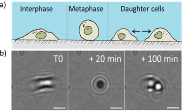
Figure 3B.1 Changes in cell shape and adhesion during cell division Figure 3B.2 Detection of dividing cells

Table 3B.3 Validation of automated detection of dividing cells Figure 3B.4 Comparison with standard EdU proliferation assay Figure 3B.5 Effect of ActinomycinD on cell proliferation

Table 3B.6 Effect of ActinomycinD on cell proliferation –EdU Proliferation assay Figure3B.7 Cell proliferation kinetics

Figure 3B.8 Kinetics of cell proliferation of different cell types. Figure 3B.9 Cell division orientation

Figure 3B.10 Unsuccessful cell division Figure 3B.11 Applicability to other cell types Figure 3B.12 Increased temporal resolution

Figure 3B.13 Automated detection of cell division orientation CHAPTER 3C

Figure 3C.1 Adipogenic differentiation and associated changes Figure 3C.2 Neuronal differentiation and associated changes

VI

Figure 3C.3 hMSC and differentiated adipocyte

Figure 3C.4 Adipogenic differentiation of single hMSC

Figure 3C.5 Gray-level based detection of differentiated and non-differentiated cells

Figure 3C.6 Comparison with standard lens-based microscopic images. Figure 3C.7 Reconstruction and segmentation of differentiated adipocytes. Figure 3C.8 Kinetics of adipogenic differentiation

Figure 3C.9 Different stages of adipogenic differentiation

Figure 3C.10 Time-lapse lens-based microscopic image of neuronal differentiation Figure 3C.11 Neuronal differentiation of a single hMSC

Figure 3C.12 Kinetics of neuronal differentiation

Figure 3C.13 Mesenchymal stem cell differentiation to other types CHAPTER 3D

Table 3D.1 Cell viability assays

Figure 3D.2 Cell death observed by lensfree video microscopy Figure 3D.3 Comparison with lens-based microscopy

Figure 3D.4 Cell death – human Osteo Sarcoma (U2OS) cells Figure 3D.5 Cell death –hMSCs

Figure 3D.6 Change in gray value during cell death of hMSCs Figure 3D.7 Cell death of DU145 and PC3 cells

Figure 3D.8 Cell death of NIH3T3 cells Figure 3D.9 Cell death on micro-patterns

CHAPTER 3E

Figure 3E.1 Random cell migration of NIH3T3 cells on 2D substrate

Figure 3E.2 Random cell migration of a single neuron cells on 2D substrate Figure 3E.3 Circular cell migration: RWPE1 cells on 2D substrate

VII

Figure 3E.4 Directed rectilinear cell migration of keratinocytes on 2D substrate Figure 3E.5 Directed migration on 2D substrate – Wound healing

Figure 3E.6 Cell velocity in relation to confluence Figure 3E.7 Cell migration at confluence – RPE1 cells. Figure 3E.8 Cell migration at confluence - hMSCs

Figure 3E.9 Velocity as a function of length of the cells, aspect-ratio of the cells, and adhesion of the cells.

Figure 3E.10 Directed migration on 3D –acini network formation. Figure 3E.11 Formation of network between 4 acini structures Figure 3E.12 Failed Connection

Figure 3E.13 Formation of network between 3acini structures Figure 3E.14 Multiple branching

Figure 3E.15 Close-gap branching Figure 3E.16 Trajectories

Figure 3E.17 Exploratory migration

Figure 3E.18 Cell migration and cell division

Figure 3E.19 Myoblasts cell migration during cell division

Figure 3E.20 Reduction in cell velocity during neuronal differentiation Figure 3E.21 Reduction in area of cell body during neuronal differentiation Figure 3E.22 Chronograph cell differentiation

Figure 3E.23 Cell migration and cell death - Fibroblasts Figure 3E.24 Cell migration and cell death - hMSCs Figure 3E.25 Cell size and cell adhesion during cell death Figure 3E.26 Chronograph – cell death

Figure 3E.27 Single migrating hMSC during cell death Figure 3E.28 Scratch assay

VIII

Figure 3E.29 Computational analysis Figure 3E.30 Wound area measurement

Figure 3E.31 Rate of wound healing at different temperatures CHAPTER 4

Figure 4.1.1 Time-taken to descend below LCST Figure 4.1.2 Percentage of cell detachment

Figure 4.1.3 Static contact angle variation with respect to temperature Figure 4.1.4 Loss of cell detachment efficiency

Figure 4.1.5 PNIPAM grafting procedure

Figure 4.1.6 Protocol schematic of a cell detachment experiment Figure 4.2.1 Lensfree imaging of 3D cell culture

Figure 4.2.2 Discriminating acini and spheroids from lensfree holographic patterns Figure 4.2.3 Growth of acini

Figure 4.3.1 HUVEC angiogenesis observed using lensfree video microscope Figure 4.3.2 Analysis of HUVEC angiogenesis

Figure 4.3.3 Analysis of the kinetics of HUVEC network Figure 4.4.1 Single fibers

Figure 4.4.2 Proliferation of satellite cells that exit from single fibers Figure 4.4.3 Myoblast trajectories

Figure 4.4.4 Cell migration of myoblast Figure 4.4.5 Cell migration of myoblast

Figure 4.4.6 Proliferation of myoblasts at 37°C Normoxia

Figure 4.4.7 Cell migration and cell shrinking of myoblasts at 4°C anoxia. Figure 4.4.8 Cell detachment of myoblasts at 4°C anoxia.

INTRODUCTION

1

1. INTRODUCTION

Imaging is an inherent part of biology. Microscope allows researchers to peer through cells and sub-cellular structures. Rapid advancements have occurred in the field of microscopy over the past decade and several super resolution microscopy techniques that break the diffraction barrier first stated by Abbe in 1873, have been reported (Betzig et al., 2006; Egner & Hell, 2005; Hell, 2007; Hess, Girirajan, & Mason, 2006; Rust, Bates, & Zhuang, 2006; Schermelleh, Heintzmann, & Leonhardt, 2010; Sengupta, Van Engelenburg, & Lippincott-Schwartz, 2012). Super-resolution techniques overcame, more precisely circumvented, the Abbe diffraction limit by using tailored illumination, nonlinear fluorophore responses, or by using single molecule localization (Schermelleh et al., 2010; Sengupta et al., 2012). Modern day microscopic techniques have reached spatial and lateral resolution close to few tens of nm, popularizing the phrase ‘Seeing is Believing’. However, increase in resolution is achieved at the expense of cost, compactness, simplicity and importantly field of view (FOV). Hence, despite increased resolution, to perform in-vitro quantification (e.g.: quantification of cell proliferation, etc.) flow cytometry is preferred over microscopy.

In-vitro quantification is about providing information about the status of the cells (quiescent, dying, proliferating, etc.). This is the preliminary step towards understanding complex cellular mechanisms, for example, to assess effectiveness of drugs, siRNAs, to control cell behavior, and to test the compatibility of materials. It is therefore an inevitable step well before in-vivo testing. Modern-day lens-based microscopes are not commonly used to perform in-vitro quantification mainly due to lack of (or difficulty in obtaining) spatial and temporal information.

INTRODUCTION

2

Spatial information or field of view (FOV) is often traded off for resolution. Typical FOV with 20X magnification can visualize few single cells at best. Even with a lower magnification of 10X, only few tens of cells (or couple of hundreds at best) are observed. Hence the global view, which is necessary to understand the entirety of the population, is lost. Temporal information, on the other hand, is lost due to the inability to perform real-time monitoring. This is because, cells cannot stay alive outside the incubator for extended period of time. The incubator provides ambient environmental conditions needed for the viability of cells (humidity, %02, %CO2, and temperature). Microscopes cannot be placed inside the standard incubator mainly due to their bulkiness, and elevated temperature and humidity inside the incubator. In order to observe the dynamics of cell culture, using lens-based microscopes, a personnel intervention is required at static time-points, which apart from being labor-intensive, raises concerns about sterility, and incapacity to follow same cell at single cell level. As a response, to perform continuous live-cell imaging, time-lapse microscopy was introduced. Lens-based time-lapse microscopes maintain suitable culture environment, by housing an environmental chamber (Fig. 1.1). As a consequence, the cost and bulkiness of the microscope is increased manifold times, along with the complexity in manipulating culture dishes during the experiment while the FOV remains restricted. Further, mostly standard video microscopes necessitate labeling for clear visualization and quantification. This raises concerns related to cytotoxicity, bias introduced by labeling (Marx, 2013), photo-toxicity, and photo-bleaching. These factors limit the use of standard video microscope for in-vitro quantification.

INTRODUCTION

3

Figure 1.1: Standard lens-based time-lapse microscope. Standard lens-based time-lapse microscope setup housing an environmental chamber connected to external CO2, O2 and temperature modules to provide ambient cell culture conditions.

(Courtesy: http://zeisscampus.magnet.fsu.edu/)

Therefore, researchers are forced to resort to marker-dependent flow cytometry assays, which monopolize in-vitro quantification. A flow cytometer performs automated quantification, and provides information about the state of the cell, depending on the uptake (or not) of expensive biomarkers, by the cells. The technique analyses entire cell populations and provides high-throughput information (Fig. 1.2). However, markers are indispensable for quantification using flow cytometry. Though several markers that do not affect the cells are being introduced, most of the currently used markers are cytotoxic and are also suspected to be introducing bias in measurements (Marx, 2013). Also, another major limitation with the technique is the need for the cell population to be harvested for end-point analysis. Therefore, in most cases, the cell population is lost, along with the continuity of quantification, rendering the assays invasive and non-continuous.

INTRODUCTION

4

The only way to perform continuous measurement using flow cytometry is by conducting several measurements at different time points using cultures that are subjected to same treatment. The end result is an extrapolation of data obtained from different time points. However, the data cannot be called continuous since the population is not the same.

Figure 1.2: Schematic diagram of typical flow cytometer setup. The fluidics system passes the cell population one-by-one through the laser. Based on light scattering, the uptake of markers (or not) by the cell is quantified. (Courtesy: www.abdserotec.com)

In order to overcome the limitations and to perform label-free, real-time continuous measurements, several techniques are being introduced. One of the well popularized techniques is ECIS – Electric Cell Substrate Impedance Sensing (Fig. 1.3). The technique takes advantage of the fact that the cell membranes are strong insulators. By measuring the substrate impedance changes, presence or absence of cells and also the surface area covered by cells are quantified. Using this information, the status of the cell culture is determined leading to several label-free assays (Arias, Perry, & Yang, 2010; Diemert et al., 2012; Hondroulis, Liu, & Li, 2010; Hong, Kandasamy, Marimuthu, Choi, & Kim, 2011; Michaelis, Wegener, & Robelek, 2013). Nevertheless, it is an indirect approach. First, the

INTRODUCTION

5

obtained parameters are surrogate measurements of substrate impedance changes. Second, the measurement is restricted to cell population and is not usually extended to the level of single cells. Third, the cells are not visualized which represents a huge loss of information in the era of HCA. Though various techniques that are being introduced, as alternatives provide higher resolution and feasibility, they face one or combination of the limitations mentioned above (Marrison, Räty, Marriott, & O’Toole, 2013).

Figure 1.3: Schematic diagram of Electric Cell Substrate Impedance Sensing. The setup comprises of gold electrode surfaces and culture wells built around the gold electrode surfaces. (Courtesy: www.biophysics.com)

INTRODUCTION

6

An apt alternative platform should combine the advantages of all the three major techniques (time-lapse microscopy, flow cytometry, ECIS) mentioned above. That is, the platform, (i) should be readily applicable to cell culture imaging inside standard incubator, (ii) should be able to provide label-free information about the status of cell population and single cells in real-time, (iii) should provide high-throughput information thereby respecting the heterogeneity of the population.

This thesis presents the development and validation of such an imaging platform – ‘Lensfree Video Microscope’. We detail the principle of our imaging platform – Digital Inline holography introduced by Gabor in 1940. Followed by, the development of our ‘Lensfree Video Microscope’ capable of performing real-time monitoring inside the standard incubator (chapter 2).

Further, we illustrate the applicability of our platform to cell culture monitoring by performing high-throughput monitoring of major cell functions such as cell-substrate adhesion, cell spreading, cell division, cell division orientation, cell migration, cell differentiation, and cell death (chapter 3).

Along with the ability to monitor cell culture inside standard incubator, we further illustrate the versatility of our platform, by performing case studies in diverse conditions, which include, 3D cell culture imaging, cell culture monitoring at 4°C, in anoxia, cell detachment monitoring due to change in temperature (chapter 4).

INTRODUCTION

7

REFERENCES

Arias, L. R., Perry, C. a, & Yang, L. (2010). Real-time electrical impedance detection of cellular activities of oral cancer cells. Biosensors & bioelectronics, 25(10), 2225–31. doi:10.1016/j.bios.2010.02.029

Betzig, E., Patterson, G. H., Sougrat, R., Lindwasser, O. W., Olenych, S., Bonifacino, J. S., … Hess, H. F. (2006). Imaging intracellular fluorescent proteins at nanometer resolution. Science (New York, N.Y.), 313(5793), 1642–5. doi:10.1126/science.1127344

Diemert, S., Dolga, a M., Tobaben, S., Grohm, J., Pfeifer, S., Oexler, E., & Culmsee, C. (2012). Impedance measurement for real time detection of neuronal cell death. Journal of

neuroscience methods, 203(1), 69–77. doi:10.1016/j.jneumeth.2011.09.012

Egner, A., & Hell, S. W. (2005). Fluorescence microscopy with super-resolved optical sections. Trends in cell biology, 15(4), 207–15. doi:10.1016/j.tcb.2005.02.003

Hell, S. W. (2007). Far-field optical nanoscopy. Science (New York, N.Y.), 316(5828), 1153– 8. doi:10.1126/science.1137395

Hess, S. T., Girirajan, T. P. K., & Mason, M. D. (2006). Ultra-high resolution imaging by fluorescence photoactivation localization microscopy. Biophysical journal, 91(11), 4258–72. doi:10.1529/biophysj.106.091116

Hondroulis, E., Liu, C., & Li, C.-Z. (2010). Whole cell based electrical impedance sensing approach for a rapid nanotoxicity assay. Nanotechnology, 21(31), 315103. doi:10.1088/0957-4484/21/31/315103

Hong, J., Kandasamy, K., Marimuthu, M., Choi, C. S., & Kim, S. (2011). Electrical cell-substrate impedance sensing as a non-invasive tool for cancer cell study. The Analyst,

136(2), 237–45. doi:10.1039/c0an00560f

Marrison, J., Räty, L., Marriott, P., & O’Toole, P. (2013). Ptychography--a label free, high-contrast imaging technique for live cells using quantitative phase information.

Scientific reports, 3, 2369. doi:10.1038/srep02369

Marx, V. (2013). Is super-resolution microscopy right for you? Nature methods, 10(12), 1157–63. doi:10.1038/nmeth.2756

Michaelis, S., Wegener, J., & Robelek, R. (2013). Label-free monitoring of cell-based assays: Combining impedance analysis with SPR for multiparametric cell profiling.

Biosensors & bioelectronics, 49C, 63–70. doi:10.1016/j.bios.2013.04.042

Rust, M. J., Bates, M., & Zhuang, X. (2006). imaging by stochastic optical reconstruction microscopy ( STORM ), 3(10), 793–795. doi:10.1038/NMETH929

INTRODUCTION

8

Schermelleh, L., Heintzmann, R., & Leonhardt, H. (2010). A guide to super-resolution fluorescence microscopy. The Journal of cell biology, 190(2), 165–75. doi:10.1083/jcb.201002018

Sengupta, P., Van Engelenburg, S., & Lippincott-Schwartz, J. (2012). Visualizing cell structure and function with point-localization superresolution imaging.

DEVELOPMENT OF LENSFREE VIDEO MICROSCOPE

9

CHAPTER 2

DEVELOPMENT OF

LENSFREE VIDEO MICROSCOPE

Pg. 9 LENSFREE IMAGING

Principle, Design and development

Pg. 15 LENSFREE IMAGING FOR CELL IMAGING

Pg. 16 LENSFREE VIDEO MICROSCOPE Hardware considerations

Pg. 24 LENSFREE VIDEO MICROSCOPE

DEVELOPMENT OF LENSFREE VIDEO MICROSCOPE

10

2. DEVELOPMENT OF LENSFREE VIDEO

MICROSCOPE

2.1 LENSFREE IMAGING

2.1.1 Principle

Although major part of research is focused towards increasing the resolution of microscopes down to few tens of nm (Betzig et al., 2006; Egner & Hell, 2005; Hell, 2007; Schermelleh, Heintzmann, & Leonhardt, 2010; Sengupta, Van Engelenburg, & Lippincott-Schwartz, 2012), a significant part is also devoted towards finding alternatives to bulkiness, cost, complexity, limited field of view associated with most of the microscope setups. Lensfree imaging, based on digital in-line holography, is one of the few significant alternatives. The very first idea of using digital inline holography to image objects was proposed by D. Gabor, in 1948 (Gabor, 1948). Light from the point source, in this case a pinhole, illuminates the object which is a few mm away from the point source. The light scattered by the object and the light that directly passes from the source to the imaging sensor forms a holographic pattern on the imaging sensor (CCD or CMOS) which is a few cm away from the point source (Fig. 2.1.1). The holographic pattern obtained by the imaging sensor must be back-propagated to reconstruct the image of the object. Unlike, conventional holography, a separate reference wave is not used. The light that is not scattered by the sample acts as the reference wave.

DEVELOPMENT OF LENSFREE VIDEO MICROSCOPE

11

2.1.2 Design and development

After the introduction of the technique by Gabor, digital in-line holography to study biological objects (Single cell of D. brightwellii ~60µm long) was first reported by Xu et al. in 2001 (Xu, Jericho, Meinertzhagen, & Kreuzer, 2001). It featured Laser and a pinhole (Diameter ~ 2µm) as point source. Similar to the setup demonstrated by Gabor, the object was placed close to the source of illumination (1-6mm) and far from CCD (3-7cm) (Fig.

2.1.2).

In 2004, Repetto et al. also demonstrated a similar setup (Fig. 2.1.3), named ‘Lensless digital holographic microscope’ (Repetto, Piano, & Pontiggia, 2004) . In place of a laser, the setup featured LED, objective lens (20X) and pinhole as point source. Since the objective lens used for illumination, does not contribute to image formation, the system is considered to be lens-less. Using this configuration, they demonstrated imaging of 10µm latex beads.

In both the cases, the diameters of the pinholes used were between 1µm and 10µm, and the point source-to-object and object-to-CCD distances were in ranges of 0.8 - 6.3mm and 3 - 6.9cm respectively. The CCD used by both Repetto et al., and Xu et al. had pixel sizes close to 9µm. In order to achieve resolution greater than 9µm, the number of fringes captured by CCD should be as large as possible resulting in a configuration where the object is far was from the CCD. This configuration magnified the hologram acquired from the object facilitating high-resolution reconstruction.

DEVELOPMENT OF LENSFREE VIDEO MICROSCOPE

12

Fig 2.1.1: Principle of in-line holography introduced by Gabor. The primary wavefront from the source of illumination and secondary wavefront scattered by the object interfere to form holographic pattern on the photographic plate. Schematic diagram reproduced from (Gabor, 1948).

Figure 2.1.2: Digital in-line holography Setup used by Xu et al. Laser ‘L’ along with pinhole ‘P’ acts as point source of illumination. Object ‘O’ is placed a few mm (1-6mm) away from the point source and a few cm away from the CCD ‘C’ (3-6cm). Continuous lines indicate the reference wave and dotted lines indicate the scattered wave from the object. Single cell of D. brightwellii was imaged using this setup. Figure reproduced from (Xu et al., 2001).

DEVELOPMENT OF LENSFREE VIDEO MICROSCOPE

13

Figure 2.1.3: Lensless digital holographic microscope setup reported by Repetto et al. The setup uses LED, objective lens and pinhole as source of illumination. Sample is placed at distance ‘z’ from the source of illumination and the CCD is placed at distance ‘L’, from the source of illumination. The values of ‘z’ and ‘L’ are approximately 2mm and 23 mm respectively. 10µm latex beads were imaged using the setup. Figure reproduced from (Repetto et al., 2004).

It is to be noted that placing the object close to the source of illumination (distances from 1-6mm) restricted the field of observation. This lead to a modified design from A. Ozcan et al., in 2007, where the object was placed far away from the point source (~5cm), in other words, closer to the imaging sensor (~1mm) (Fig. 2.1.4). The CCD was replaced by CMOS imaging sensor, with reduced pixel size of 2.2µm. Also, the diameter of the pinhole was increased to ~100µm. In this geometry, the FOV increases to 24mm², but the resolution is decreased due to the reduction in the number of fringes recorded by the imaging sensor. However, the latter is counterbalanced by the development of CMOS imaging sensor, in recent years, resulting in a pixel size ~ 2µm or even less.

DEVELOPMENT OF LENSFREE VIDEO MICROSCOPE

14

Figure 2.1.4: Modified lensfree imaging design using CMOS imaging sensor. Lensfree microscopy setup consisting of LED, pinhole (150µm diameter), and CMOS imaging sensor. Unlike the setup used by Xu et al., and Repetto et al., the Object is placed very close to the imaging sensor (1mm), far away from (~5cm) the source of illumination, and CMOS replaces CCD.

The applications of lensfree imaging system reported by Ozcan et al. chiefly targeted diagnostics in resource-poor settings (Biener et al., 2011; Coskun et al., 2013; Mudanyali, Oztoprak, Tseng, Erlinger, & Ozcan, 2010; Seo, Su, Tseng, Erlinger, & Ozcan, 2009; Su, Seo, Erlinger, & Ozcan, 2009). The resolution of the system is micrometric (~ 2 µm), only restricted by the pixel size (2.2 µm) of the imaging sensor. The resolution limit is efficiently surpassed to detect bacteria and virus by using a thin-wetting film on top of the object to create a lensing effect (Allier, Hiernard, Poher, & Dinten, 2010; Hennequin et al., 2013; Mudanyali et al., 2013).

With only 3 major components, LED, pinhole and CMOS sensor, the fabrication cost of the setup (~1000$) became negligible in comparison with lens-based microscopes, and the

~5cm

~1mm

LED

Pinhole

CMOS

Object

DEVELOPMENT OF LENSFREE VIDEO MICROSCOPE

15

field-of-view had increased manifold times (from < 5mm² to 24mm²). These characterizations established lensfree imaging as a pragmatic response to bulkiness and cost of lens-based microscopes.

2.2 LENSFREE IMAGING FOR CELLS

The use of lensfree imaging platform for cell imaging and for characterization of cells was demonstrated significantly (Isikman, 2012; Navruz et al., 2013; Ozcan & Demirci, 2008; Seo et al., 2010; Su, Erlinger, Tseng, & Ozcan, 2010; Su et al., 2009; Weidling, Isikman, Greenbaum, Ozcan, & Botvinick, 2012). However, in all the cases, experiments were performed outside the incubator and cells were imaged at static time-points within microscopic slides.

Inside standard incubator, Kim et al. demonstrated real-time detection of cardiotoxicity using lensfree imaging inside standard incubator, by measuring the variances of beating cardiomyocytes (Kim et al., 2011). However, the period of observation was very short lasting ~ 2 hours. In addition, global variation in the image was measured, but without extending to the level of single cells. G. Zheng et al. demonstrated ‘ePetri', a system based on lensfree shadow imaging to monitor cell culture in real-time (Zheng, Lee, Antebi, Elowitz, & Yang, 2011). The method described in the article is closer to the standard cell culture practices allowing extended continuous monitoring inside standard incubator. In order to circumvent the problem holographic reconstruction (refer section 2.3.2) and to increase the resolution beyond the pixel size of the imaging sensor, shadow imaging was employed, where the cells were cultured directly on the imaging sensor (removing the protective cap of the imaging sensor). The system allows continuous monitoring over a large field of view (24 mm²), with sub-micrometric resolution. However, the system

DEVELOPMENT OF LENSFREE VIDEO MICROSCOPE

16

requires preparation of a PDMS culture well within the sensor. Customization of the sensor along with skillful integration and pre-coating of the sensor with fibronectin are necessary steps. In addition, a nutrient filled fluid was used instead of normal growth substrate for better acquisition. G. Jin et al. reported a lensfree imaging device for real-time cell culture monitoring (Jin et al., 2012). Since the observation was performed outside the standard incubator, ambient conditions were provided to the cells by integrating oxygen permeable PDMS wall sandwiching the cover glass, custom-built heating block and an uninterrupted flow of CO2 independent media. These requirements

increase the complexity while performing necessary manipulation (change of culture media, addition of drugs, etc.) of cell culture during the experiments.

2.3 LENSFREE VIDEO MICROSCOPE

Majority of the above mentioned studies mainly focus on competing with lens-based microscopy in terms of resolution. This restricts lensfree imaging to static time point imaging of cells or mandate utilization of engineered approaches to perform short duration real-time monitoring. These approaches largely compromise the simplicity and applicability of lensfree imaging to cell culture monitoring over extended time-period. In all the methods described above, cell culture protocols were largely modified in order to meet the demands of lensfree imaging, and in order to attain resolution comparable with lens-based microscopes. However, by focusing on the contrary, we developed a lensfree video microscope (Fig. 2.3.1) that adheres to the standard cell culture practices. Our lensfree video microscope and associated cell based assays based on image reconstruction and processing, are entirely compatible with the standard practices of cell culture, accommodating most commonly used culture dishes (culture dishes of different diameter, T-flasks, multi-well plates). The culture dish is simply placed on the device

DEVELOPMENT OF LENSFREE VIDEO MICROSCOPE

17

installed permanently inside the incubators (Fig. 2.3.3), without considering distance to sensor, without preparing sample within slides or a dedicated chamber. Hence we do not compromise with the standard practices in cell culture laboratories and the overall simplicity of lensfree microscopy.

Our lensfree video microscope consists of a 12-bit APTINA MT9P031 CMOS RGB imaging sensor with a pixel size of 2.2µm, measuring 5.7 × 4.3 mm, and light-emitting diode (LED) (dominating wavelength 525nm) with a pinhole of 150µm. In a typical experiment, the lensfree video microscope is placed inside the incubator and the culture dish containing the cells is placed on lensfree video microscope. Illumination is provided by the LED along with the pinhole from a distance of ~5cm.

2.3.1 Hardware considerations

To build a video microscope installable inside the standard incubator, we confronted major complications e.g. contamination of the cell culture, temperature stability and poor illumination condition due to diffusion in the culture medium. Our first prototype (Fig.

2.3.1a) caused major concerns due to a non-bio-compatible material, Polyoxymethylene

(Delrin) used in the exterior casing, which emitted formaldehyde at very low concentration, yet enough to cause cell death. Another concern is that the imaging sensor and the associated circuit board get heated while being switched on continuously (up to 45°C from ~ 20°C in ~10 minutes). It is to be noted that the temperature inside the incubator is already at 37°C. Within initial 5 minutes the temperature of the imaging sensor and the circuit board (in continuous mode) surpasses 40°C. As a result, the temperature of the culture dish placed in contact with the imaging sensor increases, consequently resulting in cell death. Also, this causes evaporation of the culture media and subsequent condensation on the lid of the culture dish. In order to diminish the

DEVELOPMENT OF LENSFREE VIDEO MICROSCOPE

18

heating, (i) the imaging sensor is switched on only during image acquisitions (typically for 3 seconds), (ii) proper ventilation by a fan to minimize the temperature increase during acquisitions. These measures greatly minimized the heating, nullifying the evaporation of the culture media. Measurement of increase in temperature is shown while the lensfree video microscope acquires images with temporal resolution of 20 minutes

(Fig. 2.3.2a) As it can observed, the temperature on the sensor rises up to 37.9°C during

image acquisitions (lasting typically 3 seconds), while the temperature inside the incubator is stable at 37.2°C. Immediately after image acquisition the temperature on the imaging sensor starts the descent and reaches 37.4°C in ~8 minutes. However, the temperature increase inside the culture dish is lesser compared to the temperature increase on the imaging sensor. On an average, there is only a less than 0.1°C difference between the temperature inside the petri dish and the temperature inside the incubator. However, if the frequency of imaging is increased to 1 image every 10 minutes (Fig.

2.3.2b) or every 5 minutes (Fig. 2.3.2c), a temperature difference of greater than 0.3°C is

observed between the petri dish and the incubator. Hence, our lensfree video microscope can offer only a limited temporal resolution of 15 minutes. For applications that require increased temporal resolution, a modification in the lensfree video microscopy setup is done to include a Peltier element to maintain the surface temperature of the imaging sensor at 37°C (Fig. 2.3.1c). This setup provides an increased temporal resolution of 10 seconds whilst maintaining the surface temperature at 37°C. Here, the temperature inside the culture dish placed on the imaging sensor is equal to the temperature inside the incubator (Fig. 2.3.2d). With this setup we have performed 1-minute longitudinal imaging of BJ cells inside standard incubator. However, using Peltier element is not satisfactory due to the cost involved (~5000$ Keithley Source-Measurement Unit AT 2510), and also due to the initial calibration (~3 hours) that is required to bring the

DEVELOPMENT OF LENSFREE VIDEO MICROSCOPE

19

imaging sensor temperature to a stable 37°C. Hence in our fourth prototype, we removed the Peltier element and replaced with a heat sink (Fig. 2.3.1d). Using this system, we obtain a temporal resolution of 15 minutes, which is suitable for myriad applications pertaining to cell biology, which can be seen in the following sections of the report (chapters 3, 4).

We validated the robustness and versatility of our lensfree video microscope by performing real-time imaging of different cell types (e.g.: endothelial, fibroblast, epithelial, stem/cancer/primary cells, etc.), different culture conditions (2D/3D), different substrates (standard culture dish, micro-patterned, polymer coated substrates) and different conditions (Fig. 2.3.4). For example, we have performed real-time monitoring at,

1. ~25°C (room temperature)

2. 37°C, 20% O2, 5% CO2 and 95% relative humidity (inside the incubator, values to be

verified)

3. 4°C in normoxia

4. 4°C in anoxia

More than 20,000 hours of imaging in different conditions combined with FOV of 24mm²

(Fig. 2.3.5), enabled us to perform label-free quantification of the major cell functions in

real-time, using image reconstruction and image processing. This includes cell adhesion, cell spreading, cell proliferation, cell division orientation, cell migration, cell differentiation, and cell death.

DEVELOPMENT OF LENSFREE VIDEO MICROSCOPE

20

Figure 2.3.1: Lensfree video microscope prototypes.

(a) First lensfree video microscope prototype with a non-biocompatible exterior casing (Delrin - Polyoxymethylene).

(b) Second prototype of lensfree video microscope, with a fan for ventilation (red arrow mark). Achievable temporal resolution is 15 minutes. The sensor is switched off in between image acquisitions.

(c) Third prototype with Peltier element (red arrow), and an achievable temporal resolution close to 10 seconds. The imaging sensor is always on.

(d) Lensfree video microscope where Peltier element is replaced by a heat-sink (red arrow), and opening for cross ventilation. The sensor is switched off in between acquisitions. Achievable temporal resolution is 15 minutes. All prototypes measure ~10cm in height. LED + Pinhole 24mm² imaging sensor Connection to laptop Temperature control a) b) c) d) _{LED + pinhole}

CMOS Imaging sensor Heatsink

DEVELOPMENT OF LENSFREE VIDEO MICROSCOPE

21

Figure 2.3.2: Temperature increase and frequency of imaging

4 temperature sensors were used for evaluation. Two temperature sensors were placed inside the incubator at different points (lines green, red). The other 2 temperature sensors were placed inside the culture dish (line purple) and on top of the imaging sensor (line blue).

(a), (b), (c): Temperature increase during image acquisitions is observed for temporal resolutions of 20 minutes, 10 minutes, and 5 minutes respectively.

(d) Temperature stability of the lensfree video microscope, with integrated temperature control. It is to be noted that the temperature inside the culture dish placed on the system and the temperature inside the incubator do not vary.

Time(hours) Time(hours) Time(hours) Time(hours) Tempe ra tur e (° C) Tempe ra tur e (° C) Temperature inside incubator Temperature inside incubator Temperature inside culture dish Temperature on the imaging sensor

a)

b)

d)

c)

DEVELOPMENT OF LENSFREE VIDEO MICROSCOPE

22

Figure 2.3.3: Parallel real-time imaging inside standard incubator. Four Lensfree video microscopes installed inside a standard incubator performing parallel monitoring of 35mm diameter culture dishes. The image acquired is transmitted to a laptop placed outside the standard incubator.

DEVELOPMENT OF LENSFREE VIDEO MICROSCOPE

23

Figure 2.3.4: Different cell types in different conditions – imaged by lensfree video microscope. (a) PC3, (b) Adipocytes differentiated from hMSCs, (c) NIH3T3 cells on CytooTM _{micro-patterns, (d) PNT2, (e) satellite cells in anoxia at 4°C, (f) 3D culture of}

RWPE, (g) hMSCs, (h) Primary human fibroblasts, (i) U87, (j) MCF10A, (k) Network formation in 3D culture by Huvec endothelial cells, (l) single muscle fibers extracted from muscle tissue. Scale bar 500 µm.

a)

b)

c)

d)

e)

f)

g)

h)

DEVELOPMENT OF LENSFREE VIDEO MICROSCOPE

24

Figure 2.3.5: Full FOV lensfree image. Image illustrating the FOV of our lensfree video microscope. The image contains ~4000 human mesenchymal stem cells. Digitally magnified region on top right shows the single cells inside the population.

2.3.2 Software – Holographic reconstruction

As mentioned earlier, images acquired by CMOS imaging sensor are holographic patterns resulting from the interaction of the object with light. Although information about the status of single cells and cell population can be obtained from the raw image (following sections), holographic reconstruction is required to obtain the exact image of the cell. The holographic pattern can be reconstructed following the computational methods described in (Denis, Fournier, Fournel, & Ducottet, 2005; Mudanyali, Tseng, et al., 2010)

DEVELOPMENT OF LENSFREE VIDEO MICROSCOPE

25

From fig. 2.1.4, fig. 2.3.1, it can be understood that a pinhole is used in order to create plane waves at the object plane. Therefore, it is to be noted that the reconstruction is performed assuming a plane-wave illumination. The object at a distance ‘Z’ (considering ‘Z’ as the physical distance between the object and the sensor) scatters the illuminated light through free space, the scattered light and the light from the source interfere to form holographic pattern on the sensor. This holographic pattern can be written as,

)

exp(

1

z

y

x

j

e

z

j

h











hz is the holographic pattern of the object formed on the sensor, at a distance Z.

J is the unitary imaginary number,

x, y, z are the spatial variables, and

λ (nm)denotes the wavelength of the source

Fresnel approximation is employed to relate the reconstructed complex amplitude at distance ‘Z’ with the hologram using transmittance t.





The transmission coefficients t(x,y)of equation (2), is defined with respect to the

absorption coefficients a(x,y) as,

) , ( 1 ) , (x y a x y t   (3)

DEVELOPMENT OF LENSFREE VIDEO MICROSCOPE

26

It is to be noted that the amplitude cannot be recorded directly by the sensor and it is the squared modulus of the complex amplitude of the incident field which is recorded on the sensor, that is,

²

z

A

I  (4)

Equation (4) can be written using (1), (2), and (3) as,

2

1

a

h

a

h

a

h

I















Removing the non-linear term as suggested by (Denis, Fournier, Fournel, & Ducottet, 2005), and using the duality property of Fresnel transform (6), we arrive at equation (7),

z z z z z z z

h

h

h

h

h

h

h











a

a

h

h

I



































































































h

a

e

a

e

U

a

e

h

h

a

e

e

U

h

h

a

e

h

h

a

e

e

U

h

h

a

e

h

a

e

h

I

U

1

1

1

From the above equation (8) we can determine the amplitude U(x,y,z) and phase φ(x,y,z). (5)

(6)

DEVELOPMENT OF LENSFREE VIDEO MICROSCOPE 27

)

arg(

)

arg(

z)

y,

(x,

)

.

(

)

1

(

)

(

)

,

,

(

h

I

U

h

a

e

a

abs

h

I

abs

U

abs

z

y

x

U























2.3.2.1 Software – Holographic reconstruction of adherent cells

The above equation contains both the complex amplitude, and the twin image. The influence of the twin image, or in other words, the spatial separation of the twin image and the real image is related to the distance between the object and the sensor. If the object is placed close to the sensor, like in our setup, the signal from the twin-image is highly similar to the signal from the real image. However, the influence of the twin image can be reduced by iterative techniques(Denis et al., 2005; Fienup, 1982). The elimination of twin-image can be performed by iterative propagation, (1), between the object plane and the sensor plane, (2) on either side of the plane of the sensor between the object plane and the plane symmetrical to the plane of the sensor. The methods necessitate an automated threshold based mask.

The first method (Fig. 2.3.6) consists of following steps, (1) The hologram is back-propagated by using Fresnel function (h-Z) to obtain the amplitude and phase of the object

(Fig. 2.3.6a), (2) The obtained information is filtered using a mask to enhance the

contrast between the signal of interest and the twin-image (Fig. 2.3.6b), which is propagated to the imaging sensor plane by using Fresnel function (hZ) (Fig. 2.3.6c), along

with the acquired phase information (3) This image now replaces the initially acquired amplitude signal, (4) The result is now propagated again to the object plane by h-Z to have

a better approximation of the object, (5) the steps 3, and 4 are repeated until convergence

(Fig. 2.3.6d, e).

(9) (10)

DEVELOPMENT OF LENSFREE VIDEO MICROSCOPE

28

Figure 2.3.6: Schematic diagram explaining holographic reconstruction method 1.

The steps involved in second methods are as follows, (1) the acquired signal is propagated by h-Z , from the imaging sensor plane to the object plane to obtain an initial

approximation of the amplitude and phase of the object (Fig. 2.3.7a), (2) a mask is generated (Fig. 2.3.7b), and on the contrary to the first algorithm, in this case, the mask is used to enhance the contrast of the twin-image and not the signal of interest. The obtained result is propagated, h2Z giving us an estimation of the object based on the

relation, object = twin image * h2Z (Fig. 2.3.7c), (3) the obtained information is filtered

sensor object sensor object sensor object

a)

b)

d)

c)

e)

DEVELOPMENT OF LENSFREE VIDEO MICROSCOPE

29

using a mask to enhance the difference in signal between the object and the twin image residue, (4) the result is propagated by h-2Z to further enhance the signal, (5) the steps (2)

to (4) are repeated iteratively until possible convergence (Fig. 2.3.7d,e). This algorithm can be summarized in a separation of the twin image and the object on either sides of the imaging sensor plane (Fig. 2.3.7f).

Figure 2.3.7: Schematic diagram explaining holographic reconstruction method 2.

object sensor object twin image object twin image

a)

_b)

c)

_d)

f)

e)

DEVELOPMENT OF LENSFREE VIDEO MICROSCOPE

30

The two reconstruction methods give us similar results (Fig. 2.3.8). Initial back projection gives amplitude and phase reconstruction accompanied by the twin-image (Fig. 2.3.8b,c). A mask is generated (Fig. 2.3.8d), to enhance the contrast of the original signal. The filtered image is propagated to the imaging sensor plane. After iterative steps (as mentioned in method 1), we obtain the final amplitude and phase images (Fig. 2.3.8e,f). Edge detection of the reconstructed image is used to outline the reconstructed image for better visualization (Fig. 2.3.8g). In this case, we used 15 iterations were performed. However, we find that with the reconstruction methods listed here, the selection of an appropriate mask is more important to obtain a better reconstruction. A comparison between lensfree reconstruction and lens-based microscopic image (10X) is shown in Fig.

2.3.9. Our Lensfree video microscopy prioritized simplicity and adherence to standard

cell culture practices over resolution. As a result, resolution of our setup is limited (~5µm). However, the shape of the cell is well reconstructed and correlates well with the lens-based microscopic image (Fig. 2.3.9, yellow arrows). In some cases, the pseudopodia are well reconstructed (Fig. 2.3.9, green arrows), however when the pseudopodia are thin (< 5µm), the information is not recovered from reconstruction (Fig.

2.3.9, red arrows). In order to remove the twin-image, an automated mask is used as

mentioned earlier. The signal obtained from fine pseudopodia is similar to that of the twin-image, which causes the loss of information when the image is filtered by the mask. A better reconstruction method without the use of mask might recover the weak signal arising from the fine pseudopodia, and also could eliminate the effects of cross-talk arising from closely spaced cells. This work remains a future perspective. Nonetheless, the shape of the cells is well reconstructed, and in chapters 3, 4, we demonstrate that many important measurements can be performed with the resolution of our images, without requiring sub-cellular resolution or fluorescence.

DEVELOPMENT OF LENSFREE VIDEO MICROSCOPE

31

Figure 2.3.8: Holographic reconstruction. (a) raw lensfree hologram, (b,c) amplitude and phase obtained from single Fresnel back projection at Z = 700µm, (c) automated mask, (d,e) final amplitude and phase reconstruction after iterations of steps 3, 4 mentioned in method 1, (g) edge detection for better visualization.

Fig. 2.3.9: Comparison of reconstructed lensfree image (left) and lens-based microscopic image (10X) (right). Yellow arrows indicate examples of cell shape that correlate well with the microscopic image. Green arrows indicate the pseudopodia that are imaged using lensfree video microscope. Red arrows show the finer details that are not imaged by lensfree video microscope. It is to be noted that in all the cases; the cell shape obtained by lensfree video microscope and lens-based microscope correlates well.

a b c d e f g