Application of advanced robustness analysis to experimental flutter

Application of Advanced Robustness Analysis to

Experimental Flutter

by

Karen Denise Gondoly

B.S.. Massachusetts Institute of Technology. 1993

Submitted to the Department of

Aeronautics and Astronautics in Partial Fulfillment of

the Requirements for the Degree of

MASTER OF SCIENCE

in Aeronautics and Astronautics

at the

MASSACHUSETTS INSTITUTE OF TECHNOLOGY

June 1995

(01995 Karen Denise Gondolv. All rights reserved.

The author hereby grants to MIT permission to reproduce and to distribute publicly paper and electronic copies of this thesis document in whole or in part.

Signature of Author .

Department of Aeronautics and Astrautics

May 12, 1995

Certified b)

...

Hahm

an

MASSACHUSETTS INSTITU Harold Y. Wachman "F

TFntfOhairman. Department Graduate Committee

'JUL 0

7

1995

LIBRARES

aero

Application of Advanced Robustness Analysis to

Experimental Flutter

by

Karen Denise Gondoly

Submitted to the Department of Aeronautics and Astronautics on May 12. 1995, in partial fulfillment of the

requirements for the degree of

Master of Science in Aeronautics and Astronautics

Abstract

Robustness analysis techniques are applied to the study of experimental flutter data. The necessary theories and methodologies are outlined and tested in order to prove the applicability of robustness analysis to experimentally obtained transfer functions, and the ability of the analysis to correctly model a physical system subject to parametric perturbations. For this purpose. an analysis of the NASA Langley Research Center's Benchmark Active Controls Technology (BACT) model is conducted. The results of the analysis give a prediction of the model's flutter boundary parameterized by Mach number and dynamic pressure. The predicted flutter boundary is compared to that derived during actual wind tunnel testing to yield a measure of the accuracy of the robustness analysis. The analysis conducted on the analytical state space representation of the BACT model confirmed the ability of the robustness analysis to correctly predict the flutter boundary over a range of flight conditions. The analysis of experimental frequency domain data showed a more limited range of accuracy. The reasons for loss of accuracy will be described and related to shortcomings in the experimental data and theoretical model. and the subsequent modifications of the robustness analysis. The errors are specific to the BACT model application and, therefore, the application of robustness analysis is believed to have promising potential as a tool for studying the effects of parametric perturbations on physical systems.

Thesis Supervisor: James D. Paduano Title: Assistant Professor

Acknowledgments

I've always dreamt of having something I've written in print; out there for the world to see. I'll admit, a thesis wasn't how I first envisioned it would happen. But, over the past months I've watched this thesis grow...and grow, and as it did, so did I. And now I'll admit, there have been times I've enjoyed and times I have not; hours I've put in willingly and those I've struggled to endure; research I loved and well, many doors swing both ways. With all that in mind, I'm glad this thesis is done. Not just that it's over, but that I've actually seen it through, that I can hold it up now and say, "Look, I'm in print!". And for all those who helped, for all those who stood by through thick and thin, I dedicate this to you and give you thanks.

A special thanks has to go to my advisor, Prof. Paduano. He bailed me out of more than one mess and managed to find ways of dealing with problems I would never dream of doing. And, most of all, he had to put up with me! Thank you.

Acknowledgements and thanks must also go out to the other prime contributor to this thesis, the Aeroelasticity Branch at NASA Langley Research Center, especially the Branch Head and Assistant Branch Head Thomas Noll and Boyd Perry for allow-ing me to invade their office space, to Sherry Hoadley and Rob Scott for providallow-ing the BACT model data, and to Carol Wieseman for being my main contact and pro-viding all the information I ever asked for. I am grateful. In addition, I must give special thanks to Prof. Dugundji for taking time out to amaze me with his expertise of flutter.

Other thesis related thank yous to all my office mates. They provided advice, encouragement, and most importantly, companionship on those long days in lab. And to Charrissa and SERC for providing the system ID code and all the assistance with using it.

With all the thesis related acknowledgements behind me, it's time to move on to the other people in my life who did not contribute to anything written on these pages, but did contribute to the person behind them.

Thanks to my roommates, past and present, for putting up with me, especially

Kim who even proof-read this thesis. And to the good friends far away, Leslie, Jill.and Erin who were always there to give encouragement when I needed to talk on the phone; and, of course, to Royce who is one of the reasons this thesis took so long to get on paper, but is also one of the main reasons I stayed sane while doing it.

To my brother and sister, thanks for providing incentive to become what they already were, successful. And, of course, thanks to my parents for providing never-ending support and encouragement even during the times I made it difficult to do so. And, for all the depressed phone calls they received, I now assure them that the phase is over.

And, last but not least, to Ray who, in addition to sticking by me through the majority of this thesis, stayed with me through everything else which was probably the more difficult of the endeavors.

Contents

1 Introduction

1.1 Motivation ... 1.2 Outline ...

2 Formulating a Robustness Analysis Problem 2.1 Standard Problem Statement ...

2.1.1 Characterizing Perturbation Effects . . . ... 2.1.2 Creating Augmentation Matrices . . . .. 2.1.3 Obtaining the Robustness Analysis Transfer Function 2.1.4 Solving the Robustness Analysis . ...

2.2 State Space Model Based Methods . . . . . . .. 2.2.1 Characterizing Perturbation Effects . . . .. 2.2.2 Creating Augmentation Matrices . . . . 2.2.3 Example of State Space Models . . ...

2.2.4 Application to Example Case ... 2.3 Parameterized Model Based Methods . ...

2.3.1 Characterizing Perturbation Effects . . . . 2.3.2 Creating Augmentation Matrices . . . . 2.3.3 Example of Parameterized Models . . . .. 2.3.4 Application to Example Case . . . .. 2.4 Advantages of Parameterized Method . . . ...

2.4.1 Format of Augmentation Matrices . . . .. 2.4.2 Visualization of Perturbations Effects ...

17 . . . . . 18 . . . . . 18 . . . . . 19 . . . . . 20 . . . . . 23 . . . . . 24 . . . . . 24 . . . . . 26 . . . . . 29 . . . . . 30 . . . . . 36 . . . . . 36 . . . . . 37 . . . . . 38 . . . . . 41 . . . . . 43 . . . . . 45 ---"--~r~llllllll' IIYIIUYYIIIIIIIIIIII ii

3 Incorporating Spectral Transfer Functions into the Robustness

Anal-ysis 50

3.1 Standard Methods for Square Systems ... ... 51

3.2 Observer Based Methods for Non-Square Systems . ... 53

3.2.1 Initial Transfer Function Decomposition by Observer Imple-mentation ... .... ... 54

3.2.2 Final Transfer Function Decomposition Through System Iden-tification... ... 57

3.2.3 Final Augmentation of Decomposed Transfer Function . . . . 59

4 Application to Experimental Flutter Data 60 4.1 Description of Langley BACT ... ... 60

4.1.1 The Langley Testing Facility ... ... 61

4.1.2 The BACT Model ... .. ... 61

4.1.3 BACT Control Laws ... ... 62

4.1.4 BACT Analytical Model Derivation . ... 63

4.1.5 BACT Experimental Model Derivation ... .. 64

4.2 Incorporating Frequency Domain BACT Model Transfer Functions into the Robustness Analysis ... ... 65

4.2.1 Augmentation Matrix Calculation ... .... 66

4.2.2 Simplification of the A-Block . ... 67

4.2.3 Incorporating the Final BACT Model Spectral Transfer Function 71 4.3 Results of Robustness Analysis ... .. 74

4.3.1 Analytical Data ... ... . 74

4.3.2 Experimental Data ... .. . . 80

4.4 Conclusions of BACT model Robustness Analysis . ... 91

5 Conclusions and Recommendations 94 5.1 Conclusions ... ... .. 94

A Proof of Robustness Analysis Solution for Systems with One

Per-turbation Parameter 99

B BACT State Space Model Description 102

B.1 Analytical State Space Models ... ... 102

B.1.1 Description of Model Parameters . ... . 103

B.1.2 List of State Space Quadruples . ... 104

B.2 Proportionality Matrices ... ... 106

B.3 Perturbed System Transfer Functions Created with Reduced Order Augmentation Matrices ... ... . 109

B.4 Parameterized and State Space Method Augmentation Matrices Ex-amples ... ... ... 116

C Block Diagram Implementation of the Parameterized BACT Modell20 C.1 The Total Perturbed System . ... C.2 Basic Elements of the BACT Block Diagram . . C.2.1 Standard Simulink Blocks . ... C.2.2 Multi-variable Integrator ... C.3 The Nominal BACT Model . . . .... C.3.1 Actuator Dynamics . ... C.3.2 Aerodynamics ... C.3.3 Physical Plant Aerodynamic Lag Terms C.3.4 Physical Plant Structural Terms ... C.4 The Perturbation Effects ... C.4.1 Physical Plant Structural L Perturbation_b C.4.2 C.4.3 . . . . ... . 120 . . . . . . . . . . 122 ... . 122 ... . 123 ... . 123 ... . 124 . . . .. 125 . . . . 126 . . . . . . . . . . 128 . . .. . . .. 129 Terms

Physical Plant Aerodynamic Lag - Perturbation Terms. . . . Physical Plant Aerodynamic Lag Dynamic Pressure Perturba-tion Terms ... .. . . . . ... ...

D Derivation of Observer Matrices

129 129

130

132

List of Figures

2-1 Experimental Transfer Function Block Diagrams .... ... 20

2-2 Linear Relation Between Perturbations in Dynamic Pressure and in the SSQ ... ... .... 31

2-3 Non-linear Relation Between Perturbations in Mach Number and in the SSQ ... ... ... . 32

2-4 Linear Fits to Perturbations in the SSQ due to Reduced Ranges of Mach Number ... ... .... ... 33

2-5 Block Diagram Implementation of BACT Model Dynamics ... 40

2-6 Block Diagram of Perturbed Parametric Model ... 44

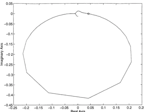
2-7 Locus of Plant Poles as Dynamic Pressure Varies . ... 49

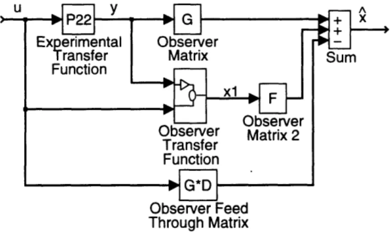
3-1 Block Diagram of Observer Implementation . ... 53

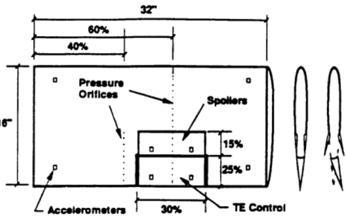
4-1 The Benchmark Active Controls Technology (BACT) Model .... . 62

4-2 Top View Sketch of the PAPA Assembly (Fairing Not Shown) . . .. 63

4-3 Robustness Analysis Diagram with Weighting Matrix . ... 70

4-4 Example Plot of the Maximum Eigenvalue of the Robustness Analysis Transfer Function ... ... .. 72

4-5 Measure of the Accuracy of the Predicted Flutter Dynamic Pressure (q) 77 4-6 Analytical Flutter Boundary ... .... 77

4-7 Enlargement of Portion of the Analytical Flutter Boundary ... 78

4-8 Measure of the Accuracy of the Predicted Flutter dynamic Pressure (q) for Systems Augmented with Proportionality Matrices at Incorrect Nominal Values ... ... 81

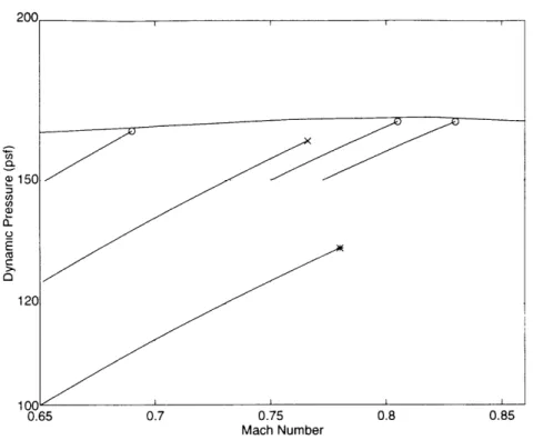
4-9 BACT Active Controls Testing Open Loop Flutter Boundary .... . 83

4-10 Full Order Analysis D(s)B for Low Mach Number Transfer Functions 86 4-11 Reduced Order Analysis 1(s)B for Low Mach Number Transfer Functions 87 4-12 BACT Model 1 Flutter Boundaries . ... . . . . . 88

4-13 BACT Model 3 Flutter Boundary for Perturbations in Mach Number and Dynamic Pressure ... ... . . 90

4-14 Model 3 Flutter Boundary Including Both Robustness Analyses . . . 92

B-i Perturbed Transfer Functions: 25% Perturbation in Dynamic Pressure. 110 B-2 Perturbed Transfer Functions: 50% Perturbation in Dynamic Pressure. 111 B-3 Perturbed Transfer Functions: 75% Perturbation in Dynamic Pressure. 112 B-4 Perturbed Transfer Functions: 15.4% Perturbation in Mach Number. 113 B-5 Perturbed Transfer Functions: 26.2% Perturbation in Mach Number. 114 B-6 Perturbed Transfer Functions: 38.5% Perturbation in Mach Number. 115 C-1 Block Diagram of Perturbed Parametric Model ... 121

C-2 Multi-Variable Integrator for State Space Systems . ... 124

C-3 BACT Model Nominal Actuator Block . ... 124

C-4 BACT Model Nominal Aerodynamic Block . ... . 125

C-5 BACT Model Nominal Plant Aerodynamic Lag Terms ... . 127

C-6 BACT Model Nominal and Perturbed Plant Structural Terms . . . . 128

C-7 BACT Model Perturbed Plant Aerodynamic Lag Terms for Variations in the Scaling Factor () ... 131

C-8 BACT Model Perturbed Plant Aerodynamic Lag Terms for Variations in Dynamic Pressure . ... ... 131

List of Tables

2.1 Percent Errors in Reconstructed System for Dynamic Pressure

Pertur-bations. ... ... ... 35

2.2 Percent Errors in Reconstructed System for Mach Number Perturbations. 35 2.3 Eigenvalues of Perturbed BACT Models - Nominal q = 75psf ... . 46

2.4 Error in Predicted Eigenvalues of Perturbed BACT Models. ... 47

4.1 Summary of Robustness Analysis of Analytical Data . ... 76

4.2 Predicted Analytical Transfer Functions Flutter Points Resulting from the Use of Proportionality Matrices at Incorrect Nominal Values . . . 80

4.3 Nominal Conditions of Experimental Transfer Functions for Robust-ness Analysis ... .. ... .. 84

4.4 Summary of Results of Model 3 Analysis for Perturbation in Mach number and Dynamic Pressure ... ... 89

4.5 Summary of Results of Model 3 Analysis for Perturbation in Dynamic Pressure Only ... ... .. 91

B.1 Summary of BACT model States, Inputs, and Outputs ... 103

B.2 Summary of Flight Conditions of BACT models . ... . 104

B.3 SSQ: Mach Number = 0.75; Dynamic Pressure = 125psf ... 105

B.4 Notation and Structure of ISAC SSQ . ... 106

B.5 Summary of Proportionality Matrix Nominal Conditions for the BACT models ... ... ... 107

B.6 Proportionality Matrix . . . ... ... ... 108

B.8 Parameterized Method Example 31 Augmentation Matrix ... 117 B.9 State Space Method Example ac Augmentation Matrix ... 118 B.10 State Space Method Example Pi Augmentation Matrix ... 119

C.1 Description of Individual Blocks in Actuator Dynamic Subsystem . 125 C.2 Description of Individual Blocks in Aerodynamic States Subsystem . 126 C.3 Description of Individual Blocks in Plant Aerodynamic Lag Term

Sub-system ... .. ... ... . 127 C.4 Description of Individual Blocks in Plant Structural Term Subsystem 128 C.5 Description of Individual Blocks in Plant Structural V Perturbation

Subsystem ... ... . . . . .... ... . 129

C.6 Description of Individual Blocks in Plant Aerodynamic Lag, - Pertur-bation Subsystem ... ... .. . ... ... . 130 C.7 Description of Individual Blocks in Plant Aerodynamic Lags, Dynamic

Chapter 1

Introduction

1.1

Motivation

In a world of rapidly evolving aircraft technology, designers are becoming increasingly concerned with the robustness of systems to parametric uncertainties. The ability to predict a system's response to parametric or operating condition perturbations, as well as determine what variations will lead to an instability is an extremely useful tool when analyzing or designing complex aeronautical systems. However, the techniques necessary for determining the destabilizing perturbations were not available until the advent of modern robustness analysis. Algorithms based on structured singular value analysis began to evolve in the 1980's. Since then, the methods for calculating structured singular values, specifically purely real structured singular values have continually been improved to achieve a tighter bound on the solution while being less computationally intensive. New developments have also been made which allow a robustness analysis to be undertaken on experimentally obtained frequency dependent plant transfer functions. This thesis shows the application of such techniques on a specific concern facing aircraft designers, the instability of flutter.

Flutter can be defined as a self-excited, unstable oscillation resulting from the combination of elastic, inertial, and aerodynamic forces on a mass which, in this study, is a wing. As aircraft designs tend toward higher speeds and more flexible structures, the instability of flutter becomes more important. Also, as aircraft designs become

more complicated, the standard methods of modeling systems and predicting flutter may not be adequate [4]. The application of new robustness analysis techniques to classical flutter prediction provides one method of modernizing an old problem and analysis. Robustness analysis can not only be used to predict the flutter boundaries of analytical systems, but can be applied to experimental frequency domain transfer functions in order to determine the stability boundaries of complex physical systems. In flutter studies, the parameters of most concern are the varying flight condi-tions under which the system operates. For systems operating near the edge of their performance boundaries, the effects of perturbations in flight conditions such as dy-namic pressure and Mach number on the system's stability are of utmost concern and an accurate prediction of this performance boundary can be crucial. One spe-cific performance boundary, a system's flutter boundary, is often characterized by the combination of Mach numbers and dynamic pressures above which flutter will occur. This bound is typically obtained from an aerodynamic study and is confirmed exper-imentally though extensive wind tunnel testing. Robustness analysis offers another method for predicting this flutter boundary. The object is to characterize the effects of perturbations in Mach number and dynamic pressure on the system being studied. The robustness analysis then utilizes these characterizations, along with experimen-tally measured frequency domain plant transfer functions, to predict destabilizing perturbations in Mach number and dynamic pressure. The remainder of this the-sis will detail the steps necessary to perform such an analythe-sis and show the results when applied to the NASA Langley Research Center's Benchmark Active Controls Technology (BACT) model [8].

The techniques involved in performing a robustness analysis are as follows:

1. Defining the real parametric perturbations of concern in the analysis. (Section 1.1)

2. Characterizing the effects of the parametric perturbations on the elements of the analytical state space model of the system being studied.

(Sections 2.2.1 and 2.3.1)

3. Using the characterizations of step 2 to create a set of augmentation matri-ces which will be used to transform frequency domain input/output trans-fer functions into a transtrans-fer function which can be used for the robustness analysis.

(Sections 2.1.2, 2.2.2 and 2.3.2)

4. Transforming the experimental frequency domain data into a form com-patible with the augmentation matrices of step 3.

(Sections 2.1.3, 3.1 and 3.2)

5. Combining the results of step 3 and step 4 to obtain the final transfer function for the robustness analysis.

(Sections 2.1.3 and 3.2.3)

6. Performing the final analysis on the transfer function from step 5.

(Sections 2.1.4 and 4.3)

The reader is encouraged to refer back to this procedure while reading the detailed derivation of each step.

_ ^^ _

1.2

Outline

Step one, the definition of the upcoming robustness analysis, was stated earlier as the prediction of flutter boundaries in Mach number and dynamic pressure space. The procedures outlined above will be explained and tested through examples related to the effects of perturbations in Mach number and dynamic pressure on the Langley BACT model. Each of the following chapters will address a set of the robustness analysis steps, culminating with the results of the analysis applied to the BACT.

Chapter 2 describes the basic formulation of the robustness analysis problem for the study of flutter. A brief description of the basis of the analysis, taken from a previous study by Blaise G. Morton and Robert M. McAfoos, will be given [5, 6].

The second step of the analysis requires an accurate characterization of the effects of perturbations on the plant of interest. Chapter 2 will describe methodologies for characterizing these effects for two types of systems. First, methods for plants which are modeled analytically in state space form with no further insight into the internal dynamics of the system will be outlined. Second, plants for which a description of the internal dynamics is known will be detailed. Chapter 2 will describe not only how to characterize the effects of perturbations on the two types of systems, but show how to generate the augmentation matrices from step 3 above.

Chapter 3 utilizes the characterizations obtained from Chapter 2 to achieve the final robustness analysis transfer function. The methodologies for transforming ex-perimental frequency domain transfer functions into a form which is compatible with the augmentation matrices defined in Chapter 2 will be shown. Depending on the dimensions of the original plant, different methods are available to accomplish the transformation. First, the standard setup for systems with an equal number of states, inputs, and outputs will be shown. For more complicated systems with an unequal number of states, inputs, and outputs, an observer based method for transforming the system will be described. The observer based method implements a reduced order observer and a system identification process which together manipulate experimental frequency domain transfer functions into a format compatible with the

tion matrices. The resulting function and the augmentation matrices will, finally, be combined into the robustness analysis transfer function.

Chapter 4 outlines the results of the robustness analysis performed on the Langley BACT model. A description of the BACT model along with the experimental methods currently used by Langley to predict its flutter boundary will be discussed. The results of the analysis on both analytical and experimental frequency domain BACT transfer functions will be shown, and a comparison will be drawn between the flutter boundary obtained by Langley via their methods and the boundary derived by the robustness analysis. These results will be used to show the efficiency and limitations of the robustness analysis applied to flutter studies.

Chapter 5 will summarize the results of the study and present conclusions on the usefulness of robustness analysis for predicting flutter boundaries. Although this chapter completes the work for this thesis, it also suggests the future studies which should be conducted. These studies will continue to refine and utilize the robustness analysis for predicting flutter boundaries.

Chapter 2

Formulating a Robustness

Analysis Problem

The procedure for transforming experimental data into a system suitable for a ro-bustness analysis was adapted from a study performed by Blaise G. Morton and Robert M. McAfoos which applied a robustness analysis to a state space realization of the space shuttle in order to determine the system's stability under varying flight conditions. An overview of their procedure and its applicability to the analysis of ex-perimentally derived frequency domain transfer functions will be outlined in Section 2.1. The remainder of Chapter 2 will detail the method for achieving the second and third steps of the robustness analysis. In these steps, an examination of the effects of perturbations on the original analytical system is undertaken and a method for creating augmentation matrices which will model the effects of further perturbations is derived. Section 2.2 generalizes this step for systems with an analytical model already in state space form. Section 2.3 describes how systems not yet in state space form, but with known physical parameter such as mass and damping, can be formed into a robustness analysis problem. A system in this form will be referred to as a parameterized model in the remainder of the analysis. In each section, the description of the methodology will be followed by an example performed on the Langley BACT model.

2.1

Standard Problem Statement

The methods described in the Morton and McAfoos study will be used to complete the steps of the robustness analysis detailed in Chapter 1. An overview of these steps for a general system will first be presented. The specific modifications and applications of the methodologies for systems in state space and parameterized will be given in Sections 2.2 and 2.3, respectively.

2.1.1

Characterizing Perturbation Effects

The standard form of the state space equations of motion is shown in equation 2.1. A B

The matrix will be referred to throughout this thesis as the state space C D

quadruple or simply the SSQ.

= (2.1)

The second step in the robustness analysis study characterizes the effects of per-turbations on the system of interest. For systems with an analytical model in state space form, it is assumed that the connection between changes in each parameter and changes in the elements of the state space quadruple can be approximated by a linear function of the form given in equation 2.2,

A B n A, Bz

E6 (2.2)

C D z=1 Ci Di

where

is a matrix representing the changes in the SSQ due to -the sum of the effects of

Ai Bi

therefore C, Di represents a matrix of proportionality constants between the ith perturbations and the change in each element of the SSQ. The matrix

Az B, Ci D

will be referred to as the proportionality matrix of the ith parameter or simply the pro-portionality matrix. There are exactly n propro-portionality matrices, each corresponding to one particular perturbation parameter.

The system under any known perturbation can then be represented as the sum of equation 2.1 and 2.2 as shown by equation 2.3.

= + ei (2.3)

y CD z=1 Ci Di Lu

2.1.2

Creating Augmentation Matrices

The third step of the analysis requires a set of augmentation matrices be developed which can transform the original system into the form necessary for robustness anal-ysis. In the case of analytical systems described in a state space format, each of the

n proportionality matrices is decomposed into the augmentations matrices shown in

equation 2.4.

Ai

2

Bi

=

[

e:

]

(2.4)

Ci Di Ce2i

A procedure for accomplishing this will be shown in Section 2.2. Once augmentation matrices for each perturbation are created, they are combined by methods also shown in Section 2.2 to create the set of matrices ultimately used for augmentation, denoted as a,, a2, 01,7

2-Alternatively, if the analytical system is described by a set of physical parameters, a more explicit study of the effects of perturbations on the dynamics of the system is possible. In order to characterize the effects of perturbations on systems in this form,

an analysis of the differential equations of motion is done. The nominal values of the perturbation parameters can be found explicitly in the equations of motion and represent the locations where perturbations enter the system. The perturbations, which represent 6, in equation 2.3, can be entered directly into the equations of motion and a study of their effects can be done.

To calculate the augmentation matrices for parameterized models, the equations of motion including the perturbations parameters are used to create a block diagram model of the system. The equations of motion and block diagrams are rearranged so that the perturbation parameters act as the inputs and outputs of the system. The state space characterization of the new model, including the effect of parametric variation, directly yields the ac and 01 augmentation matrices described previously. This process will be described more thoroughly in Section 2.3.

2.1.3

Obtaining the Robustness Analysis Transfer Function

Irrespective of the format of the original system, the calculation of augmentation matrices allows the system to be transformed from the original plant transfer function from the known input (u) to the measured output (y) of Figure 2-la to the form of Figure 2-1b which is suitable for performing a robustness analysis.

-A

u G (s) - Y

nom

I I

(a) Original Plant Transfer (b)

Function

Figure 2-1: Experimental Transfer Functior

Upert Ypert

-_I - _L

I(s)-M(s) Robustness Analysis Form

n Block Diagrams

plant input to output transfer function of the form shown in equation 2.5.

Gnom(s) = C(s)B + D (2.5)

where

S1(s) = [sI - A]

-H(s) is an optional controller transfer function. In the following robustness analysis,

only open loop systems will be considered and, therefore, the effects of the controller transfer function will not be addressed. The A-block in Figure 2-1b is a diagonal matrix whose elements are real values representing the parameters in the perturbation study. The function P(s) is the new input to output transfer function matrix obtained when Gnom(s) is properly combined with the augmentation matrices. P(s) consists of the four independent transfer functions shown in equation 2.6.

_[P(s) P12(s)" Ypert = P11(S)Upert + P1 2 (S)U

P(s) = P2 1(s) P22(s) Y - P21(S)Upert + P22(s)u

(2.6)

The P 1l(s) and P21(s) components of the P(s) matrix show the effects of the input perturbations upert on the output perturbations Ypert and the.original output y, respectively. The P12(s) component relates the original plant input u to the output

perturbations Ypert. The final transfer function P22(s) is the original input to output transfer function Gnom(s) as shown in equation 2.7.

P2 2 () = Gnom(s) (2.7)

The last function in the robustness analysis diagram is M(s) which is the total transfer function from the input perturbation upert to the output perturbation Ypert. For systems with an implemented controller transfer function H(s) in the feedback path of the robustness analysis diagram, M(s) is calculated by equation 2.8.

If the feedback loop from the nominal output y to the input u is open, M(s) reduces to the equality of equation 2.9.

M(s) = Pu (s) (2.9)

In the study by Morton and McAfoos, the P matrix is represented by the aug-mented plant in state space form shown in equation 2.10. The system represents a set of three linear dependent matrix equations.

A " ax B

Ypert Upert (2.10)

y U

C 2 D

The frequency domain augmented system, P(s), can be derived by taking the Laplace transform of the first rows of equation 2.10 corresponding to the states and substituting the result into the remaining two matrix equations for the perturbed and nominal outputs. The Laplace transform is shown in equation 2.11 and the final augmented system after the substitution is given in equation 2.12.

X = (P(8) [al upert + Bu] (2.11)

01 D(s)aj O:(D(s)B + 02

Ypert

]

..

(2.12)

C(s)al + 2 CD(s)B + D

Each component of the P(s) matrix can be individually calculated. The matrix element located in the lower right corner of the P(s) matrix of equation 2.12 con-tains the original transfer function Gnom(s) as stated previously in equation 2.7. The other matrix elements of P(s) contain portions of the original transfer function which are combined with the augmentation matrices qualitatively described previously. A formal method of calculating the augmentation matrices will be given in Section 2.2.

Methods for incorporating the experimentally obtained transfer functions into equa-tion 2.12 will be described in Chapter 3.

Once the P(s) matrix is calculated, an estimate of the perturbed transfer func-tion when the values in the A-block are known can be determined directly from an examination of the closed loop robustness analysis diagram and a combination of the transfer functions in equation 2.6. The result, denoted Gpert(s), is shown in equation 2.13. If some insight into the effects of perturbations on the systems is available, and calculations of Gpert(s) will show if the augmented system responds to perturbations in the expected manner.

Gpert(S) = P21 (s)A [I - P1 (s)A]- 1 P12(s) + P22(s) (2.13)

The study by Morton and McAfoos showed that the setup of Figure 2-1b does, in fact, exactly model the system in equation 2.3. In their study, the real structured singular value analysis results for a baseline plant and flight controller predicted an in-stability at low frequencies. Subsequent test confirmed that a set of real perturbations did exist which caused the low frequency instability to occur [6].

2.1.4

Solving the Robustness Analysis

After the perturbation characterization has been completed and and the robustness analysis transfer function has been formed, the final analysis can be performed. The result of the analysis is a quantification of the smallest destabilizing perturbation of the parameters existing in the A-block. A solution exists only at frequencies where a real parametric variation will cause the system to go unstable. This solution, shown analytically in equation 2.14, is defined as the maximum singular value of the A-block with the minimum norm which causes the determinant of [I - M(s)A] to be equal to zero.

1

- = min{((A)I det(I - M(s)A) = 0} (2.14)

Algorithms afor solving

Algorithms for solving a robustness analysis problem when the number of

eters is large or the parameters appear as blocks of repeated real values are com-putationally intensive and produce upper and lower bounds on the solution. In the case of flutter studies, however, computations can be simplified by introducing a re-lation between the Mach number and dynamic pressure to the total pressure (H) of the system, reducing the A-block to an identity matrix multiplied by a real scalar 6. A method of obtaining a A-block in this form from one which originally contains multiple parameters will be explored further in Chapter 4 during the application of the robustness analysis to experimental flutter. The solution to the simplified prob-lem can be found by looking only at the eigenvalues of the M(s) matrix shown in Figure 2-lb. The minimum destabilizing perturbation is given by the inverse of the maximum eigenvalue, as shown in equation 2.15.

1

6 - (2.15)

A(M(jw*))

A derivation of equation 2.15 is presented in Appendix A.

2.2

State Space Model Based Methods

The first type of system to be considered is one which exists analytically in state space model form. No significant knowledge of the physical dynamics of the system is assumed and, therefore, the characterization of the effects of perturbations on the physical system can be done quantitatively only on the separate elements of the state space quadruple. Very little physical insight can be drawn as to the effect of perturbations on the individual physical parameters of the system. However, a robustness analysis of the state space quadruple will still yield the perturbation which destabilizes the overall system.

2.2.1

Characterizing Perturbation Effects

The first step for constructing any realistic robustness analysis problem is accurately defining a complete set of parameters to appear in the A-block. Although limiting

the number of parameters in the study simplifies the subsequent computations, care must be taken not to exclude parameters which may be vital in accurately describing the process being studied. Once this set of parameters is established, their effects on the state space quadruple must be quantified in order to derive the proportionality matrices of Section 2.1.

Describing the changes in the state space quadruple due to parametric variation requires a reasonable bank of analytical models. One of the models must be defined as the nominal model and be created with each perturbation parameter set at their respective nominal values. The state space quadruple associated with the nominal value of all the parameters of interest is designated as:

C D

- nom

In order to characterize the effect of each parameter individually, several additional models must be created by varying one parameter at a time while holding all other parameters at their nominal values. For the ith parameter, this leads to a set of state space quadruples, each created at a particular perturbation value. These can each be represented as:

C I pert,z

The proportionality matrix of the ith parameter is calculated by finding a linear relationship between the nominal and perturbed state space quadruple which satisfies equation 2.16.

= _{+ i Di 6i (2.16)}

Spert,i C D nom i

To determine the elements of the proportionality matrix, consider the linear equa-tion for each element separately. If the element in the jth row and Ith column is desig-nated as el(,3 )1, the independent linear relation is represented by equation 2.17. The

solution of this equation for el(2,)2 is trivial and can be recognized as the slope (m) of the line, y = b+mx, where the y-axis represents the value of the particular perturbed matrix element, el(3,l)pert, , and the x-axis is the perturbation of the parameter under

consideration, 6,.

el(3,1)pert,z = e1(,).o... + el(3,1)1, (2.17)

If the perturbation parameter has a linear effect on changes in the state space quadruple, each element of the proportionality matrix, el(J,)pert, , will be independent

of the amplitude of 6,. If, instead, some variation occurs for different amplitudes of 6, then a least squares fit is used to obtain el(,Il)2. The slope of the least squares

fit represents the value of the specific element of the proportionality matrix, el(3,l) . To complete the derivation of the proportionality matrix, this process is repeated for every element of the SSQ and for perturbations for each parameter of interest, separately. Section 2.2.4 presents a numerical example of this procedure.

2.2.2

Creating Augmentation Matrices

Once proportionality matrices have been formed, the next step is to create the aug-mentation matrices necessary to correctly transform the experimental plant into the robustness analysis form. As shown previously by equation 2.4, a pair of augmenta-tion matrices must be formed from each proporaugmenta-tionality matrix. The augmentaaugmenta-tion matrices are not unique and their values depend on the method used for decomposing the proportionality matrix. Although there are several valid methods of decomposing the proportionality matrices, the desired method will result in the smallest possible dimensions of the columns and rows of a, and 3, respectively. The reason for reduc-ing the dimensions of the augmentation matrices can be traced back to the derivation of the augmented plant in equation 2.12. If the number of columns and rows in ca and 0, is small, the resulting dimensions of the augmented plant is small, as well. Reducing the order of the augmented plant, in turn, simplifies the solution of the robustness analysis. One possible method of generating these matrices which allows the dimensions of a, and 0, to be reduced, and the one used subsequently in this

analysis, is to perform a singular value decomposition (SVD) on the proportionality matrix. The standard form of an SVD is given by equation 2.18.

, Bi [U U2 , Si i (2.18)

The matrices U, and VIH are the orthonormal left and right singular vectors, respec-tively, and Si is a diagonal matrix of singular values which may or may not be full rank. To calculate the augmentation matrices, retain all of the non-zero singular values of S, and their corresponding columns and rows of U and ViH . Combining the relations of equations 2.4 and 2.18 results in the final equation for creating the

augmentation matrices shown in equation 2.19.

UljS 2VH = aii (2.19)

The simplest solution to equation 2.19 is shown in equation 2.20

3i = SV H (2.20)

The process is repeated for the proportionality matrix resulting from every parametric perturbation.The resulting ai and O3 are partitioned into the two matrices shown in equation 2.4 and the final augmenting matrices are constructed by stacking the matrices of each perturbation in the manner shown in equation 2.21.

P11 012 S2 212 _{22 (2.21)} (Y2 2122

_I

The dimension of the augmentation matrices can be gleaned by an inspection of their derivation. One dimension of each of the augmentation matrices will be equal

to that of one of the various state space matrices; a, has the same number of rows as does the A matrix, whereas 1 has the same number of columns as the A matrix. The other dimension is determined during the singular value decomposition and is equal to the number of singular values retained during the calculation of equation 2.20. The maximum size of this dimension is constrained by the rank of the proportionality matrix being decomposed. The minimum dimension, however, can be specified during the calculation of the augmentation matrices in equation 2.20.

The number of non-zero singular values retained in the calculation, and their relative magnitudes, is a function of the rank of the proportionality matrix. If a perturbation affects several elements of the SSQ, the proportionality matrix may be full rank, or nearly so, and few or none of the singular values will be zero. Typically, however, some elements of the SSQ are more influenced by perturbations than others and the result is a range of singular values in equation 2.18 spanning several orders of magnitude. Low order singular values can be treated as consequences of computa-tional errors or as results of insignificant perturbation effects and concluded to offer little to enhancing the accuracy of the augmented model.

Therefore, to decrease the second dimension of the augmentation matrix and thereby speed subsequent computations, some of the smaller singular values can be truncated along with those that are truly zero. The key is not to truncate an exces-sive number of singular values, as the accuracy of the analysis will be sacrificed for speed. A guide to determining if and which singular value can be excluded can be ascertained by reversing the augmentation matrix computations and attempting to reconstruct the original perturbed plant of equation 2.16.

First, several augmentation matrices are created for one perturbed plant by re-taining different numbers of singular values in the calculation of equation 2.20. The steps for creating a and 3 are then reversed by applying equation 2.4 to recreate an approximate proportionality matrix.

- approx

Next, equation 2.16 is applied, using the approximate proportionality matrix, to obtain a perturbed state space quadruple.

I

To compare the two systems, a frequency response of the actual perturbed plant used in equation 2.16 and the approximated perturbed plant derived above can be obtained and the error between the resulting transfer functions examined. An example of this procedure will be given in Section 2.2.4.

2.2.3

Example of State Space Models

A state space representation of the NASA Langley Research Center's BACT model is used to illustrate the methods shown in this section. A basic description of the dimensions and states of the model is presented in the following paragraph as well as in Appendix B. A more detailed account of the BACT program, physical model and the algorithms used to derive the state space model is given in Chapter 4.

The BACT model is a NACA 0012 airfoil model used for flutter studies and control law analysis. The initial analytical state space model includes two elastic modes, plunge and pitch, and one control mode due to a second order model of a trailing edge actuator. Each mode is represented by two generalized states. In addition, the aerodynamic forces are modeled by three aerodynamic lags each contributing two states to the model. Finally, the full order system contains two states for modeling the gust spectra dynamic characteristics resulting from white noise passed through a gust filter. The gusts states are removed prior to the robustness analysis, leaving a final analytical model with twelve states. The input to the model can be a command to the actuator or gust input. Again, the influence of the gust input is removed, leaving one input into the BACT model. The outputs of the analytical model relevant in the robustness analysis are the measurements of the four accelerometers located about the perimeter of the model. The final dimensions of the reduced order state space

model contain twelve states, one input, and four outputs.

2.2.4

Application to Example Case

The characterization of the effects of perturbations on the Langley BACT model will now be performed. As stated previously, the dynamic process of main concern is flutter, therefore, the effects of perturbations in dynamic pressure and Mach number, the parameters which describe typical flutter boundaries, will be studied. The first step is to create the proportionality matrices; one for dynamic pressure perturbations and one for Mach number perturbations. To do this, 56 analytical state space mod-els were created at combinations of different nominal Mach numbers and dynamic pressures. The Mach numbers included: 0.3, 0.5, 0.65, 0.75, 0.77, 0.82, and 0.9. The dynamic pressures ranged from 75psf to 250psf at intervals of 25psf. An example of a state space quadruples of the BACT model can be found in Appendix B. When generating the elements of the proportionality matrices, plots of the least square fits described by equation 2.17 were generated. The results showed that dynamic pressure has a linear effect on most changes in the SSQ whereas Mach number has a highly non-linear effect.

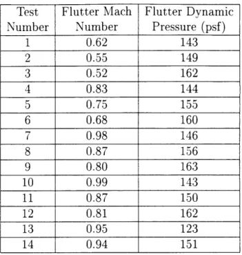
To demonstrate this, first a plot of the A(3, 4) state space element, representing the influence of the pitch rate state on the derivative of the plunge rate state, ver-sus perturbed values in dynamic pressure is presented in Figure 2-2. The nominal dynamic pressure was set at 150psf and the nominal Mach number was held at 0.5. The nominal plant is represented by the point at the origin of the plot in Figure 2-2. Plants at seven perturbed values of dynamic pressure with a nominal Mach number of 0.5 were used in the linear fit. The plot indicates that changes in dynamic pressure do have a linear effect on changes in the state space elements as each point, representing el(3,4)q for a plant at a different perturbed value of dynamic pressure, coincide on a line of constant slope. The slope of the line through the points is the value of the proportionality matrix for the element Ai(3, 4). Note that perturbations as large as 67% of the nominal dynamic pressure remain along a line of constant slope. There-fore, the proportionality matrix provides an accurate measure of how changes in the

E

-5

-10

-80 -60 -40 -20 0 20 40 60 80 100 Perturbation in Dynamic Pressure (Nominal of 150psf)

Figure 2-2: Linear Relation Between Perturbations in Dynamic Pressure and in the SSQ

state space quadruple occur in response to perturbations implying that a robustness analysis performed using dynamic pressure should be accurate.

To demonstrate the changes in elements of the state space quadruple when the perturbation parameter has a non-linear effect, the results of perturbations in Mach number on changes in the A(3, 4) element of the BACT model are shown in Figure 2-3. Plants derived at six perturbed Mach numbers around a nominal value of 0.75 independently produced the values of el(3,4)M shown by the points on Figure 2-3.

The slope of the line representing the least squares fit through the points becomes the approximate value of the Ai(3, 4) element of the proportionality matrix. Here, perturbations of more than 10% from the nominal Mach number cause a non-linear change in the element. To reduce the error induced by this nonlinearity, only narrow

ranges of Mach numbers can be considered when performing the linear fit.

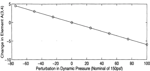
The Mach numbers were, therefore, broken into three ranges: low, medium, and high. The low range consisted of Mach numbers between 0.3 and 0.65. The medium range ran between 0.65 and 0.77 and, finally, the high range included Mach numbers between 0.77 and 0.9. Proportionality matrices were created for each of these ranges. The results of the linear fit, again for the A(3, 4) element, are shown in Figures 2-4a to 2-4c. Within each range, the maximum errors of the calculated A(3, 4) point from the

10 .c -5 1 -10 < o -15

-

Perturbation in Mach Number (Nominal of 0.75)

Figure 2-3: Non-linear Relation Between Perturbations in Mach Number and in the SSQ

linear fit are 11.6%, 2.2%, and 27.6%, low to high range, respectively. Compared to the maximum error of 84.3% when the whole range of Mach numbers was analyzed, the method of segmenting the ranges of non-linear parameters shows a large improvement. A listing of the nominal conditions of all the proportionality matrices used in the study, and an example matrix, can be found in Appendix B.

After the proportionality matrices have been derived, the next, step is calculating the augmentation matrices. In order to speed subsequent calculations, the order of the augmentation matrices was systematically reduced to achieve the smallest possi-ble dimensions while maintaining accuracy in predicting the effects of perturbations on the system. The accuracy of the reduced order augmentation matrices can be tested by the method described in Section 2.2.2. In the case of the BACT model, full order augmentation matrices contained thirteen perturbations due to dynamic pressure and thirteen due to Mach number. Reduced order augmentation matrices were obtained by truncating the number of singular values retained during the com-putation of the augmentation matrices in equation 2.20. The reductions were done for each perturbation parameter separately and the resulting augmentation matrices were used to reconstruct the perturbed system. Each transfer functions from the input to the four accelerometer outputs of the original and reconstructed perturbed system

(a) -- Mach numbers Range = 0.3 - 0.65 2 0 8 6 4 2-0 0.05 2.5 2 ,,i 1.5 U) a) 0.5 0.1 0.15 0.2 0.25 Perturbation in Mach Number (Nominal of 0.3)

(b) -- Mach numbers Range = 0.65 - 0.77

0.04 0.06 0.08 Perturbation in Mach Number (Nominal of 0.65)

(c) -- Mach numbers Range = 0.77 - 0.90

0.3 0.35

1 0.12

0.04 0.06 0.08 0.1

Perturbation in Mach Number (Nominal of 0.77)

Figure 2-4: Linear Fits to Perturbations in the SSQ due to Reduced Number

Ranges of Mach

can be compared. The error resulting between the two transfer functions provides a measure of the accuracy of the reduced order augmentation matrices in predicting the effects of perturbations on the plant SSQ. Placing a bound on the maximum al-lowable error constrains the number of singular values which can be truncated during the calculations.

The tabulated results of the average error of the reconstructed perturbed system are shown in Tables 2.1 and 2.2. The errors were calculated by taking the difference of the actual and reconstructed perturbed transfer functions and normalizing by the nominal transfer function. The magnitude and phase plots of the transfer functions used to obtain the tabulated data are located in Appendix B. The errors in the tables show that some of the singular values associated with each perturbation can be truncated without any loss of accuracy in the system reconstruction. However, after a point, the remaining singular values are critical to assure accurate results from the robustness analysis.

Table 2.1 shows that the order of the augmentation matrices associated with dy-namic pressure can be greatly reduced without significant loss of accuracy. Retaining only two of the thirteen original singular values when creating the augmentation ma-trices yields the same accuracy as when recreating the perturbed system using a full order augmentation. The dimensions due to the Mach number perturbations can not be reduced as extensively before losing accuracy. In this case, Table 2.2 shows that re-taining eight of the original thirteen singular values allows for an accurate description of the perturbed system. Removing two additional singular values, leaving six, yields a slightly less accurate result. Decreasing the number of singular values any further yields an augmented system which does not emulate the actual perturbed system.

The final dimension of the A-block was established at ten: two perturbations corresponding to dynamic pressure and eight to Mach number. The dimensions were chosen as the lowest size which still represented the perturbed system with the same accuracy as the full order augmentation. The resulting A-block has the form shown

Table 2.1: Errors in Reconstructed System for Dynamic Pressure Perturbations. Nominal Dynamic Pressure = 100psf. Nominal Mach Number = 0.75.

Values Represent Percent Errors

% 1 # a iOutput 1/Input Output 2/Inputj Output 3/Input Output 4/Input

Mag. Phase Mag. Phase Mag. Phase Mag. Phase

13 0.004 0.001 0.001 0.001 0.004 0.001 0.001 0.001 2 0.004 0.001 0.001 0.001 0.004 0.001 0.001 0.001 25 1 14.9 1.88 14.2 3.08 14.6 1.88 14.2 3.08 13 0.005 0.001 0.005 0.001 0.005 0.001 0.005 0.001 2 0.005 0.001 0.005 0.001 0.005 0.001 0.005 0.001 50 1 31.0 3.51 27.3 4.07 30.9 3.48 27.3 4.08 13 0.015 0.001 0.002 0.001 0.014 0.001 0.002 0.001 2 0.015 0.001 0.002 0.001 0.014 0.001 0.002 0.001 75 1 50.2 4.83 39.4 4.46 49.3 4.80 39.4 4.46

Table 2.2: Errors in Reconstructed System for Mach Number Perturbations. Nominal Mach Number = 0.65. Nominal Dynamic Pressure = 125psf. Values Represent Percent Errors.

Yc 'm # a Output 1/InputllOutput 2/InputllOutput 3/Input Output 4/Input

Mag. Phase Mag. Phase Mag. Phase Mag. Phase

13 0.321 0.045 0.067 0.247 0.317 0.046 0.066 0.247 8 0.321 0.045 0.067 0.247 0.317 0.046 0.066 0.247 6 0.246 0.042 0.79 0.178 0.243 0.043 0.079 0.178 15.4 5 7.62 0.119 7.40 1.02 7.51 0.103 7.40 1.02 13 4.01 0.534 0.880 2.83 3.96 0.544 0.879 2.83 8 4.01 0.534 0.880 2.83 3.96 0.544 0.879 2.83 6 4.16 0.524 0.823 2.97 4.11 0.536 0.822 2.97 26.2 5 17.4 0.482 11.8 5..10 17.0 0.449 11.8 5.10 13 20.9 3.00 4.50 13.7 20.6 3.03 4.50 13.7 8 20.9 3.00 4.50 13.7 20.6 3.03 4.50 13.7 6 21.2 2.95 4.35 13.9 20.9 3.00 4.35 13.9 38.5 5 40.4 2.65 16.7 17.2 39.7 2.96 16.7 17.2

in equation 2.22.

Iq 6q

₀

0 I6M (2.22)

The variable 6 represents a real perturbation of the parameter indicated by the sub-script. Each identity matrix has a dimension equal to the number of singular values retained in the augmentation matrix calculations for the parameter indicated by the subscript. The final augmentation matrices have the dimensions shown in

equa-tion 2.23.

a₁ = 12x10

a₂ = 4x10 1 = 10x12

32 = 10xi (2.23)

2.3

Parameterized Model Based Methods

An alternate method for characterizing the effects of parametric perturbations can

be conducted on systems which have known physical parameters. In this case, the parameters such as the system mass, stiffness, damping, and physical dimensions, are known and are used to assemble an analytical expression for the dynamics of interest in the robustness analysis. From the location and relation of the perturbing parameters to the other physical constants of the system, a more explicit understanding of the effects of parameter variation can be gleaned.

2.3.1 Characterizing Perturbation Effects

In order to begin characterizing the perturbation effects, the location of all the per-turbation parameters in the dynamic expression must be noted. For systems where several different perturbations parameters are being considered, each must occur lin-early and independently throughout the equation, otherwise steps must be taken to

place the equations in this form. The first step for creating the relation characterizing the effects of multiple perturbations is to ensure that every perturbation is decoupled. Methods for decoupling multiple perturbations depend on the structure of the orig-inal dynamics and, therefore, will be discussed later in Section 2.3.4 in conjunction with the BACT model example.

Once the perturbations are decoupled, the nominal parameters are replaced with an expression which takes into consideration the effects of perturbations on the sys-tem. Perturbations can be entered into the system by defining the perturbed param-eter as the sum of a nominal and varying value, as shown for a random variable X in equation 2.24.

X = Xnom -+ 6X (2.24)

If any of the perturbed values resulting after equation 2.24 is inserted into the ex-pression for the dynamics have an order greater that one, the equation must be linearized. As an example, if the variable X occurs as a squared term, the perturbed system would be linearized by the approximation of equation 2.25.

X2= (Xnom +6X) = X2om + 2Xnom6X + (6X)2

Xnom + 2Xnom6X (2.25)

Other methods of linearizing the perturbations are possible and must be employed per the specific structure of the plant under consideration.

2.3.2

Creating Augmentation Matrices

In order to derive the augmentation matrices, first the dynamic equation containing the parametric perturbations are transformed into a state space representation. The inputs and outputs of the state space system are exactly the perturbations entered into the dynamic expression through equation 2.24. In transfer function form, this represents the Pul(s) portion of the augmented P(s) matrix and is shown in equa-tion 2.26. As previously stated, if the robustness study is being conducted on an open

loop system, only the Pl I(s) component contributes to the overall robustness analysis

M(s) matrix. Thus, only ca and 31 need to be calculated.

ypert =- (P1((S)a1)Upert (2.26)

One method of creating the transfer function of equation 2.26 and, more impor-tantly, the matrices which comprise it, is to set up a block diagram description of the perturbed dynamic equation. The new block diagram has one input and one output corresponding to each location of a perturbation in the dynamic equation. An analy-sis of the diagram will produce a state space representation of the system in the form shown in equation 2.27.

S= AbdX + BbdUpert

Ypert CbdUpert (2.27)

P- analogy to the transfer function in equation 2.26, ca is equal to the Bbd matrix of equation 2.27, and /3 is equal to the Cbd matrix.

2.3.3

Example of Parameterized Models

As an example, the physical parameters of the BACT model used to derive the state space models described in Section 2.2.3 are represented in a dynamical expression for flutter studies. In addition to the physical mass, spring, damping, and dimensions of the BACT model, a description of the frequency dependent unsteady aerodynamic forces effecting the system is available. In order to incorporate the aerodynamic force data into a state space formulation of the dynamics, the generalized aerody-namic forces, denoted

Q,

sb sb2 (2.28)

Q = Ao + AV + A2 A2+ V (2.28)

The variable b is the model reference chord and V is the free stream velocity. Each

L, term is a constant denominator coefficient for the 11 aerodynamic lags. Finally, s

is the Laplace operator.

The aerodynamic coefficients, A2, are least square best fits to tabular aerodynamic force data at a specific Mach number and range of frequencies. The aerodynamic co-efficients are partitioned matrices with elements which independently effect the gen-eralized plant, actuator, and gust states. The partitioning is shown in equation 2.29.

A, AI A] (2.29)

The aerodynamic coefficients, A,, constant denominator coefficients, L,, and the remaining physical parameters of the system are combined into a dynamic expression for the BACT model states defined in Section 2.2.3. If the states are restricted to the generalized physical states (i), aerodynamic states (xa), and the actuator states, including positions (6), rates (6), and accelerations (6), the resulting dynamic equations governing flutter are shown in equation 2.30.

d2( b d(

- 4 d- = (Kg - qA + (D E - qA) - qA ax

6 b .d6 b 2 d 2

-qA 6 - q-Ai + (M - q() ) dt2A

dx A = A + A d V 3 (2.30)

dt j+2 dt j +2 _{dt b}

The dynamic pressure appears explicitly in the equation as q. The matrices K and D E are the generalized stiffness and damping terms, respectively. M 6 is a mass coupling matrix between the actuators and generalized states. The coefficient Aia is a matrix of ones and zeros, as defined in reference [1], relating the effects of the aerodynamic lags on the individual generalized states. The M matrix, shown in equation 2.31, is a mass matrix formed from the combination of the generalized mass matrix, Mg, and the aerodynamic coefficient, A2, as follows:

M = - q( )2A (2.31)

A M