HAL Id: hal-00526589
https://hal.archives-ouvertes.fr/hal-00526589
Submitted on 15 Oct 2010HAL is a multi-disciplinary open access archive for the deposit and dissemination of sci-entific research documents, whether they are
pub-L’archive ouverte pluridisciplinaire HAL, est destinée au dépôt et à la diffusion de documents scientifiques de niveau recherche, publiés ou non,
An X-FEM and Level Set computational approach for
image-based modeling. Application to homogenization.
Grégory Legrain, Patrice Cartraud, Irina Perreard, Nicolas Moës
To cite this version:
Grégory Legrain, Patrice Cartraud, Irina Perreard, Nicolas Moës. An X-FEM and Level Set compu-tational approach for image-based modeling. Application to homogenization.. International Journal for Numerical Methods in Engineering, Wiley, 2010, 86 (7), pp.915-934. �10.1002/nme.3085�. �hal-00526589�
GeM Institute
GeM Institute UMR CNRS 6183
´
Ecole Centrale de Nantes / Universit´
e de Nantes / CNRS,
1 Rue de la No¨
e, BP92101, 44321 Nantes, France.
An X-FEM and Level Set
computational approach for
image-based modeling.
Application to homogenization.
G. Legrain, P. Cartraud, I. Perreard, and
N. Mo¨es
Preprint submitted to:
International Journal for Numerical Methods in
En-gineering
An X-FEM and Level Set computational approach for
image-based modeling. Application to homogenization.
G. Legrain11, P. Cartraud1, I. Perreard2, and N. Mo¨es1
1
GeM Institute UMR CNRS 6183 - ´Ecole Centrale de Nantes / Universit´e de Nantes / CNRS, 1 Rue de la No¨e, BP92101, 44321 Nantes, France.
2
Dartmouth Medical School (USA) and Dartmouth Hitchcock Medical Ctr. (USA)
SUMMARY
The advances in material characterization by means of imaging techniques require powerful computational methods for numerical analysis. The present contribution focuses on highlighting the advantages of coupling the Extended Finite Elements Method (X-FEM) and the level sets method, applied to solve microstructures with complex geometries. The process of obtaining the level set data starting from a digital image of a material structure and its input into an extended finite element framework is presented. The coupled method is validated using reference examples and applied to obtain homogenized properties for heterogeneous structures. Although the computational applications presented here are mainly two dimensional, the method is equally applicable for three dimensional problems.
Preprint submitted to: International Journal for Numerical Methods in Engineering
key words: Image-based modeling, X-FEM, Level sets, Homogenization.
1 Introduction
Numerical characterization of complex material microstructures is subject of numerous on-going research. The popularization of digital representation of materials have lead to a need for their incorporation within numerical methods. Digital data are nowadays used in many areas such as mechanics of materials, optics, biology and medicine. Numerous methods exist for generating these digital data: (micro-)computed tomography (CT), scanning electron microscopy (SEM), laser confocal microscopy or (micro-)magnetic res-onance imaging (MRI) to name a few. The usual path taken by numerical simulations consists in processing the visual data to extract the geometry and properties who are mandatory to set a boundary value problem. This task is also known as image segmen-tation, and numerous algorithms were designed to address it: edge detection [1], region growing [2], segmentation based on watersheds [3], level set segmentation [4, 5, 6, 7] for example. The result of the segmentation process (i.e. the geometrical and material
description of the problem), together with material properties and boundary conditions make possible to perform numerical simulation on the digitalized problem. One issue of this framework is the handling of the geometrical information in the numerical dis-cretization scheme, with minimal loss through approximations.
Numerous approaches have been proposed in the literature to incorporate the data of the microstructure digital image into numerical models, and in this paper we will focus on models which are solved using the finite element method.
Some authors made the choice to analyze so-called realistic microstructures, which are generated using statistical data extracted from the images, see [8, 9, 10, 11, 12] among others. In these papers it is underlined that classical unit cell models, idealized mi-crostructures or any simplifying assumption about morphological characteristics affect the local stresses prediction. Therefore it is mandatory to build microstructures which are statistically equivalent to the real ones, comparing for example their two-point cor-relation functions [8, 9].
Other methods make a direct use of the image. The problem of converting image data into finite element models has been widely addressed for biomedical applications and in the following, papers in this field will be referred also. Generating a mesh from an image has been the subject of a large amount of research and its review is out of the scope of this paper, the interested reader may consult [13]. Two main families of approaches may be defined.
In the first one, the starting point is the segmented image, from which the boundaries of the volumes of interest are identified. Then the meshing process is decomposed in two steps. First a surface model of the boundaries is generated, and then it is used as input data for constructing a volume mesh. For simple geometries, a solid model of the surface may be obtained [14] which enables the generation of a mesh with hexahedral elements. Otherwise the boundaries are discretized with a surface triangulation technique see e.g. [15], one of the most popular being the marching cubes algorithm. Then a tetrahedral mesh is built, see among others [16, 17, 18, 19].
In the second family of approaches, the volume mesh is constructed without the need of a surface model, which means that the identification of the image boundaries and the mesh generation are performed simultaneously. Various methods have been pro-posed. An overview of methods for constructing tetrahedral meshes is given in [20]. In [21, 13], the approaches are separated in two groups depending on a unstructured mesh or a structured mesh is generated. Moreover the grid-based methods are recognized as the most robust and automated approaches. Advanced grid-based techniques have been recently developed [13], but the classical voxel-based approach is very popular. Its application is actually straightforward with binary images since the mesh can be built automatically from the conversion of each voxel into a cubic finite element. This method has been initiated by [22, 23] and has been used widely afterward, see [24] for a review. One drawback of the voxel-based approach is its computational cost, since the size of the model is the size of the image, which can reach more than 10003 voxels. This requires advanced solution techniques and supercomputers [25]. Instead, the size of the model can be reduced using a lower resolution [26, 27, 28], which leads to geometrical approxi-mations. Another drawback of voxel-based mesh is that jagged boundaries are obtained
for the physical surfaces, which limits the accuracy of the microscopic stresses [29, 30]. Smoothing algorithms can be used to overcome this problem, see e.g. [31, 32, 15, 33, 34] Another solution method exploiting the image regular grid can be used in the framework of homogenization problems with periodic boundary conditions, namely Fast Fourier Transforms (FFT) based algorithms which have been introduced in [35]. This method had some limitations in the case of high contrast and in the non-linear range but recent progresses have been made to improve their numerical efficiency, see [36, 37, 38]. Except for the voxel-based approach, the mesh-based methods suffer limitations for multi-material images with complex geometry. This results from the requirement, in a standard finite element framework, to construct a boundary-conforming mesh. There-fore methods allowing the use of a mesh which can be independent of the geometry are appealing. Hence the composite finite elements, introduced in [39] and recently adapted for image-based computing with a level-set description of the geometry [40]. With this approach a structured grid is used and ad-hoc shape functions are built from another virtual grid which describes the domain boundary or the material interface. In the finite cell method [41] the physical domain is embedded in a larger domain of a simpler shape by mean of a fictitious domain method. This larger domain is thus easily discretized and the representation of the boundary is achieved through special integration techniques. This approach has been applied to voxel models in [42]. The finite cover method has been proposed in [43] and works with the notions of mathematical cover and physical cover. The union of mathematical covers form a mathematical mesh which can be reg-ular since it does not need to conform to the geometry. A physical cover is defined as the intersection of a mathematical cover with the physical domain. The field variables approximation is expressed on the physical cover, so a discontinuity can be introduced associating two physical covers to a single mathematical cover. Lately, this method has been applied to a voxel model with level-sets in [44, 45]. In parallel, a significant amount of research was based on the concept of Partition of Unity [46] which was first employed in the context of meshless methods [47, 48]. Among the class of Partition of Unity finite element methods, the Generalized Finite Element Method (GFEM) and the eXtended Finite Element Method (X-FEM) are the most advanced [49]. The basic idea is to in-troduce inside the finite elements the proper enrichment functions in order to represent a discontinuity such as a material interface. The GFEM was first presented in [50, 51] and was applied to the simulation of problems with complex microstructures defined explicitely (the interfaces are defined explicitly as a 1D ou 2D mesh independent of the computation mesh). The method was further extended to employ the idea of mesh-based numerically constructed handbook enrichment functions in [52, 53]. Recently, these nu-merical handbooks approach was further extended to 3D elasticity problems by Duarte and co-workers [54]. Concerning the X-FEM, it was first proposed as a solution to the remeshing issue for crack propagation in linear elastic fracture mechanics [55, 56]. It allows to model cracks [56, 57], material inclusions [58, 59, 60, 61] , holes [62, 58] as well as crak propagation in heterogeneous media [63] on non-conforming meshes. The X-FEM uses analytical enrichment functions. Moreover, coupling X-FEM with level-sets to locate the position of discontinuities leads to a very efficient and powerful method. Applying X-FEM for image-based modeling has already been proposed in literature.
In [64] X-FEM is employed for crack modeling, while the conversion of the image to a regular mesh is carried out with OOF package, see e.g. [65]. In [66], the work is dedicated to a bone micro analysis. A geometrical conforming mesh is constructed from the image microstructure, and the fracture’s path are incorporated into the model by X-FEM. X-FEM has also been applied for the development of a technique of 3D image correlation in order to measure 3D displacement fields in the presence of discontinuities such as shear-bands [67] or cracks [68].
The aim of this paper is to present the advantages of using a numerical strategy that couples the level set method with the eXtended Finite Element Method (X-FEM) for solving boundary value problems posed on domains characterized by digital image. The use of the Level set method in the context of image segmentation leads to a precise and continuous representation of the geometry. The Level set approach was proposed by Osher and Setian [69] to model the motion of interfaces: the surface is represented as the iso-zero of a function, called the Level set function. The geometry of the sur-face can be updated by mean of an imposed speed on the intersur-face and the use of the Hamilton-Jacobi equation. One of the main advantages of this technique is that changes in topology are handled implicitly and very naturally. In the context of segmentation, the level-set is driven by informations extracted from the image. Multiple surfaces can be initiated at the beginning of the process, and their geometry evolve until the desired object is segmented (with possible merge and split). As underlined before, one of the very attractive features of the X-FEM, especially when tackling complex geometry prob-lems, is that the formulation does not require a conforming mesh. Instead, a regular mesh is constructed independent of the geometry, which can be the voxel-based mesh. The physical boundaries (material interfaces or holes in this paper) are read into the X-FEM algorithm in a level set form such that only the elements that intersect the physical interface(s) are enriched. In contrast to the classical voxel-based approach used with the standard finite element method, within the X-FEM and level-set method, the physical boundaries are not jagged since they may cut the voxel-based mesh, allowing for a high quality representation of the geometry. Therefore, the approach presented in this paper is fully automated since a structured mesh can be used but without the drawback to lead to a poor geometrical representation as it is classically the case for these meshes. The capabilities of the coupling between X-FEM and the level set method in the context of micro-mechanics have already been presented in [58, 59]. It has been shown in [59] that the method gives the same convergence rate as classical (conforming) finite elements without any meshing problems. This work further advances [59], where the applications were restricted to microstructures with material interfaces that can be described by an-alytical level sets. It presents the process used to obtain the level set representation of a structure initially defined by mean of a digital image, such as the example depicted in figure 1a. An advantage of this approach is given by its versatility: given a complex image of high resolution, the level set segmentation can be resolved at pixel level; in exchange, the X-FEM element size is user prescribed, enabling computations on sensible sized meshes that embed nevertheless the level set pixel based geometrical information. Although the method can be applied to three dimensional problems, the examples pre-sented here will be mainly two-dimensional. The objective is to analyze problems that
arise in working with microstructures: determining their mechanical response or em-ploying homogenization methods as in [70, 71, 72, 73]. Most of the content of this work has been presented in [74].
This paper is organized as follows. The next section recalls the level sets and X-FEM methods and introduces their coupling. Section 3 presents two applications for which the effective material properties of two composite structures are determined: a metallic-ceramic alloy and a fiber reinforced composite, with reference results available for both examples. Finally, an alternative approach, based on an octree data structure is proposed in order to keep maximal geometrical accuracy at moderate computational cost. This approach is applied both in 2D and 3D.
Figure 1: Numerical algorithm: a. data collection (reproduction of SEM sample of metal-lic composite - 24% TiC/stellite). b. segmentation using a Level set threshold based segmentation filter, and c. X-FEM computational mesh constructed incorporating the Level set data in enriched elements. (Image from [75])
2 Level set segmentation
The level set method is a numerical technique formulated to address the evolution of interfaces [69]: the surface representing the interface is built into the iso-zero of a surface called Level set function ϕ(x, t) that tracks the moving interface. The main advantage of this technique is that changes in the interface topology are handled implicitly, making it suitable for a large range of applications. In particular, the Level set approach makes possible to represent arbitrarily complex shapes and allows topological changes such as merging and splitting. Level sets have therefore been used with success in image segmentation [76]: a user initialized Level set is evolved based on image features such as greyscale intensity, gradient magnitude or image edges until it reaches stationarity. At the end of this process, the iso-zero of the Level set represents the segmented object boundary (see figure 2).
Figure 2: Segmentation process: a user-defined level set is evolved based on image features.
The motion of the Level set ϕ(x, t) is driven by the level set equation: ∂ϕ
∂t + V.∇ϕ = 0 (1)
where V stands for an externally generated velocity field. This equation can be re-written as:
∂ϕ
∂t + αA(x).∇ϕ + βP (x)|∇ϕ| − γZ(x)κ|∇ϕ| = 0 (2) where A(x) is an advection term, P (x) a propagation term and Z(x) is a spatial modifier term for the mean curvature κ. The parameters α, β and γ weight the rela-tive influence of the different terms on the interface movement. Moreover, some of the previous terms can be omitted in equation (2), depending on the segmentation strategy. In this work, a threshold based segmentation is considered, as it requires little or no preprocessing of the image (smoothing is not required, unlike approaches such as shape detection that uses image gradient to drive the level set). The segmentation process is based on the intensity of the image: the range of intensity values that classify the structure of interest must be declared and the propagation term in the level set equation is based on this threshold. If L (resp. U ) stands for the lower (resp. upper) inten-sity threshold representing the target region, the propagation term P (x) in the level set equation (2) is written as:
P (x) = { g(x)− L if g(x) < U− L 2 + L U− g(x) otherwise (3)
where g(x) represents the intensity of the input image. Finally, parameters α and γ in (2) are set to zero. In this work, the Insight Toolkit library (ITK) [76] was used to build image segmentation routines fitted to our need (images of material microstructures). For each image, the threshold of intensity values and an initial level set model ϕ(x, t = 0)
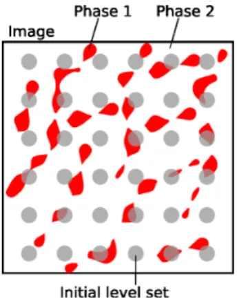
must be specified. The initial guess for the level set surface depends on the structure of the image. For a successful segmentation of an image presenting disjoint regions, the initial level set will be a family of surfaces located within each region. The location and number of the surfaces need to be specified depending on the input image. For intricate structures, a uniform layout of small circles spaced adequately (depending on the size of the detail to be captured) is chosen as the initial level set guess (see figure 3).
Figure 3: Initial level set guess in the case of intricate objects.
The level set solution is calculated to subpixel precision [76], and interpolated lin-early at pixel level which means that the interface can be located inside a pixel whose value is strictly positive or negative, depending on his neighbors (see figure 4). This can be achieved provided that the terms in eq (2) are sufficiently smooth. The processing time of the segmentation is influenced by the surface area of the evolving front and the distance the front has to travel, so that the initial conditions and convergence parameters must be chosen carefully. The output level set “image” constitutes the input geometry for the X-FEM problem. Figure 1 presents schematically the path from an acquired image to the input for an X-FEM analysis.
3 The eXtended Finite Element Method
The X-FEM is an extension of the finite element method (FEM) that was developed from the need to improve the FEM approach for problems with complex geometries. In contrast to classical finite elements, X-FEM does not require the mesh to conform the geometry. Instead, a regular mesh is constructed for the domain of interest and the pres-ence of internal boundaries (cracks, inclusions) is taken into account in the formulation of the finite elements at the corresponding locations. The X-FEM approximation of the displacement field, u, over an element is given by:
u(x)|Ωe = n ∑ α=1 Nα uα+ ne ∑ β=1 aαβ φβ(x) (4)
Figure 4: Subpixel precision of the location of the iso-zero
where the approximation can be divided into a classical one that depends only on the shape functions Nα(x) and classical degrees of freedom (dofs in the following) uα, and an enriched one that depends on enrichment functions φβ(x) and enriched dofs aαβ.
Those functions prevent poor rates of convergence due to the non-conformity of the approximation. The additional degrees of freedom are only added at the nodes whose support is split by the interface, which means that typically only a few of them are added. For material interfaces, the enrichment function φβ(x) is continuous and its derivatives
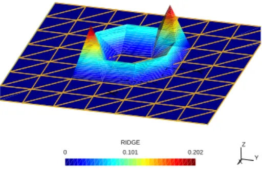
across the interfaces are discontinuous. In this paper, the following enrichment function is considered [59]: φu(x) =∑ α |ϕα|Nα(x)− ∑ α ϕαNα(x) (5)
where ϕα is the signed-distance function to the interface evaluated at the vertex of
node α (see Figure 5 for the example of a plate with a circular inclusion).
If locally the mesh conforms to the material interface, then no enrichment is added to the displacement field. A modified Gauss quadrature scheme described in [56] is used to integrate the weak form, as the gradient of the enriched part of the approximation is discontinuous. The number of integration points over each subdomain is chosen so that the integration is ’exact’. Finally, note that a linear approximation of the displacement field will be considered through this paper. The main advantage of this function over the one proposed in [58] is that the classical finite element convergence rate is preserved [58, 57, 61]. Finally, note that the so called ’corrected X-FEM’ approach could be used in order to remove the need of blending elements when using the abs enrichment function [58]. Alternatively, approaches based on Nitsche’s method [77, 78] or Lagrange multipliers [60, 79] can be used for the treatement of material interfaces.
Z Y X RIDGE 0.101 0.202 0
Figure 5: Illustration of the Ridge function for the case of a square plate with a circular inclusion in its center.
4 X-FEM and Level sets coupling
Any digital image is an implicit grid, each pixel representing the unit in terms of ge-ometry and information content. The level set information corresponding to an image constructed by segmentation inherits of this grid since the data are provided at pixel level - (see figure 6a). However, by contrast to a binarized images, the material interface does not match the voxel boundaries: it is interpolated linearly inside the cut elements. The next step is to define the discretization of the boundary value problem. Of course, a mesh based on the pixel scale can be constructed but it may not be relevant for the treatment of the problem. This actually leads to very large meshes that are computa-tionally expensive. The X-FEM allows to overcome this limitation, as it does not require a conforming mesh: A regular mesh whose scale is not dictated by the pixel size can thus be constructed (see figure 6b in the case of a circular inclusion). The pixel based level set informations are projected on this coarse mesh in order to embed the image information. This approach leads to very simple structured meshes that take into ac-count the geometrical features by mean of the level set and X-FEM enrichments. An improved version of this approach has already been proposed by Prabel et al. [80]. This approach consists in representing the levelset on a different mesh than the one used for the mechanical approximation. This allows to partially uncouple geometry and approxi-mation, as the levelset still has to be projected on the mechanical mesh at computational time. Another approach was also proposed in the context of image-based computations in [81] by mean of an adapative refinement of the mesh of the iso-surface in order to make its size sufficiently small. Another approach has been considered hereunder by taking advantage of the structured nature of the image grid, and combining it with a quadtree (octree in 3D) hierarchy of the mesh [82]. This approach allows a fine (but non-conforming) representation of the geometry near the interface (pixel sized elements)
and a coarser one in less critical area (see figure 6c). As in the former case, the pixel level-set informations are projected on the octree grid in order to embed the geometrical informations. Finally, note that it is possible to combine the two approaches, in order to take advantage of the quadtree hierarchy of the mesh but with the ability to work with fine levels that are unrelated to the pixel size (see figure 6d). Note that the projec-tion of the pixel-based level-set on the computaprojec-tional mesh will inevitably lead to some geometrical approximations of the interface location, except in the case of pixel-based computational meshes (see zoom on the interface in figure 6b). Finally, remark that a nonconforming mesh refinement could be used near the material interfaces by mean of a mesher. This would probably lead to results with an accuracy similar to the octree case. However, the approach would be less efficient as a high number of projections should be required in order to define the level-set field on this new mesh.
To illustrate the effect of de-refinement on the sample geometry, consider the image depicted in figure 7a. It is segmented using the approach presented above, and the corresponding level set (on a pixel-sized mesh) is presented in figure 7b (note that for clarity, the mesh outline was omitted). Now, the mesh is uniformly de-refined from its initial 2×2562triangular elements to a 2×162 mesh. As expected, due to the piece-wise linear approximation of the level set linked to the mesh resolution, geometrical detail is lost (e, f) for the coarsest meshes, while it remains accurate for sensible mesh (b, c, d).
5 Homogenization problem
The materials which are considered in this paper do not exhibit a regular microstruc-ture. Therefore their representative volume element (RVE) as well as the homogenization method have to be defined. The determination of the size of the RVE can be performed using several approaches [83, 71, 84], which rely on the solution of the homogenization problem on samples of different sizes. Let V be such a sample, its apparent properties correspond to the constitutive relation between the macroscopic stress Σ and the macro-scopic strain E. These macromacro-scopic quantities are defined by a spatial averaging over the sample of the corresponding microscopic fields σ and ε:
Σ =⟨σ⟩ = 1 V ∫ V σ dV E =⟨ε⟩ (6)
Since the materials studied here cannot be considered as periodic media, their ap-parent properties are computed using an homogenization scheme with uniform boundary conditions. Classically two sets of boundary conditions may be used [85], namely kine-matic uniform boundary conditions and stress uniform boundary conditions (denoted KUBC and SUBC in the following):
KUBC: u = E.x on ∂V (7)
Figure 6: a. Pixel-based mesh; b. uniformly de-refined mesh, 1 element for 4× 4 pixels (note the degradation of the geometry); c. Octree mesh with maximum geo-metrical accuracy near the interface (1 element for 1 pixel); d. Octree with coarse accuracy near the interface (1 element for 2× 2 pixels here).
a. b. c.
d. e. f.
Figure 7: a. detail of sample in Fig.1a. and two phase representation using the Level set sign in a pixel based X-FEM mesh illustrating the changes in the morphology of the Level set with the decrease of the uniform mesh refinement : b. 2×2562, c. 2× 1282, d. 2× 642, e. 2× 322, f. 2× 162
It follows that the field equations of the homogenization problem to be solved in V are (the small strain operator is denoted grads) :
divσ = 0 σ = C : ε ε = grads(u) (9)
completed with the boundary conditions (7) or (8) depending on the the data is E or Σ respectively. In the case of linear elasticity, this problem is linear and the apparent properties are obtained from the solutions of 6 independent loadings in 3D, corresponding to a unit E or Σ.
6 Numerical examples
The numerical examples will be divided in two parts: First, some validation examples to assess the accuracy of the proposed approach by mean of comparison with previously published papers. Then, three dimensional qualitative results are presented to illustrate the use of this approach in 3D.
6.1 Metallic-ceramic Composite
In order to validate the method presented above, consider a 2D reference example pub-lished in the literature. The effective properties for a sample of a ceramic-metallic composite 24% TiC/stellite obtained by homogenization and FE have been reported in [75]. The two phases are assumed isotropic and their mechanical properties are given in Table 1.
The sample is reproduced in figure 1a, and the resolution of the reference greyscale image is 256× 256 pixels. First, the level set data are obtained for this resolution, using
Properties of phases Young’s modulus (GPa) Poisson’s ratio
Stellite (nickel-based alloy) 183 0.3
TiC (carbide) 447 0.19
Effective properties [75] ∼ 226
-Table 1: Material properties for TiC and stellite.
a threshold level set filter based on the image intensity (lower threshold 100, upper threshold 255). The corresponding full-size level set is presented in figure 1b. Second, the X-FEM mesh is constructed, embedding the level set informations. The following mesh resolutions were considered: 2× 162, 2× 322, 2× 642, 2× 1282 and 2× 2562 triangular elements. The calculations are carried out on a the whole sample which is therefore considered as representative volume element (RVE) as in the paper from which it is taken from [75]. The reported effective value for the Young’s modulus of the TiC/stellite composite is approximately 226 GPa [75]. The results obtained in this study, for the different meshes considered are listed in Table 2.
Mesh size (# of elements) 2× 162 2× 322 2× 642 2× 1282 2× 2562 Poisson’s ratio 0.273 0.275 0.276 0.276 0.277 Young’s modulus (MPa) 234.5 232.5 233.6 233.5 232.8
Table 2: Effective material properties for the TiC/stellite alloy for various mesh resolutions.
The relative error between the results obtained for the coarsest mesh and the pixel based mesh is 0.7%, so even coarse meshes approximate accurately the global effective properties of the composite. The Young’s modulus values are at best 2.7% away from the reported value. The stiffness decrease induced by the mesh refinement is counteracted by the geometrical changes introduced by the embedding of the level set data in the mesh. The coarser the mesh the less geometrical details are captured therefore the overall domain occupied by the hard-phase decreases. The geometrical differences between the present model and the unit-cell based FE model used in [75] may account for the small difference in the overall stiffness results.
The distributions of the micro-stresses are in agreement in all the simulations (see figure 8). However, if the micromechanical fields of the structure are of interest, an appropriately refined mesh is needed in order to capture the stress concentrations at the interface between materials. As seen in figure 8a, the mesh coarseness gives quite a fragmented map of the Von Mises stress. In contrast, a satisfactory stress distribution is obtained using a mesh of 2× 1282 elements (see figure 8c). The mesh refinement actually improves the smoothness of the material interface, as well as the accuracy of the numerical approximation of the mechanical fields.
Figure 8: Von Mises stresses corresponding to the shearing micro-mode for different mesh sizes: a. 2× 162, b. 2× 322, c. 2× 1282
6.2 Fiber reinforced composite
As a second validation example, consider the homogenization of a fiber reinforced com-posite whose microstructure is shown in figure 9a: This image was extracted from [86] then segmented. The matrix and fibers are respectively made of epoxy and graphite. The resolution of the image is 512× 512 pixels. The material properties (assumed linear elastic) associated with the two phases are listed in Table 3, and results are compared with [86]. a. b. c. 0 0.6 1.15 St res s ( V o n M is es ) M P a
Figure 9: a. Idealized representation of the fiber-reinforced composite (512×512 pixels); b. Iso-zero of the Level set (material interface) for a sub-region (128× 128 pixels); c. Von Mises stresses corresponding to the shearing micro-mode (mesh size 2× 642 elements).
In addition to determining the effective properties of the structure, the question of the size of the RVE arises. Following the method described in [71], subdivisions of
Properties of phases Transverse Young’s modulus (GPa) Transverse shear modulus
Fibers (graphite) 7.6 2.6
Matrix (epoxy) 5.5 1.96
Table 3: Material properties for the fiber reinforced composite (2D plane strain problem).
the original sample are considered and the effective properties are determined for each sample. Regular subdivisions of the image in 4, 16, and 64 samples are analyzed, and the pixel based level set data is obtained using a threshold level set filter based on the image intensity (lower threshold 50, upper threshold 255).
The final mesh resolution was chosen such that the regular grid of element size is 4×4 pixels in the original sample as well as in all the subsamples. The iso-zero of the level set (surface ratio 1/16) is presented in figure 9b, along with the shearing micro-stresses (Von Mises) for the same sample, in figure 9c. As mentioned, we considered the plane strain assumption for all the simulations and compared our results with previously reported ones. In [86], the problem was solved under the generalized plane strain assumption, and the effective material properties were expressed through selective components of the stiffness matrix C (C11,C22, C33). The discrepancy between the present results and the reference ones is below 3% (C11: 2.32%, C22: 2.14%, C33: -2.86%). Data are presented in figure 10a, and it was found that the homogenized material has an almost isotropic behaviour (up to 99%). C11 C22 C33 Component 0 5 10 15 Stiffness (MPa) Zeman Original Avg. 1/4 samples Avg. 1/16 samples Avg. 1/64 samples
Figure 10: Comparison between the results reported by Zeman and Sejnoha [86] and the results obtained in this study (kinematic homogenization).
6.3 2D octree-based computations
As presented in section 4, four approaches can be considered for the resolution of the boundary value problem. In the two last examples, the computational grid was an uniform de-refinement of the pixel-based grid (see figure 6b for the case where one finite element corresponds to 4× 4 pixels). In the following example, an octree hierarchy is combined with a selective de-refinement of the pixel-based grid (see figures 6c and 6d). The objective of the following examples is to study the influence of this approach on the accuracy and computational cost. Note that the use of a quadtree/octree mesh in the context of X-FEM leads to extra difficulties when hanging nodes are enriched. In this work, the mesh was defined so that it was ensured that none of the hanging nodes could be enriched. Otherwise, different approaches have been proposed to allow enriched hanging nodes [87, 88, 89].
6.3.1 Fiber reinforced composite
In this example the whole specimen depicted in figure 9a is considered, and the mesh size is set to the pixel size for the elements close to the interface. Away from this layer of elements, the mesh is de-refined. In order to maintain a good accuracy of the numerical scheme, the coarsening procedure ensures that the level of refinement between one element and it’s neighbors cannot have more than one generation difference. The resulting computational mesh is depicted in figure 11: 50% of the initial dofs have been saved thanks to this procedure, which ensures good compromise between accuracy and computational cost.
Figure 11: Computational octree mesh.
The specimen behavior is homogenized by mean of KUBC boundary conditions, and the results compare favorably with those depicted in figure 10a. More precisely, the discrepancy between the octree approach and those obtained in section 6.2 using homogeneous derefinment is below 0.05% (see table 4).
In this case, the number of dofs is higher than with the uniform de-refinement, but the geometrical accuracy is maximal. As seen above, the influence of the geometrical
dofs Error on C11 Error on max(σ
V M) (Shear mode)
Pixel mesh 590592 Ref. Ref.
Octree pixel mesh 270238 0.007 % 0.28 %
Uniform 4× 4 47374 0.03 % 14 %
Octree 4× 4 45650 0.031346 % 14 %
Table 4: Comparison between uniform de-refinement and octree de-refinement (fiber re-inforced composite). Octree pixel mesh means that the finest level of the octree corresponds to the pixel size; Octree 4×4 means that the finest level corresponds to 4× 4 pixels.
representation have a small influence on the homogenized behavior. However, the influ-ence of the geometry can be seen when dealing with the local stress field in the specimen: the error on the Von-Mises stress tensor increases by 14% when uniformly derefining the mesh whereas it remains below 0.3% with the selective de-refinement.
As a last application, the octree procedure is reapplied, but the finest grid size is no-longer equal to the pixel size. In this case, the smaller grid size corresponds to a set of 4× 4 pixels, as in section 6.2. The number of degrees of freedom drops now by only 4% with respect to the uniformly de-refined mesh (92% w.r. to pixel-bases mesh), and the results are comparable to the uniformly de-refined case.
6.4 Metallic-ceramic composite
In the last example, the large number of small heterogeneities did not enable to exploit the advantages of the octree approach. This is why the Metallic-ceramic composite example (see section 6.1) is now also considered in the framework of the octree approach. As in the last example, four meshes have been studied: (i) pixel-based mesh, (ii) octree mesh with fine level of pixel size, (iii) 4× 4 pixels based-mesh and (iv) octree mesh with fine level of 4× 4 pixels size. Those four meshes are depicted in figure 12. As in the last section, the number of dofs, the error on the C11 term of the homogenized behavior and the error on the maximal Von-Mises stress in shear mode are compared in table 5. In this case, the octree approach allows to save between 78 and 96 % of the dofs, depending on the level of de-refinement. It is even possible to save 45% of dofs with respect to the uniformly de-refined mesh (with a similar accuracy). As in the previous example, the influence of the geometrical representation of the sample has a great influence on the local stresses.
6.5 3D octree-based computations
As a last example and to demonstrate the capabilities of the method, we present an application of the octree approach in the 3D setting. A more extensive study of the 3D case, with comparison with voxel-based approaches will be carried out in a forthcom-ing paper. Consider the three-dimensional micro-structure depicted in figure 13 which consists of an extruded bio-polymer [90]. The acquisition of was done using synchrotron
(i) (ii)
(iii) (iv)
Figure 12: Comparison between uniform derefinment and octree derefinment (metallic-ceramic composite) ((i): the mesh has been omitted for clarity)
dofs Error on C11 Error on max(σV M) (Shear mode)
Pixel mesh 547850 Ref. Ref.
Octree pixel mesh 107378 0.04 % 0.17 %
Uniform 4× 4 37818 0.16 % 31.4 %
Octree 4× 4 22040 0.14 % 31.4%
Table 5: Comparison between uniform derefinment and octree derefinment (metallic-ceramic composite)
facilities (ESRF, Grenoble). Only a 64× 64 × 64 voxels3 subset of the initial image is considered here, as depicted in figure 14a. The material is considered as linear elastic with Young’s modulus 5.8 GPa and Poisson’s ratio 0.35. An octree adapted mesh is con-sidered in order to keep maximal geometrical accuracy and leads to the computational mesh presented in figure 14b. This mesh is geometrically refined close to the interfaces, and is gradually de-refined away from the interface. The domain is subjected to an uni-axial tension macroscopic mode along the x axis by mean of an imposed displacements (KUBC), and the results are presented in figure 15 for both displacement and stresses.
Figure 13: Segmentation of the full sample
7 Discussion and conclusions
In this paper, we presented advantages of using a method coupling X-FEM and level set segmentation in order to solve homogenization problems for structures represented by digital images. This approach offers a direct way to treat problems involving complex micro-structures, taking advantage of the versatility of the two approaches. Level sets allow the segmentation of complex shapes and leads to an accurate input of the geometry in X-FEM. In contrast with voxel-based approaches, the boundaries of the interfaces are C0, independently of the mesh size. Thus, no additional smoothing is required to keep regular boundaries.
The X-FEM then allows to solve the homogenization problem on a non-conforming mesh by means of suitable enrichments. The definition of the level set at subpixel precision allows a very fine geometrical representation of the material interface. However during the X-FEM computations, the geometrical data were provided by the nodal
a. b.
Figure 14: 3D example: a. Matter part of the levelset; b. Level set on the computational mesh
a. b.
values of the level-set on the computational mesh. Therefore, the computational mesh controls the geometrical representation, which will be maximal if a pixed-based mesh is used. Unfortunately, this mesh leads to a large computational cost. To overcome this limitation, two alternatives were proposed: First, the use of an uniformly de-refined meshes and second the use of an octree adapted mesh. The accuracy of these approaches has been studied in this paper.
The first approach allows the user to reduce dramatically the computational cost. However, it does not allow to adapt locally the mesh size to the problem at hand, and may lead to poor geometrical description. In the second approach, the accuracy is maximal near the interfaces (where elements with a pixel size are used), and the computational cost can be optimized by coarsening the mesh away from the interfaces. In was shown in the numerical examples that for a given geometrical accuracy, the octree-based approach lead to results close to those obtained with uniformly de-refined meshes, but with a much smaller computational cost. Therefore, the X-FEM and level set computational approach with geometrically adaptive octree meshes presented here turns out to be an efficient method for image-based modeling.
Yet, the de-refinement of the mesh was purely geometric and did not take into ac-count the accuracy of the mechanical fields. Error estimation procedures have already been proposed in the context of X-FEM for cracks [91, 92, 93, 94, 95] and material inter-faces [94]. Such an approach should be considered to define the mesh size. Furthermore, the mesh size is driven mainly by the size of the geometrical features, which still leads to expensive models. The key idea is to separate geometrical and mechanical models in order to keep smaller numerical models without any geometrical loss. Strategies have already proposed in this line in [42], in the case of holes and with voxelized boundaries. Work is currently in progress, based on advanced integration techniques developed in [61].
Acknowledgments I.Ionescu gratefully acknowledges the financial support from the French Minist`ere d´el´egu´e `a l’Enseignement sup´erieur et `a la Recherche.
The authors would like to thank Dr. Sofiane Guessasma for providing them biopolymer datas.
Support of INRA and CNRS are acknowledged through project PEPS ’SIFRAGAM’.
References
[1] D. Marr and E. Hildreth. Theory of edge detection. Proceedings of the Royal Society of London. Series B. Biological Siences, pages 187–217, 1980.
[2] D.L. Phan, C.Xu, and J. Price. A survey of current methods in medical image segmentation. Annual Review of Biomedical Engineering, 1998.
[3] S. Beucher and F. Meyer. The morphological approach to segmentation: the water-shed transformation. Mathematical Morphology in Image Processing, pages 433–481, 1993.
[4] R. Malladi, J.A. Sethian, and B.C. Vemuri. A topology independent shape modeling scheme. In SPIE Conf. on Geometric Methods, Comp. Vision II, volume 2031, pages 246–258, 1994.
[5] V. Caselles, R. Kimmel, and G. Sapiro. Geodesic active contours. In Proc. IEEE Intl. Conf. on Comp. Vis., pages 649–699, 1995.
[6] S. Kichenassamy, A. Kumar, P.J. Olver, A. Tannenbaum, and A. J. Yezzi. Gradient flows and geometric active contour models. In IEEE Int. Conf. on Computer Vision, pages 810–815, 1995.
[7] D. Cremers, M. Rousson, and R. Deriche. A review of statistical approaches to level set segmentation: integrating color, texture, motion and shape. Int. J. of Computer Vision, 72(2):195–215, 2007.
[8] H. Singh, A.M. Gokhale, Y. Mao, and J.E. Spowart. Computer simulations of real-istic microstructures of discontinuously reinforced aluminum alloy (dra) composites. Acta Materialia, 54(8):2131 – 2143, 2006.
[9] H. Singh, A.M. Gokhale, A. Sreeranganathan, Y. Mao, S.I. Lieberman, and S. Tamirisakandala. Computer simulations of realistic partially anisotropic mi-crostructures statistically similar to real mimi-crostructures. Computational Materials Science, 44(4):1050 – 1055, 2009.
[10] N. Chawla, R.S. Sidhu, and V.V. Ganesh. Three-dimensional visualization and microstructure-based modeling of deformation in particle-reinforced composites. Acta Materialia, 54(6):1541 – 1548, 2006.
[11] M. Groeber, S. Ghosh, M. D. Uchic, and D. M. Dimiduk. A framework for au-tomated analysis and simulation of 3d polycrystalline microstructures.: Part 1: Statistical characterization. Acta Materialia, 56(6):1257 – 1273, 2008.
[12] M. Groeber, S. Ghosh, M. D. Uchic, and D. M. Dimiduk. A framework for auto-mated analysis and simulation of 3d polycrystalline microstructures. part 2: Syn-thetic structure generation. Acta Materialia, 56(6):1274 – 1287, 2008.
[13] P.G Young, T.B.H Beresford-West, S.R.L Coward, B Notarberardino, B Walker, and A Abdul-Aziz. An efficient approach to converting three-dimensional image data into highly accurate computational models. Philosophical Transactions of the Royal Society A: Mathematical, Physical and Engineering Sciences, 366(1878):3155– 3173, 2008.
[14] M. Viceconti, L. Bellingeri, L. Cristofolini, and A. Toni. A comparative study on different methods of automatic mesh generation of human femurs. Medical Engi-neering & Physics, 20(1):1 – 10, 1998.
[15] P.J. Frey. Generation and adaptation of computational surface meshes from discrete anatomical data. International Journal for Numerical Methods in Engineering, 60(6):1049–1074, 2004.
[16] D. Ulrich, B. van Rietbergen, H. Weinans, and P. Regsegger. Finite element analysis of trabecular bone structure: a comparison of image-based meshing techniques. Journal of Biomechanics, 31(12):1187 – 1192, 1998.
[17] S. Youssef, E. Maire, and R. Gaertner. Finite element modelling of the actual structure of cellular materials determined by x-ray tomography. Acta Materialia, 53(3):719 – 730, 2005.
[18] K. Madi, S. Forest, M. Boussuge, S. Gailligue, E. Lataste, J.-Y. Buffire, D. Bernard, and D. Jeulin. Finite element simulations of the deformation of fused-cast refrac-tories based on x-ray computed tomography. Computational Materials Science, 39(1):224 – 229, 2007.
[19] Z. Yu, M. J. Holst, and J. A. McCammon. High-fidelity geometric modeling for biomedical applications. Finite Elements in Analysis and Design, 44(11):715 – 723, 2008.
[20] A. Fedorov and N. Chrisochoides. Tetrahedral mesh generation for non-rigid regis-tration of brain mri: Analysis of the requirements and evaluation of solutions. In 17th International Meshing Roundtable. Springer Verlag, 2008.
[21] H.J. Kim and C.C. Swan. Voxel-based meshing and unit-cell analysis of textile com-posites. International Journal for Numerical Methods in Engineering, 56(7):977– 1006, 2003.
[22] J.H. Keyak, J.M. Meagher, H.B. Skinner, C.D. Mote, and Jr. Automated three-dimensional finite element modelling of bone: a new method. Journal of Biomedical Engineering, 12(5):389 – 397, 1990.
[23] S.J. Hollister and N. Kikuchi. Homogenization theory and digital imaging: a basis for studying the mechanics and design principles of bone tissue. Biotechnology and Bioengineering, 43(7):586–596, 1994.
[24] L. L. Mishnaevsky Jr. Automatic voxel-based generation of 3d microstructural fe models and its application to the damage analysis of composites. Materials Science and Engineering: A, 407(1-2):11 – 23, 2005.
[25] P. Arbenz, G.H. van Lenthe, U. Mennel, R. M¨uller, and M. Sala. A scalable multi-level preconditioner for matrix-free µ-finite element analysis of human bone struc-tures. International Journal for Numerical Methods in Engineering, 73(7):927–947, 2008.
[26] E. Maire, A. Fazekas, L. Salvo, R. Dendievel, S. Youssef, P. Cloetens, and J.-M. Letang. X-ray tomography applied to the characterization of cellular materi-als. related finite element modeling problems. Composites Science and Technology, 63(16):2431 – 2443, 2003.
[27] P. Babin, G.D. Valle, R. Dendievel, N. Lassoued, and L. Salvo. Mechanical proper-ties of bread crumbs from tomography based Finite Element simulations. Journal of Materials Science, 40(22):5867–5873, 2005.
[28] A.C. Lewis and A.B. Geltmacher. Image-based modeling of the response of exper-imental 3d microstructures to mechanical loading. Scripta Materialia, 55(1):81 – 85, 2006.
[29] G. T. Charras and R. E. Guldberg. Improving the local solution accuracy of large-scale digital image-based finite element analyses. Journal of Biomechanics, 33(2):255 – 259, 2000.
[30] N. Takano, M. Zako, F. Kubo, and K. Kimura. Microstructure-based stress analysis and evaluation for porous ceramics by homogenization method with digital image-based modeling. International Journal of Solids and Structures, 40(5):1225 – 1242, 2003.
[31] D. L. A. Camacho, R. H. Hopper, G. M. Lin, and B. S. Myers. An improved method for finite element mesh generation of geometrically complex structures with application to the skullbase. Journal of Biomechanics, 30(10):1067 – 1070, 1997. [32] J.R. Cebral and R. L¨ohner. From medical images to anatomically accurate
fi-nite element grids. International Journal for Numerical Methods in Engineering, 51(8):985–1008, 2001.
[33] Z.L. Wang, J.C.M. Teo, C.K. Chui, S.H. Ong, C.H. Yan, S.C. Wang, H.K. Wong, and S.H. Teoh. Computational biomechanical modelling of the lumbar spine us-ing marchus-ing-cubes surface smoothened finite element voxel meshus-ing. Computer Methods and Programs in Biomedicine, 80(1):25 – 35, 2005.
[34] S. K. Boyd and R. M¨uller. Smooth surface meshing for automated finite element model generation from 3d image data. Journal of Biomechanics, 39(7):1287 – 1295, 2006.
[35] H. Moulinec and P. Suquet. A numerical method for computing the overall response of nonlinear composites with complex microstructure. Computer Methods in Applied Mechanics and Engineering, 157(1-2):69 – 94, 1998.
[36] H. Moulinec and P. Suquet. Comparison of FFT-based methods for computing the response of composites with highly contrasted mechanical properties. Physica B: Condensed Matter, 338(1-4):58 – 60, 2003.
[37] V. Vinogradov and G. W. Milton. An accelerated fft algorithm for thermoelastic and non-linear composites. International Journal for Numerical Methods in Engineering, 76(11):1678–1695, 2008.
[38] M.I. Idiart, F. Willot, Y.-P. Pellegrini, and P. Ponte Casta˜neda. Infinite-contrast pe-riodic composites with strongly nonlinear behavior: Effective-medium theory versus
full-field simulations. International Journal of Solids and Structures, 46(18-19):3365 – 3382, 2009.
[39] W Hackbusch and S A Sauter. Composite finite elements for the approximation of PDEs on domains with complicated micro-structures. Numerische Mathematik, 75(4):447–472, February 1997.
[40] F. Liehr, T. Preusser, M. Rumpf, S. Sauter, and L. Schwen. Composite finite elements for 3D image based computing. Computing and Visualization in Science, 12(4):171–188, April 2009.
[41] J. Parvizian, A. D¨uster, and E. Rank. Finite cell method. Computational Mechanics, 41(1):121–133, 2007.
[42] A. D¨uster, J. Parvizian, Z. Yang, and E. Rank. The finite cell method for three-dimensional problems of solid mechanics. Computer Methods in Applied Mechanics and Engineering, 197(45-48):3768 – 3782, 2008.
[43] K. Terada, M. Asai, and M. Yamagishi. Finite cover method for linear and non-linear analyses of heterogeneous solids. International journal for numerical methods in engineering, 58(9):1321–1346, 2003.
[44] K. Terada and M. Kurumatani. An integrated procedure for three-dimensional structural analysis with the finite cover method. International Journal for Numer-ical Methods in Engineering, 63:2102–2123, 2005.
[45] M. Kurumatani and K. Terada. Finite cover method with multi-cover layers for the analysis of evolving discontinuities in heterogeneous media. International Journal for Numerical Methods in Engineering, 79(1):1–24, 2009.
[46] I. Babuska and J. Y. Melenk. The partition of unity finite element method. Inter-national Journal for Numerical Methods in Engineering, 40(4):727–758, 1997. [47] C.A. Duarte and J.T Oden. An h-p adaptive method using clouds. Computer
Methods in Applied Mechanics and Engineering, 139(1-4):237–262, 1996.
[48] C. Duarte and J. Oden. An hp meshless Method. Numerical methods for partial differential equations, 12:673–705, 1996.
[49] T. Belytschko, R. Gracie, and G. Ventura. A review of extended/generalized finite element methods for material modeling. Modelling and Simulation in Materials Science and Engineering, 17:043001, 2009.
[50] T. Strouboulis, I. Babuˇska, and K. Copps. The design and analysis of the generalized finite element method. Computer Methods in Applied Mechanics and Engineering, 181:43–69, 2000.
[51] T. Strouboulis, K. Copps, and I. Babuˇska. The generalized finite element method. Computer Methods in Applied Mechanics and Engineering, 190(32-33):4081–4193, 2001.
[52] T. Strouboulis, L. Zhang, and I. Babuˇska. Generalized finite element method us-ing mesh-based handbooks: application to problems in domains with many voids. Computer Methods in Applied Mechanics and Engineering, 192(28-30):3109–3161, 2003.
[53] T. Strouboulis, L. Zhang, and I. Babuˇska. p-version of the generalized fem us-ing mesh-based handbooks with applications to multiscale problems. International Journal for Numerical Methods in Engineering, 60(10):1639–1672, 2004.
[54] C. A. Duarte and D. J. Kim. Analysis and applications of a generalized finite ele-ment method with global-local enrichele-ment functions. Computer Methods in Applied Mechanics and Engineering, 197:487–504, Jan 2008.
[55] T. Belytschko and T. Black. Elastic Crack Growth in Finite Elements with Min-imal Remeshing. International Journal for Numerical Methods in Engineering, 45(5):601–620, 1999.
[56] N. Mo¨es, J. Dolbow, and T. Belytschko. A finite element method for crack growth without remeshing. International Journal for Numerical Methods in Engineering, 46:131–150, 1999.
[57] G. Legrain, N. Mo¨es, and A. Huerta. Stability of incompressible formulations en-riched with X-FEM. Computer Methods in Applied Mechanics and Engineering, 197(21-24):1835–1849, 2008.
[58] N. Sukumar, D. L. Chopp, N. Mo¨es, and T. Belytschko. Modeling Holes and In-clusions by Level Sets in the Extended Finite Element Method. Comp. Meth. in Applied Mech. and Engrg., 190:6183–6200, 2001.
[59] N. Mo¨es, M. Cloirec, P. Cartraud, and J.-F. Remacle. A computational approach to handle complex microstructure geometries. Comp. Meth. in Applied Mech. and Engrg., 192:3163–3177, 2003.
[60] N. Mo¨es, E. B´echet, and M. Tourbier. Imposing dirichlet boundary conditions in the extended finite element method. International Journal for Numerical Methods in Engineering, 67(12):1641–1669, 2006.
[61] Kristell Dr´eau, Nicolas Chevaugeon, and Nicolas Mo¨es. Studied X-FEM enrichment to handle material interfaces with higher order finite element. Computer Methods in Applied Mechanics and Engineering, 199(29-32):1922–1936, 2010.
[62] C. Daux, N. Mo¨es, J. Dolbow, N. Sukumar, and T. Belytschko. Arbitrary branched and intersecting cracks with the eXtended Finite Element Method. International Journal for Numerical Methods in Engineering, 48:1741–1760, 2000.
[63] R. de Borst. Challenges in computational materials science: Multiple scales, multi-physics and evolving discontinuities. Computational Materials Science, 43(1):1 – 15, 2008. Proceedings of the 16th International Workshop on Computational Mechanics of Materials - IWCMM-16.
[64] P. Michlik and C. Berndt. Image-based extended finite element modeling of thermal barrier coatings. Surface and Coatings Technology, 201(6):2369 – 2380, 2006. [65] A.C.E. Reid, S.A. Langer, R.C. Lua, V.R. Coffman, S.-I Haan, and R.E. Garc´ıa.
Image-based finite element mesh construction for material microstructures. Com-putational Materials Science, 43(4):989 – 999, 2008.
[66] ´E. Budyn and T. Hoc. Analysis of micro fracture in human Haversian cortical bone under transverse tension using extended physical imaging. International Journal for Numerical Methods in Engineering, 82(8):940–965, 2010.
[67] J. R´ethor´e, F. Hild, and S. Roux. Shear-band capturing using a multiscale extended digital image correlation technique. Computer Methods in Applied Mechanics and Engineering, 196(49-52):5016 – 5030, 2007.
[68] J. R´ethor´e, F. Hild, and S. Roux. Extended digital image correlation with crack shape optimization. International Journal for Numerical Methods in Engineering, 73(2):248–272, 2008.
[69] J.A. Sethian. Level Set Methods: Evolving Interfaces in Geometry, Fluid Mechan-ics, Computer Vision and Materials Sciences. Cambridge Monographs on Applied and Computational Mathematics (No. 3). Cambridge University Press, 2nd edition, 1999.
[70] Mitsuhiro Kawagai, Atsushi Sando, and Naoki Takano. Image-based multi-scale modelling strategy for complex and heterogeneous porous microstructures by mesh superposition method. Modelling and Simulation in Materials Science and Engi-neering, 14(1):53–69, 2006.
[71] Toufik Kanit, Franck N’Guyen, Samuel Forest, Dominique Jeulin, Matt Reed, and Scott Singleton. Apparent and effective physical properties of heterogeneous mate-rials: Representativity of samples of two materials from food industry. Computer Methods in Applied Mechanics and Engineering, 195(33-36):3960–3982, 2006. [72] H. Kumar, C.L. Briant, and W.A. Curtin. Using microstructure reconstruction to
model mechanical behavior in complex microstructures. Mechanics of Materials -Advances in Disordered Materials, 38(8-10):818–832, 2006.
[73] N. Takano, M. Zako, F. Kubo, and K. Kimura. Microstructure-based stress analysis and evaluation for porous ceramics by homogenization method with digital image-based modeling. International Journal of Solids and Structures, 40(5):1225–1242, 2003.
[74] Patrice Cartraud, Irina Ionescu, Gregory Legrain, and Nicolas Mo¨es. Image-based computational homogenization of random materials using level sets and x-fem. In 5th. European Congress on Computational Methods in Applied Sciences and En-gineering (ECCOMAS 2008) - 8th. World Congress on Computational Mechanics (WCCM8), 2008.
[75] D. Golanski, K. Terada, and N. Kikuchi. Macro and micro scale modeling of thermal residual stresses in metal matrix composite surface layers by the homogenization method. Computational Mechanics, 19(3):188–202, 1997.
[76] Ibanez L., Schroeder W., Ng L., and Cates J. The ITK Software Guide. Kitware, Inc., 2005 edition, 2005.
[77] J. Nitsche. ¨Uber ein Variationprinzip zur l¨osung von Dirichlet-Problem bei Verwen-dung von Teilr¨aumen, die keinen Randbedingungen unterworfen sind. Abh. Math. Sem. Univ. Hamburg, 36:9–15, 1971.
[78] Anita Hansbo and Peter Hansbo. A finite element method for the simulation of strong and weak discontinuities in solid mechanics. Computer Methods in Applied Mechanics and Engineering, 193(33-35):3523–3540, August 2004.
[79] E. B´echet, N. Mo¨es, and B. Wohlmuth. A stable lagrange multiplier space for the stiff interface conditions within the extende finite element method. International Journal for Numerical Methods in Engineering, 78(8):931–954, 2009.
[80] B. Prabel, A. Combescure, A. Gravouil, and S. Marie. Level set X-FEM non-matching meshes: application to dynamic crack propagation in elasticplastic me-dia. International Journal for Numerical Methods in Engineering, 69(8):1553–1569, 2007.
[81] E. Pierres, M.C. Baietto, A. Gravouil, and G. Morales-Espejel. 3d two scale x-fem crack model with interfacial frictional contact: Application to fretting fatigue. Tribology International, 43(10):1831 – 1841, 2010. 36th Leeds-Lyon Symposium Special Issue: Multi-facets of Tribology.
[82] P. Frey and P. George. Mesh Generation: Application to Finite Elements. Hermes Science Publishing Ltd;, 2000.
[83] T. Kanit, S. Forest, I. Galliet, V. Mounoury, and D. Jeulin. Determination of the size of the representative volume element for random composites: statistical and numerical approach. International Journal of Solids and Structures, 40(13-14):3647–3679, 2003.
[84] M. Ostoja-Starzewski. Material spatial randomness: From statistical to represen-tative volume element. Probabilistic Engineering Mechanics, 21(2):112 – 132, 2006. [85] P. Suquet. Elements of homogenization for inelastic solid mechanics. In E. Sanchez-Palencia and A. Zaoui, editors, Homogenization Techniques for Composite Media,
volume 272 of Lecture Notes in Physics, pages 193–278. Springer-Verlag, Berlin, 1985.
[86] J. Zeman and M. Sejnoha. Numerical evaluation of effective elastic properties of graphite fiber tow impregnated by polymer matrix. Journal of the Mechanics and Physics of Solids, 49(1):69–90, 2001.
[87] A. Tabarraei and N. Sukumar. Extended finite element method on polygonal and quadtree meshes. Computer Methods in Applied Mechanics and Engineering, 197(5):425–438, 2008.
[88] G. Legrain, R. Allais, and P. Cartraud. On the use of the extended finite element method with quatree/octree meshes. International Journal for Numerical Methods in Engineering, Submitted:n/a, 2010.
[89] A. Alizada and T. P. Fries. Cracks and crack propagation with xfem and hanging nodes in 2d. In IV European Conference on Computational Mechanics, 2010. [90] S. Guessasma, P. Babin, G. Della Valle, and R. Dendievel. Relating cellular
struc-ture of open solid food foams to their young’s modulus: Finite element calculation. International Journal of Solids and Structures, 45(10):2881 – 2896, 2008.
[91] M. Duflot and S. Bordas. A posteriori error estimation for extended finite elements by an extended global recovery. International Journal for Numerical Methods in Engineering, 76(8):1123–1138, 2008.
[92] S. Bordas and M. Duflot. Derivative recovery and a posteriori error estimate for extended finite elements. Computer Methods in Applied Mechanics and Engineering, 196(35-36):3381–3399, 2007.
[93] J. J. R´odenas, O. A. Gonz`alez-Estrada, J. E. Taranc´on, and F. J. Fuenmayor. A recovery-type error estimator for the extended finite element method based on singular+smooth stress field splitting. International Journal for Numerical Methods in Engineering, 76(4):545–571, 2008.
[94] R. Allais, G. Legrain, and P. Cartraud. Comparison of two approaches for error estimation with X-FEM. In IV European Conference on Computational Mechanics, 2010.
[95] C. Hoppe, S. Loehnert, P. Wriggers, and E. Stein. Error estimation within the extended finite element analysis of cracks. In IV European Conference on Compu-tational Mechanics, 2010.