HAL Id: hal-00296500
https://hal.archives-ouvertes.fr/hal-00296500
Submitted on 20 Mar 2008
HAL is a multi-disciplinary open access
archive for the deposit and dissemination of
sci-entific research documents, whether they are
pub-lished or not. The documents may come from
teaching and research institutions in France or
abroad, or from public or private research centers.
L’archive ouverte pluridisciplinaire HAL, est
destinée au dépôt et à la diffusion de documents
scientifiques de niveau recherche, publiés ou non,
émanant des établissements d’enseignement et de
recherche français ou étrangers, des laboratoires
publics ou privés.
version of the new dynamics Unified Model
P. J. Telford, P. Braesicke, O. Morgenstern, J. A. Pyle
To cite this version:
P. J. Telford, P. Braesicke, O. Morgenstern, J. A. Pyle. Technical Note: Description and assessment of
a nudged version of the new dynamics Unified Model. Atmospheric Chemistry and Physics, European
Geosciences Union, 2008, 8 (6), pp.1701-1712. �hal-00296500�
www.atmos-chem-phys.net/8/1701/2008/ © Author(s) 2008. This work is distributed under the Creative Commons Attribution 3.0 License.
Chemistry
and Physics
Technical Note: Description and assessment of a nudged version of
the new dynamics Unified Model
P. J. Telford, P. Braesicke, O. Morgenstern, and J. A. Pyle University of Cambridge, Cambridge NCAS-Climate, UK
Received: 4 October 2007 – Published in Atmos. Chem. Phys. Discuss.: 27 November 2007 Revised: 26 February 2008 – Accepted: 28 February 2008 – Published: 20 March 2008
Abstract. We present a “nudged” version of the Met Office general circulation model, the Unified Model. We constrain this global climate model using ERA-40 re-analysis data with the aim of reproducing the observed “weather” over a year from September 1999. Quantitative assessments are made of its performance, focusing on dynamical aspects of nudging and demonstrating that the “weather” is well simulated.
1 Introduction
The ability to mimic the real state of the atmosphere, the “weather”, in a climate model is useful for studying pro-cesses on short time scales for which monthly means contain only a limited amount of information. Newtonian relaxation or “nudging” is a method that adjusts dynamical variables of general circulation models (GCM) towards meteorolog-ical re-analysis data, providing a realistic representation of the weather.
Jeuken et al. (1996) were the first to consider applying the technique to the validation of GCMs, adding nudging to the ECHAM GCM. This remains the most complete description of a nudged model, though others exist, including the LMDZ (Hauglustaine et al., 2004), GISS (Schmidt et al., 2006) and CCSR/NIES AGCM (Takemura et al., 2000) models. The technique has been widely adopted to study processes where capturing the daily variability of phenomena is important. Examples include examining the behaviour of chemical trac-ers (van Aalst et al., 2004), and studying the properties of clouds (Dean et al., 2006).
The climate model which we nudge is the Met. Office GCM, the Unified Model (henceforth the UM) (Staniforth et al., 2005). There have been applications of the nudging
Correspondence to: P. J. Telford
technique in earlier versions of this model, to study clouds (Flowerdew et al., 20081) and to include a realistic quasi bi-ennial oscillation (Pyle et al., 2005). We describe the first implementation of the nudging technique to the new non-hydrostatic version of the UM, the “New Dynamics” UM, and evaluate the performance of the system for a 12 month integration starting in September 1999.
After a brief description of the model, we provide a quan-titative assessment of its performance with respect to the ERA-40 re-analysis data. The RMSE, bias and correlations in space and time between the model and the ERA-40 data are calculated, with and without nudging, for variables that are directly adjusted by the nudging and variables adjusted indirectly. After varying a few key parameters we conclude by considering future prospects for the model.
2 Model description
The Model is based upon version 6.1 of the UM (Staniforth et al., 2005). The dynamical prognostic variables adjusted by nudging are potential temperature, θ , zonal wind, u, and meridional wind, v. The configuration used has
– a horizontal resolution of 3.75◦×2.5◦in longitude and
latitude.
– 60 hybrid height levels in the vertical, from the surface up to a height of 84 km.
– a dynamical time-step of 20 min.
The sea surface temperatures and sea ice coverage are pre-scribed from the HADISST dataset (Rayner et al., 2002). The version of the model used was known to have temper-ature biases, the most notable being a warm bias in the lower
1Flowerdew, J., Lawrence, B. N., and Andrews, D.: The use
of nudging and feature tracking to evaluate climate model cloud, Climate Physics, in review, 2008.
stratosphere, especially over the poles, and around the trop-ical tropopause. The initial conditions are taken from the default climate integration file.
We add a module that reads global re-analysis data and “nudges” the model towards it. The re-analysis data used here is from the ECMWF ERA-40 dataset (ECMWF, 1996; Uppala et al., 2005). Although there are some weaknesses in the ERA-40 analysis, such as an overly strong Brewer-Dobson Circulation (Uppala et al., 2005), they have been widely used (Jeuken et al., 1996; Hauglustaine et al., 2004) and are adequate to assess the performance of the nudging technique.
2.1 Data utilised
The ECMWF ERA-40 re-analysis data is used to constrain the model. It is available at six hourly intervals on a 1◦×1◦ grid. The variables taken for nudging are
tempera-ture, T , zonal wind, u, and meridional wind, v. The ERA-40 data is pre-processed horizontally by bi-linearly interpolating on to the model grid.
At run-time the data is linearly interpolated on to the model time-steps. Previous studies indicate that there is no advantage to using more complex interpolations over these time-scales (Brill et al., 1991). No explicit truncation, like that used by Jeuken et al. (1996), is applied. The conversion to a coarser resolution and the smooth linear interpolation in time should favour slow and large scale horizontal motions, removing most “noise” from the data.
To obtain the UM prognostic variables, T is converted to θ . The variables, u, v and θ , are interpolated linearly in log-arithm of pressure, ln(P ), from the ECMWF hybrid pressure levels to the UM hybrid height levels. The orographies in the UM and ECMWF models, although based on similar data-sets, are different due to different processing procedures for different grids. These differences can be as large as hundreds of metres in the Andes and Antarctica. They can produce errors in the interpolation from the ECMWF to UM model levels due to the vertical structure of the model levels being represented differently in the two models.
A solution considered was the use of the ECMWF orog-raphy in the nudged UM model. However this would create problems; apart from the question of how to interpret a spec-tral orography in a grid-point model, it could disrupt other as-pects of the model such as orographic gravity wave drag. The errors in the interpolation occur predominantly in the lowest few model levels, which are not utilised by the nudging. The small improvement on a few levels used by the nudging was not felt to justify the problems that using the ECMWF orog-raphy would cause. Although using the Met Office analysis data (Lorenc et al., 1999) would remove any differences in orography they were not used as they are only available once a day.
2.2 Set up of the nudging
The ERA-40 data is included into the model by the addition of non-physical relaxation terms to the model equations. The rate of change in a variable, X, is obtained from
δX
δt =Fm(X) + G(Xana−X), (1)
where Fmis the rate of change in the variable due to all other
factors, Xanais the value of the variable in the ERA-40 data
and G is the relaxation parameter (Jeuken et al., 1996). As we are working in discrete time-steps this equation is imple-mented explicitly as
1X = Fmt(X) + (G1t )(Xana−X), (2)
where Fmt is the change of the variable due to all other
fac-tors over the dynamical time-step and 1t is the dynamical time-step size.
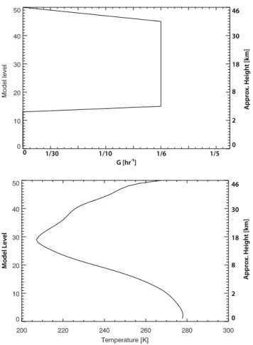
The choice of relaxation parameter, although arbitrary, is important, as if it is too small nudging is ineffective, yet too large and the model becomes unstable. The value chosen is the “natural” one of 16h−1, the time spacing of the ERA-40
data. This also lies within the range of relaxation parame-ters used by other models (Jeuken et al., 1996; Hauglustaine et al., 2004; Schmidt et al., 2006).
The variation of the relaxation parameter with UM hybrid height level is displayed in Fig. 1. The average ECMWF tem-perature, as a function of UM hybrid height level, is included for orientation. The temperature is taken from the ERA-40 data in October 1999 and interpolated onto the UM hybrid height levels.
Nudging is not applied to all levels; it is not applied on levels which utilise data from the topmost ECMWF hybrid pressure levels, or in the bottommost levels that constitute the boundary layer. This results in no nudging being applied above level 50 (∼48 km), with a linear increase in G from 0 at level 50 to its full value at level 45 (∼38 km), or below level 12 (∼2.9 km)2, with a linear increase in G from 0 at level 12 to its full value at level 15 (∼4.5 km). The effect of using different relaxation parameters and vertical ranges is discussed in Sect. 4.
3 Assessment of model performance
The model was run for a year starting from 1 September 1999. From this simulation three periods are selected for more detailed analysis; October, January and July. Dur-ing these periods a suite of statistical tools is used to deter-mine the size of any differences and correlations between the model and the ERA-40 data.
The main assessment consists of a series of comparisons of variables, including some which are nudged directly (u
2The levels are hybrid height levels and their exact values
and θ ), and some which are not (surface pressure, Ps, and
specific humidity, q). The comparison examines the size and variation of differences between the model and the ERA-40 data. In addition derived quantities, such as precipitation and vertical wind are compared. To establish that nudging does not predominate over the physical tendencies in the model, the effect of nudging with respect to other factors, are stud-ied.
3.1 Comparison of dynamical quantities
The first assessment of the model performance is to com-pare dynamical quantities between the model and the ERA-40 data. The following variables are studied, the first two are directly adjusted, the latter two not: potential Tempera-ture (θ ), zonal wind (u), specific humidity (q) and surface pressure (Ps). This is done using a series of quantitative
as-sessments:
– The root mean squared error (RMSE); obtained by tak-ing the root mean square difference between the model and ERA-40 data. The value on a particular model level is obtained by averaging the differences over time and over all grid-points on that level. It is a measure of the magnitude of differences in the observable.
– Bias; obtained by taking the difference in the monthly mean of the observable between the model and the ERA-40 data. The value on a particular model level is obtained by averaging over all grid-points on that level. It reflects any systematic differences between them. – Correlation in time (TC); determined by calculating the
correlation in time between the observable in the model and the ERA-40 data for each grid-point. The value on a particular model level is obtained by averaging over all grid-points on that level. It is a measure of how well the model represents the variation in time of the ERA-40 data.
– Correlation in space (SC); determined by calculating the spatial correlation between the observable in the model and the ERA-40 data over a model level and averaging over time. It provides a measure of how well the model represents the variation in space of the ERA-40 data. The variable used to determine the correlation is Pearson’s rank coefficient. The time series consisted of one set of val-ues taken every day at midnight UTC. For all variables, ex-cluding surface pressure, the assessments are calculated on levels representing regions of the atmosphere. In the case of surface pressure they are determined for the surface level alone. The chosen levels are
– Level 6, corresponding to a height of around 700 m, rep-resenting the boundary layer.
0 1/30 1/10 1/6 1/5 G [hr-¹] 0 2 8 18 30 46 A ppr ox. Heigh t [k m] 0 2 8 18 30 46 A ppr ox. Heigh t [k m] M odel L ev el
Fig. 1. Relaxation parameter, G, (left) and average temperature (right) as a function of UM hybrid height level.
– Level 16, corresponding to a height of around 5 km, rep-resenting the free troposphere.
– Level 29, corresponding to a height of around 15 km, which is around the tropopause, as shown in Fig. 1, and the region in the polar stratosphere where polar strato-spheric clouds form.
– Level 35, corresponding to a height of around 20 km, representing the lower stratosphere.
The ERA-40 data is obtained on UM hybrid height levels by interpolating linearly in ln P for each model time-step.
The assessments are performed over three time periods, in October, January and July, with and without the nudging module added. The unadjusted results are taken from three separate integrations each initialised at the start of the month from the output of the nudged integration, so that any differ-ences cannot be attributed to starting conditions.
The values for October are given in Table 1 with nudging and Table 2 without. The values from January and July are not significantly different and so are not displayed.
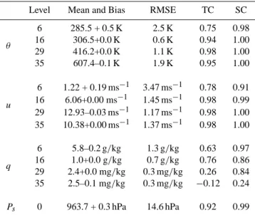
Table 1. Quantitative assessment of model performance in October 1999 with nudging.
Level Mean and Bias RMSE TC SC
θ 6 285.5 + 0.5 K 2.5 K 0.75 0.98 16 306.5+0.0 K 0.6 K 0.94 1.00 29 416.2+0.0 K 1.1 K 0.98 1.00 35 607.4–0.1 K 1.9 K 0.95 1.00 u 6 1.22 + 0.19 ms−1 3.47 ms−1 0.78 0.91 16 6.06+0.00 ms−1 1.45 ms−1 0.98 0.99 29 12.93–0.03 ms−1 1.17 ms−1 0.98 1.00 35 10.38+0.00 ms−1 1.37 ms−1 0.98 1.00 q 6 5.8–0.2 g/kg 1.3 g/kg 0.63 0.97 16 1.0+0.0 g/kg 0.7 g/kg 0.76 0.86 29 2.4+0.0 mg/kg 0.3 mg/kg 0.26 0.84 35 2.5–0.1 mg/kg 0.3 mg/kg −0.12 0.24 Ps 0 963.7 + 0.3 hPa 14.6 hPa 0.92 0.99
Table 2. Quantitative assessment of model performance in October 1999 without nudging.
Level Mean and Bias RMSE TC SC
θ 6 285.0 + 0.1 K 4.5 K 0.26 0.95 16 305.3–1.2 K 5.3 K 0.20 0.94 29 420.1+3.4 K 9.9 K 0.23 0.95 35 608.9+2.2 K 11.0 K 0.26 0.91 u 6 0.75–0.21 ms−1 7.82 ms−1 0.14 0.54 16 6.01–0.07 ms−1 9.49 ms−1 0.19 0.62 29 12.32–0.46 ms−1 8.89 ms−1 0.28 0.81 35 10.12–0.21 ms−1 9.53 ms−1 0.35 0.88 q 6 5.7–0.3 g/kg 1.8 g/kg 0.21 0.94 16 0.9–0.1 g/kg 1.1 g/kg 0.19 0.63 29 2.5+0.1 mg/kg 0.4 mg/kg −0.06 0.81 35 2.5–0.1 mg/kg 0.3 mg/kg −0.14 0.28 Ps 0 964.8 + 1.4 hPa 17.6 hPa 0.17 0.98 3.1.1 Magnitude of differences
The RMSE represents the magnitude of the difference be-tween the model and the ERA-40 data. The addition of nudg-ing reduces the RMSE in all of the assessments made, as shown in Tables 1 and 2, giving evidence that nudging pro-duces better agreement with the ERA-40 data. Figure 2 plots the percentage RMSE of θ between the model with nudging and the ERA-40 data as a function of UM hybrid height level for the three assessment periods. This shows that the RMSE varies little over the height range nudged and over time.
Region of Full Nudging 0 2 8 18 30 46 A p p ro x H e ig h t [ k m ]
Fig. 2. RMSE in θ between the model, with nudging, and the ERA-40 data as a function of UM hybrid height level for the three periods assessed.
The rapid increase in the percentage RMSE towards the top of the model, above the region where nudging is applied, reflects the different treatment of the upper stratosphere be-tween the UM and ECMWF models.
The increase in the RMSE towards the bottom of the model has two components. The increase below level 13 (∼3.5 km) is produced by the fading out of nudging. The increase below level 6 (∼700 m) is caused by different factors. This is partly a result of errors in the vertical interpo-lation used, but is mainly produced by differences over land and ice in the winter.
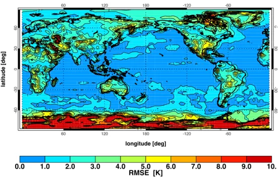
This can more clearly be seen in Fig. 3, which plots the ab-solute RMSE in θ for the UM hybrid height level closest to the surface (20 m above the surface) in July. The largest val-ues occur over Antarctica. In January the RMSE is smaller in Antarctica but larger in the Arctic. These differences proba-bly reflect differences in the heat transfer between the surface and the atmosphere between the UM and ECMWF models. Smaller increases in RMSE can be observed in mountainous regions, such as the Himalayas and the Andes. The low val-ues of RMSE over the Oceans close to the surface, as shown in this figure, demonstrate the benefit of prescribing observed climatological sea surface temperatures.
The RMSE of u shows a similar decrease when nudging is added to the model. The RMSE of q is reduced by nudg-ing, but not so markedly as the RMSE of u or θ . This is to be expected as, though nudging synchronises the large scale dynamics in the model to those in the ERA-40 data, the model physics that determines q is still different. In ad-dition a small amount of noise may still be present in the data nudged to. The representation of q in the stratosphere also suffers from unrealistic initial conditions and, as water content varies slowly here, it is unaffected by nudging in this integration. The RMSE of Ps shows a small decrease with
the addition of nudging, but as the RMSE is dominated by differences in the orography between the ERA-40 data and the model it is little affected by nudging.
0.0 1.0 2.0 3.0 4.0 5.0 6.0 7.0 8.0 9.0 10. RMSE [K] longitude [deg] la ti tu d e [d e g ]
Fig. 3. RMSE in θ between the model, with nudging, and the ERA-40 data for the lowest UM hybrid height level in July 2000.
In general the RMSE in all variables arise from a combi-nation of systematic differences and from incorrectly repro-ducing the temporal variation of the system. These factors are investigated separately by looking at the biases and cor-relations between the model and the ERA-40 data.
3.1.2 Biases in the model
The biases reflect any systematic differences between the model and the ERA-40 data. They are calculated as monthly mean differences between the ERA-40 data and the model, averaged over each model level.
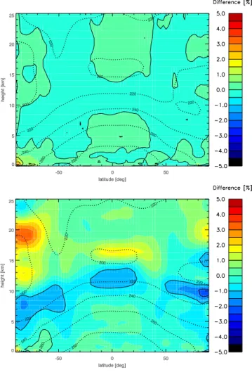
The most notable biases without nudging in the model are those in θ , which are mostly removed by the addition of nudging (Fig. 4). Nudging removes the biases in the up-per troposphere and lower stratosphere, corresponding to the smaller biases observed on the three upper levels in Tables 1 and 2. The removal of these biases is crucial to the modelling of phenomena such as polar stratospheric cloud (PSC) forma-tion and dehydraforma-tion of air passing through the tropopause.
The small bias in level 6 (∼700 m) of the nudged model, located over Antarctica, is attributed to increased cloudiness produced by nudging. The mechanism producing this extra cloudiness is not fully understood. The smaller RMSE with nudging indicates that the addition of nudging still provides a better description of the ERA-40 data. The addition of nudg-ing also reduces biases in u, Ps and, to a lesser degree, q
(Tables 1 and 2).
3.1.3 Representing variability
As well as systematic differences there are differences in the variation of the observables over space and time. The ability of the model to produce the same variation as the ERA-40 data is assessed by the TC and the SC. A comparison between Tables 1 and 2 shows that the addition of nudging increases the correlation between the model and the analyses, with the increase in TC being larger.
Figure 5 shows the TC between the model and the ERA-40 data for u, with and without the addition of nudging, as a function of UM hybrid height level. The TC varies smoothly with height both with and without nudging. The addition of nudging greatly increases the correlation, though TC de-creases below where nudging is cut-off and declines again near the surface where there are errors in the vertical inter-polation of the ERA-40 data. Without nudging the model and the ERA-40 data are very poorly correlated in the tropo-sphere. In the stratosphere the unadjusted model is slightly better at reproducing the variability than in the troposphere.
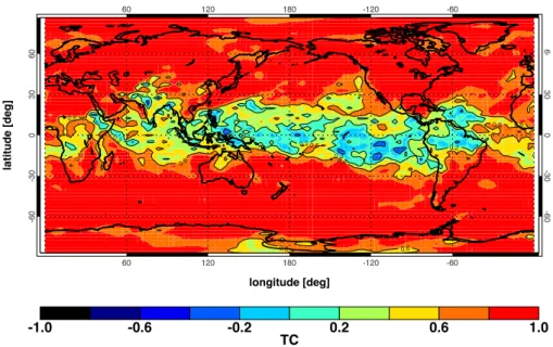
The performance of the model also varies spatially, see for example the TC for θ on UM hybrid height level 6 (∼700 m) (Fig. 6). The TC is high in the extra-tropics, and lower in the tropics, in agreement with Jeuken et al. (1996). The lower TC in this region is not a large problem as the scale of variability is small, as can be seen by the low values of RMSE in this region in Fig. 3.
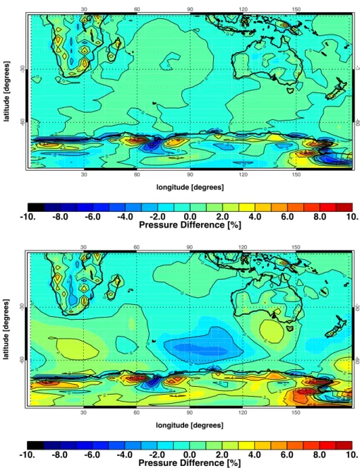
A further illustration of the success of the nudged model in reproducing the variation is given in Fig. 7. The large differ-ences in Ps, a variable that is not adjusted, over the Southern
Fig. 4. Zonal mean bias in θ between the model and the ERA-40 data for October 1999. The top plot is with nudging and the bottom without. Isotherms from ERA-40 are included for reference.
0 2 8 18 30 46 A p p ro x H e ig h t [ k m ]
Fig. 5. TC for u between the model and the ERA-40 data as a function of UM hybrid height level, with and without nudging, in October 1999. The maximum possible value that TC can take, 1, is shown for reference.
Table 3. Statistical Assessments for ω with (w) and without (w/o) nudging.
Level RMSE ( Pa s
−1) TC SC
w w/o w w/o w w/o
925 hPa 0.10 0.11 0.38 0.05 0.40 0.10 500 hPa 0.11 0.17 0.67 0.06 0.70 0.12 50 hPa 0.007 0.009 0.56 0.07 0.67 0.26 10 hPa 0.003 0.003 0.52 0.07 0.53 0.19
Table 4. Precipitation in October 1999 with and without nudging. Mean and Bias RMSE TC SC with nudging 2.44–0.14 mm 5.4 mm 0.56 0.59 without nudging 2.45–0.14 mm 7.2 mm 0.26 0.11
Ocean disappear with the addition of nudging. This is a re-sult of the synoptic scale systems being nudged into the same phase as in the ERA-40 data. The differences in orography can also be seen, especially on the edge of Antarctica. These are responsible for the high RMSE for Ps in the model, as
seen in Tables 1 and 2 .
The differences in the SC with and without nudging are not as dramatic as those in the TC. This is as a result of the unadjusted model reproducing the spatial variation of quan-tities such as temperature and pressure reasonably well on a global scale. For a variable, such as u, in which the spatial variation is not reproduced so well in the unadjusted model, the addition of nudging produces significant increases in the correlation.
3.2 Comparison of derived quantities
In addition to the variables assessed in Sect. 3.1 two other quantities are examined, precipitation and the vertical wind (defined here as ω≡dPdt). The precipitation is derived dif-ferently in both models, so differences are expected due to different treatment of model physics. The vertical wind is a derived quantity in the ECMWF model, but in the UM it is a prognostic quantity, which could result in further differ-ences. In addition the ERA-40 data contains some significant biases, most notably an excess of precipitation over tropical oceans (Uppala et al., 2005). In spite of these difficulties these variables are studied as they can be used to confirm that the model is producing large scale atmospheric motions more like those in the ERA-40 data.
The vertical wind was studied by comparing ω on the ECMWF fixed pressure levels. This is done by calculating RMSE, TC and SC on pressure levels that approximate to
-1.0 -0.6 -0.2 0.2 0.6 1.0 TC longitude [deg] la ti tu d e [d e g ]
Fig. 6. TC for θ between the model, with nudging, and the ERA-40 data for UM hybrid height level 6 (∼700 m) in October 1999.
the UM hybrid height levels used in Sect. 3.1, which are dis-played in Table 3.
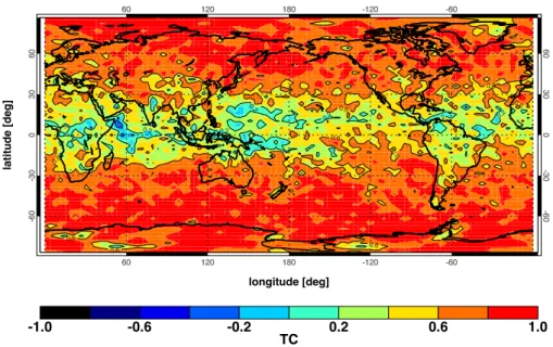
The addition of nudging makes the vertical winds more closely resemble those in ERA-40 data, but there are still large differences, which are not unexpected considering the differences between the UM and ECMWF models. Figure 8 shows the TC for ω at a fixed pressure level of 500 hPa. The same pattern observed in Fig. 6 is seen, with good agreement in the extra-tropics.
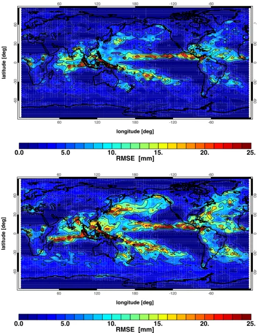
The quantitative assessments used in Sect. 3.1 were ap-plied to the precipitation, as listed in Table 4. The RMSE between the model and then ERA-40 data is shown in Fig. 9. The addition of nudging reduces the differences between the model and the analyses, especially in the extra-tropics. Much of the remaining differences in the tropics can be attributed to errors in the precipitation in the ERA-40 data.
The addition of nudging produces better agreement be-tween the model and the ERA-40 data, especially in the extra-tropics. This reflects the synchronisation of the large scale motion in the model with the ERA-40 data. Much of the remaining differences can be attributed to differences in model physics between the UM and ECMWF models. 3.3 Effects on the model dynamics
The addition of nudging could potentially adversely affect the model dynamics, either by a mismatch with the dynam-ics in the re-analysis or in the addition of spurious “noise”. Any large alteration of the circulation of the model would probably disrupt the vertical winds. The demonstration, in Sect. 3.2, that the vertical wind provides better agreement with the analyses with the addition of nudging increases
con-Table 5. Ratio of tendencies in variables between nudging and all other tendencies.
Level October January July
θ 16 (∼5 km) 0.16 0.16 0.15 29 (∼15 km) 0.36 0.47 0.39 35 (∼20 km) 0.30 0.36 0.43 u 16 (∼5 km) 0.37 0.39 0.43 29 (∼15 km) 0.29 0.40 0.43 35 (∼20 km) 0.30 0.37 0.43
fidence that the model has not been disturbed by the nudging. It is not realistic to make these checks for all aspects of the model, so checks should be made when using variables not described above.
Another check made was to compare the tendency due to nudging to that from all other tendencies for θ and u. This is done by calculating the ratio between the magnitude of these two tendencies, as summarised in Table 5. These values are averaged over all grid-points in each UM hybrid height level and over all time-steps in the month.
There is a degree of variability in time and over the height range, but the tendency due to nudging is never larger than the tendency due to other factors. Figure 10 displays this ratio as a function of UM hybrid height levels for θ for the three assessment periods. The ratio tends to increase with height, showing that the UM has to be forced harder at higher altitudes to agree with the ERA-40 data. This agrees with the conclusions drawn from Fig. 2 that the UM and ECMWF models differ most in the upper stratosphere.
-10. -8.0 -6.0 -4.0 -2.0 0.0 2.0 4.0 6.0 8.0 10. Pressure Difference [%] longitude [degrees] la ti tu d e [d e g re e s ] -10. -8.0 -6.0 -4.0 -2.0 0.0 2.0 4.0 6.0 8.0 10. Pressure Difference [%] longitude [degrees] la ti tu d e [d e g re e s ]
Fig. 7. Difference in surface pressure between the model and the ERA-40 data for a snapshot on 30 October 1999. The top plot shows this with nudging and the bottom without. The region displayed is the eastern half of the Southern Hemisphere.
4 Sensitivity to model parameters
The effect of varying some arbitrary nudging parameters is studied here. This is done by the same assessments used on the default nudging parameters in Sect. 3.1, which will now be denoted the standard assessments. The sensitivity is tested with respect to varying three key parameters: (i) the magnitude of the relaxation parameter used; (ii) the height above which nudging is turned off; and (iii) the ERA-40 data is interpolated from ECMWF fixed pressure levels rather than the original ECMWF hybrid pressure levels. This is de-signed to test our sensitivity to the interpolation in height.
The first sensitivity study was to vary the strength of the relaxation parameter (G) used. Month long runs were made in October 1999 with G reduced by a factor of 10, the weakly
nudged run, and increased by a factor of 10, the strongly nudged run. The results of these runs were analysed using the
standard assessments. The results are tabulated in Table 6 for the weakly nudged run and Table 7 for the strongly nudged run. Comparing to Tables 1 and 2, the weakly nudged run produces better agreement than the run without nudging, but not as good agreement as the standard nudging. The strongly nudged run produces better agreement where the variable is being nudged, but there is no evidence of significant change
-1.0 -0.6 -0.2 0.2 0.6 1.0 TC longitude [deg] la ti tu d e [d e g ]
Fig. 8. TC for ω between the model, with nudging, and the ERA-40 data for fixed pressure level of 500 hPa in October 1999.
Table 6. Quantitative assessment of model performance in October 1999 with weak nudging.
Level Mean and Bias RMSE TC SC
θ 6 284.9–0.2 K 3.3 K 0.54 0.97 16 305.8–0.7 K 2.6 K 0.72 0.99 29 416.7+0.0 K 2.9 K 0.86 0.99 35 607.9–0.7 K 3.5 K 0.85 0.99 u 6 0.97–0.06 ms−1 5.5 ms−1 0.52 0.77 16 6.15+0.08 ms−1 5.0 ms−1 0.76 0.90 29 12.87–0.05 ms−1 3.2 ms−1 0.87 0.97 35 10.45+0.07 ms−1 2.7 ms−1 0.93 0.99 q 6 5.7–0.3 g/kg 1.5 g/kg 0.40 0.96 16 0.9+0.0 g/kg 0.9 g/kg 0.49 0.75 29 2.4+0.0 mg/kg 0.3 mg/kg 0.10 0.85 35 2.5–0.1 mg/kg 0.3 mg/kg −0.09 0.19 Ps 0 964.3 + 0.9 hPa 14.6 hPa 0.71 0.99
in the variables and regions that are not nudged. The ratios of the tendencies due to nudging and all other factors for the strongly and weakly nudged runs are given in Table 8. The table suggests that, for the strongly nudged run, the nudging becomes the dominant tendency.
The evidence indicates that the relaxation parameter cho-sen originally is a reasonable choice, producing significant improvement in the description of the ERA-40 data without predominating over the model’s physical tendencies.
Table 7. Quantitative assessment of model performance in October 1999 with strong nudging.
Level Mean and Bias RMSE TC SC
θ 6 285.8+0.8 K 2.6 K 0.77 0.98 16 306.6+0.0 K 0.2 K 0.99 1.00 29 416.0+0.0 K 0.3 K 1.00 1.00 35 607.6+0.0 K 0.8 K 0.99 1.00 u 6 1.09+0.06 ms−1 3.09 ms−1 0.82 0.93 16 6.05–0.01 ms−1 0.40 ms−1 1.00 1.00 29 12.96+0.01 ms−1 0.46 ms−1 1.00 1.00 35 10.38+0.01 ms−1 0.59 ms−1 1.00 1.00 q 6 5.8–0.3 g/kg 1.2 g/kg 0.66 0.97 16 1.0+0.1 g/kg 0.7 g/kg 0.78 0.88 29 2.4+0.0 mg/kg 0.4 mg/kg 0.30 0.80 35 2.5–0.1 mg/kg 0.3 mg/kg −0.12 0.24 Ps 0 963.9 + 0.4 hPa 15.4 hPa 0.93 0.99
We apply nudging to as great a height possible, only excluding where the quality of the ERA-40 data becomes doubtful. The ECHAM model3 has been run in a configu-ration where the nudging is applied in the troposphere alone and see little difference to the case where nudging is applied into the stratosphere (J¨ockel et al., 2006). We perform a sim-ilar exercise by turning nudging off above model level 31
0.0 5.0 10. 15. 20. 25. RMSE [mm] longitude [deg] la ti tu d e [d e g ] 0.0 5.0 10. 15. 20. 25. RMSE [mm] longitude [deg] la ti tu d e [d e g ]
Fig. 9. RMSE for precipitation between the model and the ERA-40 data in October 1999. The top plot is with and the bottom plot without nudging.
Table 8. Ratio of tendencies in variables between nudging and all other tendencies for the strongly and weakly nudged runs.
Level θ u
strong weak strong weak 16 (∼5 km) 0.61 0.09 0.83 0.15 29 (∼15 km) 0.92 0.14 1.02 0.18 35 (∼20 km) 1.01 0.10 1.11 0.09
(∼19 km), above the tropical tropopause. The standard as-sessments were performed again, producing results very sim-ilar to those in Sect. 3.1 in the lowest three assessed levels, but differ on the highest assessed level, level 35 (∼20 km), from which the results are tabulated in Table 9. There is still considerable improvement with respect to the case with no nudging, but not enough to justify using this lower cut-off.
The ERA-40 data is originally produced on hybrid pres-sure levels but is made available interpolated onto a set of fixed pressure levels. The last study is to take the ERA-40 data on these fixed pressure levels.
0 2 8 18 30 46 Height [k m] 84 Ratio of Forcings
Fig. 10. Ratio of tendency due to nudging to all other tendencies for θ for October 1999 and January and July 2000.
-2.5 -2.0 -1.5 -1.0 -0.5 0.0 0.5 1.0 1.5 2.0 2.5 Difference [%]
Fig. 11. Zonal mean difference in θ on UM hybrid height levels between ERA-40 data on fixed pressure levels and hybrid pressure levels. Isotherms from ERA-40 are included for reference.
A run is made for October 1999 and the standard assess-ments made. If we compare the model output to the ERA-40 data on fixed pressure levels interpolated on to UM hybrid height levels we see results that are similar to those seen in Sect. 3.1. However if we compare the model output to ERA-40 data on the hybrid pressure levels interpolated on to the UM hybrid height levels we see discrepancies. These differ-ences result from the additional interpolation to produce the ERA-40 data on fixed pressure levels. They are insignificant in the troposphere, but produce significant differences around the tropopause and above, in regions where the gradient is steep, such as the tropical tropopause and just below 20 km above Antarctica. The gentler vertical gradients in u and v result in much smaller differences.
The differences produced by this additional interpolation also give an indication of sensitivity to the interpolation of
Table 9. Quantitative assessment for model level 35 (∼20 km) in October 1999 with “tropospheric only” nudging.
Mean and Bias RMSE TC SC
θ 606.0–1.0 K 6.6 K 0.69 0.97
u 9.96–0.41 ms−1 3.63 ms−1 0.88 0.98
q 2.5–0.1 mg/kg 0.3 mg/kg −0.11 0.26
the ERA-40 data onto the UM hybrid height levels. The small size of the differences throughout most of the atmo-sphere indicates that the interpolation is not introducing large errors.
5 Conclusions
We have described a nudged version of the “New Dynamics” Unified Model and demonstrate that it reproduces the ERA-40 data better compared to the model without nudging. This is the first detailed description of the dynamics of a nudged grid-point model and we have noted similar features to those seen in nudged spectral models.
The addition of nudging reduces biases between the model and the ERA-40 data, such as those in θ in the strato-sphere (Fig. 4). The variability of the ERA-40 data is demon-strated to be well reproduced (Fig. 5) with the addition of nudging, even in variables not directly adjusted such as q and ω (Figs. 8 and 9). This reflects that the “weather” is rea-sonably well represented. The strength and height regime of nudging were varied to demonstrate that the parameters cho-sen are reasonable.
Future work will concentrate on the behaviour of trac-ers, with the nudged model being used to evaluate the new UK chemistry and aerosol (UKCA) chemistry climate model (CCM), which is also based on the UM. The removal of bi-ases should aid the modelling of phenomena sensitive to the model dynamics, such as polar stratospheric cloud formation. A reasonable representation of the weather allows episodic data to be used, expanding the available data sets that can be used to evaluate the model.
In conclusion the addition of nudging allows better corre-spondence with global meteorological re-analysis data to be obtained and will provide a powerful tool for studying as-pects of the UM on short time-scales.
Acknowledgements. This work was supported by NCAS. We also acknowledge support through the EU FP6 Integrated Programme, SCOUT-O3.
References
Brill, K., Uccellini, L., Manobianco, J., Kocin, P., and Homan, J.: The use of successive dynamic initialization by nudging to simu-late cyclogenesis during GALE-IOP, 1, Meteorol. Atmos. Phys., 45, 15–40, 1991.
Dean, S. M., Flowerdew, J., Lawrence, B. N., and Eckermann, S. D.: Parameterisation of orographic cloud dynamics in a GCM, Clim. Dynam., 28, 581–597, 2006.
ECMWF: The Description of the ECMWF Re-analysis Global At-mospheric Data Archive, ECMWF, 1996.
Hauglustaine, D., Hourdin, F., Jourdain, L., Filliberti, M., Wal-ters, S., Lamarque, J., and Holland, E.: Interactive chem-istry in the Laboratoire de M´et´eorolgie Dynamique gen-eral circulation model: Description and background tropo-spheric chemistry evaluation, J. Geophys. Res., 109, 4314, doi:10.1029/2003JD003957, 2004.
Jeuken, A., Siegmund, P., Heijboer, L., Feichter, J., and Bengtsson, L.: On the Potential of assimilating meteorological analyses in a global climate model for the purposes of model validation, J. Geophys. Res., 101, 16 939–16 950, 1996.
J¨ockel, P., Tost, H., Pozzer, A., Br¨uhl, C., Buchholz, J., Ganzeveld, L., Hoor, P., Kerkweg, A., Lawrence, M.G., Sander, R., Steil, B., Stiller, G., Tanarhte, M., Taraborrelli, D., van Aardenne, J., and Lelieveld, J.: The atmospheric chemistry general circulation model ECHAM5/MESSy1: consistent simulation of ozone from the surface to the mesosphere, Atmos. Chem. Phys., 6, 5067– 5104, 2006,
http://www.atmos-chem-phys.net/6/5067/2006/.
Lorenc, A., Andrews, P., Ballard, S., Clayton, A., Ingleby, N., Li, D., Payne, T., and Saunders, F.: Design and Testing of the Met Office Variational Data Assimilation Scheme, Technical Report 262, Met Office, 1999.
Pyle, J. A., Braesicke, P., and Zeng, G.: Dynamical variability in the modeling of chemistry-climate interactions, Faraday Discuss., 130, 27–39, 2005.
Rayner, A., Parker, D., Horton, E., Folland, C., Alexander, L., Rowell, D., Kent, E., and Kaplan, A.: Global analyses of sea surface temperature, sea ice, and night marine air temperature since the late nineteenth century, J. Geophys. Res., 108D, 4407, doi:10.1029/2000JD900205, 2003.
Schmidt, G., Ruedy, R., Hansen, J., Aleinov, I., Bell, N., Bauer, M., Bauer, S., Cairns, B., Canuto, V., Cheng, Y., Del Genio, A., Faluvegi, G., Friend, A., Hall, T., Hu, Y., Kelley, M., Kiang, N., Koch, D., Lacis, A., Lerner, J., Lo, K., Miller, R., Nazarenko, L., Oinas, V., Perlwitz, J., Perlwitz, J., Rind, D., Romanou, A., Russell, G., Sato, M., Shindell, D., Stone, P., Sun, S., Tausnev, N., Thresher, D., and Yao, M.-S.: Present day atmospheric simu-lations using GISS ModelE: Comparison to in-situ, satellite and reanalysis data, J. Climate, 19, 153–192, 2006.
Staniforth, A., White, A., Wood, N., Thuburn, J., Zerroukat, M., Cordero, E., and Davies, T.: Joy of U.M. 6.1 – Model Formula-tion, United Kingdom Meteorological Office (UKMO), 2005. Takemura, T., Okamoto, H., Maruyama, Y., Numaguti, A.,
Hig-urashi, A., and Nakajima, T.: Global three dimensional simula-tion of aerosol optical thickness distribusimula-tion of various origins, J. Geophys. Res., 105, 17 853–17 873, 2000.
Uppala, S., Kallberg, P., Simmons, A., Andrae, U., da Costa Bech-told, V., Fiorino, M., Gibson, J., Haseler, J., Hernandez, A., Kelly, G., Li, X., Onogi, K., Saarinen, S., Sokka, N., Allan, R., Andersson, E., Arpe, K., Balmaseda, M., Beljaars, A., van de Berg, L., Bidlot, J., Bormann, N., Caires, S., Chevallier, F., De-thof, A., Dragosavac, M., Fisher, M., Fuentes, M., Hagemann, S., Holm, E., Hoskins, B., Isaksen, L., Janssen, P., Jenne, R., Mc-Nally, A., Mahfouf, J.-F., Morcrette, J.-J., Rayner, N., Saunders, R., Simon, P., Sterl, A., Trenberth, K., Untch, A., Vasiljevic, D., Viterbo, P., and Woollen, J.: The ERA-40 re-analysis, Q. J. Roy. Meteor. Soc., 131, 2961–3012, 2005.
van Aalst, M., van den Broeck, M., Bregman, A., Br¨uhl, C., Steil, B., Toon, G., Garcelon, S., Hansford, G., Jones, R., Gardiner, T., Roelofs, G., Lelieveld, J., and Crutzen, P.: Trace Gas Trans-port in the 1999/2000 Arctic winter: comparison of nudged GCM runs with observations, Atmos. Chem. Phys., 4, 81–93, 2004, http://www.atmos-chem-phys.net/4/81/2004/.