Publisher’s version / Version de l'éditeur:
Vous avez des questions? Nous pouvons vous aider. Pour communiquer directement avec un auteur, consultez la première page de la revue dans laquelle son article a été publié afin de trouver ses coordonnées. Si vous n’arrivez pas à les repérer, communiquez avec nous à [email protected].
Questions? Contact the NRC Publications Archive team at
[email protected]. If you wish to email the authors directly, please see the first page of the publication for their contact information.
https://publications-cnrc.canada.ca/fra/droits
L’accès à ce site Web et l’utilisation de son contenu sont assujettis aux conditions présentées dans le site LISEZ CES CONDITIONS ATTENTIVEMENT AVANT D’UTILISER CE SITE WEB.
Proceedings of the 7th Workshop on NLP for Similar Languages, Varieties and
Dialects, pp. 273-282, 2020-12-13
READ THESE TERMS AND CONDITIONS CAREFULLY BEFORE USING THIS WEBSITE.
https://nrc-publications.canada.ca/eng/copyright
NRC Publications Archive Record / Notice des Archives des publications du CNRC :
https://nrc-publications.canada.ca/eng/view/object/?id=c82dee32-2231-490d-b134-50cb2490601d https://publications-cnrc.canada.ca/fra/voir/objet/?id=c82dee32-2231-490d-b134-50cb2490601d
NRC Publications Archive
Archives des publications du CNRC
This publication could be one of several versions: author’s original, accepted manuscript or the publisher’s version. / La version de cette publication peut être l’une des suivantes : la version prépublication de l’auteur, la version acceptée du manuscrit ou la version de l’éditeur.
Access and use of this website and the material on it are subject to the Terms and Conditions set forth at
Challenges in neural language identification: NRC at VarDial 2020
Proceedings of the 7th VarDial Workshop on NLP for Similar Languages, Varieties and Dialects, pages 273–282 Barcelona, Spain (Online), December 13, 2020
273
Challenges in Neural Language Identification: NRC at VarDial 2020
Gabriel Bernier-Colborne, Cyril Goutte National Research Council Canada
{Gabriel.Bernier-Colborne, Cyril.Goutte}@nrc-cnrc.gc.ca
Abstract
We describe the systems developed by the National Research Council Canada for the Uralic lan-guage identification shared task at the 2020 VarDial evaluation campaign. Although our official results were well below the baseline, we show in this paper that this was not due to the neural ap-proach to language identification in general, but to a flaw in the function we used to sample data for training and evaluation purposes. Preliminary experiments conducted after the evaluation period suggest that our neural approach to language identification can achieve state-of-the-art results on this task, although further experimentation is required.
1 Introduction
The goal of the Uralic language identification (ULI) shared task at VarDial 2020 (G˘aman et al., 2020) was to identify and discriminate 29 Uralic language varieties. This involves distinguishing the relevant languages from a large set of non-relevant languages and discriminating between these languages.
To solve this task, we used an approach similar to the one we developed for the cuneiform language identification shared task at VarDial 2019 (Bernier-Colborne et al., 2019). This approach was ranked first in that competition, which was one of the first times a language identification shared task was won by a neural network (Zampieri et al., 2019). It is a deep learning approach based on character embeddings and a transformer network (Vaswani et al., 2017) trained in a similar fashion to BERT (Devlin et al., 2019).
On this year’s ULI shared task, we did not have the same level of success using this neural approach to language identification, as our accuracy scores on the held-out test set were significantly lower than the baseline scores.
In this paper, we explore the challenges presented by the ULI task and explain the reasons for the low accuracy scores achieved by our model in the official evaluation. We then show that neural language identification can produce much better results if trained and tuned correctly.
2 Task Definition and Data
The goal of this language identification task is simply to identify the language of a given text, which is typically a single sentence. If more than one language is used in the text (e.g. code switching), the main language must be identified. Since there are both relevant and non-relevant languages in the test set, the task involves not only discriminating amongst the relevant languages, but also distinguishing them from the non-relevant languages. The shared task was closed, so no data could be used except for the training set provided.
The task was subdivided into three tracks. The training and test data is the same for all three tracks, the difference being the way in which evaluation metrics are computed. For tracks 1 and 2, only test cases where either the predicted or true label is a relevant language are evaluated, using macro-averaged and micro-averaged F1 score respectively. For track 3, all test cases are evaluated, using the macro-averaged F1 score.
This work is licensed under a Creative Commons Attribution 4.0 International Licence. Licence details: http:// creativecommons.org/licenses/by/4.0/.
274
The 29 relevant languages for this task are part of the Uralic group of languages, which are spoken mainly in northern Eurasia. Some of these languages are very under-resourced, and some are already extinct, e.g. Kemi Saami, which was represented in this task.
Also included in the test set are 149 other languages considered non-relevant. These include the three largest Uralic languages (i.e. Estonian, Finnish, and Hungarian), as well as a wide variety of other languages. In total, 178 languages or language varieties were represented in this task, the highest number covered so far in a language identification shared task.
The training set provided contains 646,043 examples for the relevant languages and 63,772,445 exam-ples for the non-relevant ones. Thus, there is much less data for the relevant languages, on average. Both the relevant and non-relevant portions of the training set are (highly) unbalanced. The class frequencies in the relevant training data range from 19 (Kemi Saami) to 214,225 (Northern Saami). The non-relevant portion of the dataset contains anywhere from 10,000 to 3,000,000 examples per class (i.e. language).
The training set was compiled from 2 different sources: data for the relevant languages comes from the Wanca 2016 corpus (Jauhiainen et al., 2019a), whereas the non-relevant data was extracted from the Leipzig corpus (Goldhahn et al., 2012). The relevant data in the held-out test set comes from the Wanca 2017 dataset. For more information on the dataset, the task, and the baseline scores, refer to Jauhiainen et al. (2020).
Regarding the length of the texts, for relevant languages, 86% of the texts contain 128 characters or less, and only 1.2% are longer than 256 characters. For non-relevant languages, 70% of texts contain 128 characters or less, and 0.02% are longer than 256 characters.
Note that there are no duplicates in the relevant training data. In the non-relevant training data, less than 0.5% of examples appear more than once (whether in the same language or different languages). 2.1 Challenges
The ULI shared task presented many challenges. Some of these challenges are inherent to language identification in general. For instance, some of the target languages are very closely related, such as Ingrian, Ludian, and Karelian (Jauhiainen et al., 2020). This can make it hard to distinguish between such languages. Furthermore, some languages are spoken and written much more frequently than others, such that there are often large class imbalances in datasets for language identification. In the case of the ULI task, some language varieties have so little data available that it was announced at the outset that some relevant languages would not be present in the held-out test set. In general, detecting very rare languages is challenging, especially if they are closely related to other languages present in the training data.
The ULI shared task presented its own specific challenges. There are not only large class imbalances within the relevant and non-relevant groups, but also a large discrepancy between these two groups, as there is about 100 times more training data for the non-relevant languages, meaning that their frequency is about 20 times greater on average than the relevant languages (as there are about 5 times more non-relevant than non-relevant languages). These large and complex class imbalances make this a tricky task to learn.
The training set is also quite large, so simply processing all that data may incur a high computational cost. Using a neural model such as a large transformer network, simply encoding all the texts may take a long time. So finding a way to efficiently train and tune a model on such a large dataset may be challenging.
Another potential challenge posed by the ULI task is the presence of noise (i.e. incorrectly labeled sentences) in the training data, as the corpora were produced in part using automatic web crawling and language identification methods.
Finally, a challenge that turned out to have a huge impact on our results is the fact that the organizers decided not to provide a dedicated development set; just a training set. This is a legitimate design decision for such a competition, which entails that participants must create their own development set from the training data. The adequacy of this development set is very important to estimate the accuracy that the model will achieve on the held-out test data, and select the best models.
275
3 A Neural Approach to Language Identification
The neural approach we used for this task is similar to the one we developed for the cuneiform language identification shared task at VarDial 2019. The model is a deep neural network which takes sequences of characters as input. The model is trained in two stages: (partially) self-supervised pre-training, and supervised fine-tuning. Typically, when training this type of model, the pre-training phase would exploit large amounts of unlabeled text data, then the subsequent fine-tuning phase would exploit a much smaller amount of labeled data. Since the ULI shared task was a closed one, we used the same training set for both pre-training and fine-tuning.
The network is composed of a stack of bidirectional transformer modules (Vaswani et al., 2017) which encode the input sequence. The output of this encoder is fed to one or more output layers, which depend on the tasks used for pre-training and fine-tuning.
First, we pre-train the model using 2 pre-training tasks: masked language modeling (MLM) and sen-tence pair classification (SPC). The MLM task is exactly as described by Devlin et al. (2019). The objective is to predict tokens (in this case, characters) chosen at random based on all the other tokens in the text. This produces a model that can predict characters in context for any of the languages rep-resented in the training data (with varying degrees of accuracy), and must therefore have learned the specific patterns of each language (or at least some of them).
As for the SPC pre-training task, it is similar to the next sentence prediction task proposed by Devlin et al. (2019), but we adapted it for language identification. Instead of predicting whether two sequences follow each other in the training corpus, we predict whether two sequences are in the same language. This introduces a supervised signal into the pre-training task (whereas MLM is self-supervised), as we use the labels in the training data in order to label pairs of texts as belonging to the same language or not. Learning to predict whether two texts belong to the same language should be helpful to predict the language used in a specific text, when we fine-tune the model on this task later on.
Thus, the pre-training phase uses two different output layers, one for MLM and one for SPC. The first is a simple softmax over the vocabulary, which is composed of characters in this case. The input of this layer is the encoding of a character in the sequence that has been masked beforehand: before feeding the sequence to the encoder, we pick some characters at random and replace them with a special masking token. Based on the encoding of a masked token (which encodes information about the other tokens in the sequence), the softmax layer is used to predict the most likely character. For more details on the implementation of masked language modeling, refer to Devlin et al. (2019).
The second output layer is a binary classifier which applies average pooling over the final hidden states of the encoder for each of the two input texts (separately), then computes the dot product of the two pooled encodings, then predicts whether the two input texts belong to the same language based on this similarity function. Texts whose pooled encodings are similar will therefore be predicted to belong to the same language. Note that this bi-encoding approach to SPC has a lower computational cost than the cross-encoding approach we used for cuneiform language identification at VarDial 2019, where both sequences are concatenated and encoded together. The cost remains quadratic with respect to the length of the sequence, but the sequence is half as long, and we encode two sequences instead of one.
Once the model is pre-trained, we fine-tune it on the target task, which is to predict the language of each text, using the labeled training data. For this, we use the pre-trained encoder, and add a new output layer for language identification, which is simply a softmax over the 178 languages.
The loss function used to learn all tasks is cross-entropy, which is commonly used for multi-class classification problems, averaged across examples in a batch. We did not assign class-specific cost weights, but we did experiment with oversampling of the training data during fine-tuning, which plays a similar role in alleviating class imbalances (see related work in Sec. 7). In cases where we used multiple tasks at once for training, losses were summed.
The vocabulary (or alphabet) of symbols for which we learn embeddings is composed of every charac-ter in the training set whose frequency is greacharac-ter than some threshold, plus a few reserved symbols (e.g. unknown characters and padding). In the experiments we carried out on our own train/dev/test split, we computed the vocab on the training portion only. Using a minimum frequency of 2, this produced
276
a vocab of about 15K characters. Input characters that are not part of the vocabulary are mapped to a special symbol for unknown characters.
For efficiency, we used a small architecture containing only 8 transformer layers, rather than the 12 layers of the “base” architecture proposed by Devlin et al. (2019). Our other hyperparameter settings for pre-training largely follow their recommendations:
• Nb transformer layers: 8 • Nb attention heads: 12 • Hidden layer size: 768 • Feed forward/filter size: 3072 • Hidden activation: gelu • Dropout probability: 0.1
• Optimizer: Adam (with β1= β2= 0.9) • Learning rate: 1e-4
• Warmup steps for pre-training: 10K • Maximum input length: 128
For fine-tuning, we experimented with different values for the batch size and learning rate. We also tested a longer maximum input length of 256. In this case, the position embeddings that were not used during pre-training, and are therefore still randomly initialized, are learned on the fly during fine-tuning. Note that no pre-processing was applied to the input text (e.g. word or sub-word tokenization, charac-ter normalization, etc.).
We used a single GPU (Nvidia K80 or V100, depending on the experiment) with 12 GB of memory for both pre-training and fine-tuning. Note that simply producing the predictions of the model on the held-out test set, containing over 1.5 million examples, took about 8 hours on a V100 (with a batch size of 64 and a maximum sequence length of 256).
Our code, which exploits the Transformers library by HuggingFace (Wolf et al., 2020), is available is at https://www.github.com/gbcolborne/vardial2020.
4 Methodology
To produce our systems for the ULI task, we experimented with various training tasks and hyperparame-ter settings, and selected the models that seemed to perform best. Before we could do this, we first had to create a dev set, as none was provided for this task. A dev set was necessary to tune the hyperparameters of the model and to estimate the accuracy we could expect to achieve on the held-out test set. To get an unbiased estimate of held-out accuracy, we created two dev sets, one used to tune hyperparameters, and the other to evaluate the fully tuned model. We will call the former ‘dev’ and the latter ‘dev-test’ when needed to distinguish the two. In the following sections, we explain how we split the training data to obtain these dev sets, then provide an overview of our model selection experiments.
4.1 Splitting the Data
Before sampling a dev set from the ULI training data, we have to consider the fact that there is 20 times more data for the non-relevant languages than the relevant ones, on average, and that both the relevant and non-relevant data are unbalanced. If we sampled examples at random, without considering the relative class frequencies, we would have to sample a very large number of examples in order to get a decent coverage of all the languages in the training data.
277
• They should be large enough to estimate the evaluation metrics accurately, yet not so large that running the evaluation would be prohibitively expensive in terms of computation time. Something on the order of 10,000-100,000 examples seemed reasonable.
• They should cover most of the relevant languages, but not necessarily all of them, as we knew from the outset that some relevant languages would not appear in the held-out test set. We decided to ensure that a few of the rarest languages would be absent from our dev sets.
We also thought it might be helpful to sample the three non-relevant Uralic languages more frequently than the other non-relevant languages. The motivation was that these three languages would likely be the hardest to distinguish from the 29 relevant languages.
To sample our dev sets, we computed the relative class frequencies separately for these three groups: relevant, non-relevant Uralic, and non-relevant non-Uralic. Then, we sampled from each of these three groups independently, by setting the sampling probability of each language in a group to its relative frequency. We sampled two dev sets containing 12,000 examples each. In each of them, three of the relevant languages were absent.
After the official evaluation, we figured out that there was a major flaw in the way we sampled data to create the dev sets. By analyzing the class distribution of these dev sets, we observed that the three non-relevant Uralic languages were being sampled much more often than either the relevant languages or the 146 other non-relevant languages. This was because we sampled uniformly from the 3 groups, ignoring the fact that there were far fewer languages in the non-relevant Uralic group. This made our dev sets bad estimators of held-out test accuracy. This would affect not only model selection, but also the training itself, as we used a similar function to resample the training data. More details on the effect of this mistake are provided in Sec. 5.
4.2 Model Selection
While developing our system, we empirically investigated questions such as:
• Does doing SPC along with MLM during pre-training improve classification accuracy after fine-tuning?
• Does doing MLM on the labeled training data along with language identification during fine-tuning improve classification accuracy?
• Does doing MLM on the unlabeled dev or test data during fine-tuning (to adapt the encoder to the unlabeled data) improve classification accuracy?
• What are the optimal settings of those hyperparameters of the BERT method that are known to have a significant impact on accuracy (e.g. batch size, learning rate, number of training steps, etc.). • Does increasing the maximum input length to 256 during fine-tuning improve classification
accu-racy?
• Does damping the relative class frequencies used for sampling improve accuracy?
We will not go into the details of these experiments here. Because of the flaw in the sampling function we used to sample our dev sets, the results of these experiments are of little interest.
We ended up submitting the predictions of three different systems for each of the three tracks. For each track, we submitted the predictions of:
• A model trained on all the training data, using the optimal settings for a given track according to our model selection experiments. This model was pre-trained with both MLM and SPC, and fine-tuned with both MLM and language identification.
• Same as the previous model, but during fine-tuning, we ran MLM on the unlabeled, held-out test set alongside MLM and language identification on the labeled training data.
278
• An ensemble of 6 models, i.e. the two previous models for each of the three tracks. We used plurality voting. To break ties, we favoured the model tuned for a given track (with adaptation to the unlabeled test data).
5 Official Results
We were the only team who participated in the ULI task (perhaps because of some of the challenges we have outlined in this paper), therefore we can only compare our results to the baseline scores computed by the organizers. The baseline scores were computed using the HeLI method (Jauhiainen et al., 2017).
System Track 1 (macro F1, rel.) Track 2 (micro F1, rel.) Track 3 (macro F1, all) Best run 0.300 0.260 0.675 Baseline 0.802 0.973 0.926
Table 1: Score of our best run on the held-out test set. For tracks 1 and 2, only the test cases where either the predicted or true label is a relevant language are evaluated. For track 3, all test cases are evaluated. Also shown are the scores of the baseline system, i.e. HeLI.
Our best score on each of the three tracks is shown Table 1 along with the baselines. It is obvious from these results that our models performed very poorly on the held-out test set. Our scores were not only much lower than the baseline, but also much lower than the scores we had estimated on our own dev sets. Looking at our precision and recall scores on track 2, we observed that recall was relatively high (0.895), but precision was very low (0.085), indicating that our model was badly over-detecting relevant languages.
Faced with these results, we set about figuring out what went wrong. Was this neural approach simply inadequate for this language identification task or was there some flaw in the way we trained and selected our models? The fact that our dev sets had significantly overestimated our held-out accuracy suggested that the latter explanation was plausible.
6 Post-evaluation Experiments
To confirm our suspicion that our dev sets were bad estimators of held-out test accuracy, we evaluated the baseline method, i.e. HeLI, on our split of the training data. We used a different implementation of HeLI than the organizers, but our settings were similar to those reported by Jauhiainen et al. (2020). We used the implementation that is publicly available at https://github.com/tosaja/HeLI, and modified the settings in the HeLI.java class as follows: we only used lower-case features, all feature count thresholds were increased from the default 1000 to 300,000, the maximum n-gram length was set to 6, and the penalty was set to 7.
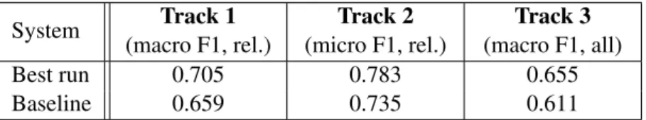
System Track 1 (macro F1, rel.) Track 2 (micro F1, rel.) Track 3 (macro F1, all) Best run 0.705 0.783 0.655 Baseline 0.659 0.735 0.611
Table 2: Scores on our dev set before the sampling flaw was corrected.
The baseline scores we obtained on our dev set are shown in Table 2, along with the best dev score we observed when training the neural models. These results indicated that the baseline system’s scores were similar to those of our neural network, and much lower than the scores achieved by the baseline system on the held-out test set. This corroborated our suspicion that there was a flaw in the function we used to sample the dev sets, which made them bad estimators of held-out test accuracy.
Since we used a similar function to sample the training data, optimization of the parameters of the neural network was also affected. The combination of these two factors explains why our system’s scores were so much lower than the baseline scores in the official evaluation.
279
Equipped with this knowledge, we set about re-evaluating our neural approach to see if it could achieve a similar level of accuracy as the baseline method on a more representative dev set. Due to time con-straints, we were not able to conduct a thorough assessment of this question, but we report the results of our preliminary experiments below.
6.1 Fixing the Sampling Function
We produced new dev sets using a corrected sampling procedure. First, we compute relative frequen-cies of relevant and non-relevant languages separately. Then we compute sampling probabilities of the languages in the two groups using the following function:
Pi(x) =
fi(x)α P
x0fi(x0)α
where Pi(x) is the sampling probability of language x in group i (relevant or non-relevant), fi(x) returns the relative frequency of x within its group, α is a damping factor between 0 and 1 (with 0 producing a uniform distribution), and the denominator of the term on the right normalizes over all the languages in the group.
To get a distribution over all languages, we combine the distributions for relevant and non-relevant languages. The probability of language x is given by computing the score s(x) as follows and renormal-izing: s(x) = ( γPrelevant(x), if x is relevant Pnon-relevant(x), otherwise P (x) = Ps(x) x0s(x0)
Here, γ is the relative weight of relevant examples with respect to non-relevant ones, e.g. γ = 2 means we would sample relevant examples approximately twice as often as non-relevant ones. So this is basi-cally interpolating between a distribution where only non-relevant languages have non-zero probability (with γ = 0) and a distribution where the opposite is true (as γ → ∞).
Using this probability distribution, with α = 1 and γ = 1, we sampled a dev set containing 20,000 examples and a dev-test set containing 100,000 examples.
6.2 Experiments
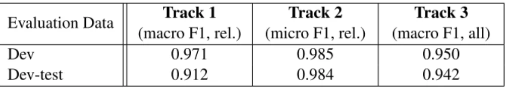
We first tested the baseline system on our new split of the training data. Scores are shown in Table 3. These scores are similar to the baseline scores computed on the held-out test set by the organizers. This indicated that our new dev sets were good (or at least better) estimators of held-out test accuracy.
Evaluation Data Track 1 (macro F1, rel.) Track 2 (micro F1, rel.) Track 3 (macro F1, all) Dev 0.971 0.985 0.950 Dev-test 0.912 0.984 0.942
Table 3: Scores of the baseline system (i.e. HeLI) on our corrected dev sets.
We then trained our neural model using the corrected sampling function to sample training examples. After pre-training the model on our training set for about 700,000 steps, we did a small fine-tuning grid search in order to begin exploring the following questions:
• Does damping the sampling probabilities for training (with α < 1) help?
• Does sampling relevant examples more often than non-relevant ones during training (with γ > 1) help?
280
• Does doing MLM along with language identification help?
• Should we fine-tune the whole model or freeze the weights of the encoder? Accordingly, we tested every combination of the following settings:
• α = { 1, 0.75 } • γ = { 1, 2 }
• Tasks = { SPC only (frozen encoder), SPC only (full fine-tuning), MLM+SPC (full fine-tuning) } As for the other hyperparameters, we used the following settings, which had worked well in our previous experiments: maximum input length = 128, learning rate = 3e-5, batch size = 32. When the encoder was frozen, batch size was increased to 128. We fine-tuned the 12 models for as long as possible given the time left before the deadline to submit this paper. We used early stopping for model selection, optimizing for track 3 when γ = 1 and for track 1 when γ = 2; we did not optimize any models for track 2.
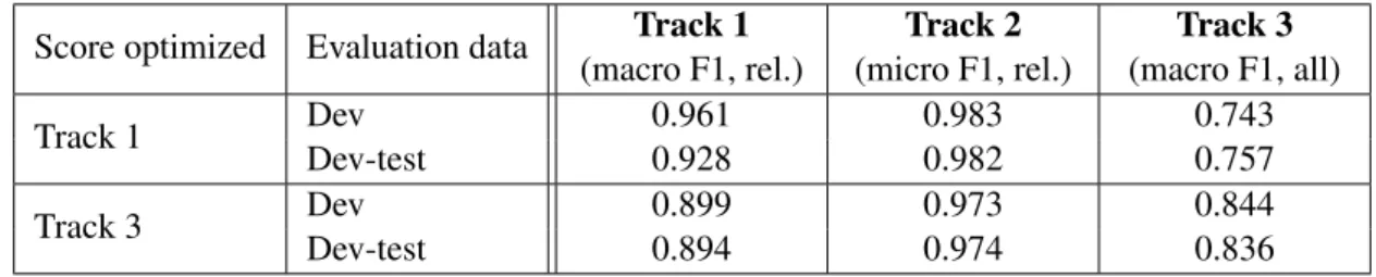
Score optimized Evaluation data Track 1 (macro F1, rel.) Track 2 (micro F1, rel.) Track 3 (macro F1, all) Track 1 Dev 0.961 0.983 0.743 Dev-test 0.928 0.982 0.757 Track 3 Dev 0.899 0.973 0.844 Dev-test 0.894 0.974 0.836
Table 4: Scores of the neural model on our corrected dev sets. Score on ‘dev’ is the best dev score achieved for a given track during training. Score on ‘dev-test’ is the score of the corresponding (early-stopped) model on our ‘dev-test’ set.
The best dev scores and the scores of the corresponding (early-stopped) models on the dev-test set are shown in Table 4. Comparing these results to the baseline scores in Table 3, we can see that the neural model achieved a higher score on the dev-test set for track 1 (0.928 vs. 0.912), a slightly lower score for track 2 (0.982 vs. 0.984), and a significantly lower score for track 3 (0.836 vs. 0.942). Below, we briefly investigate why our track 3 score is still well below that of the baseline method.
The hyperparameter settings that were optimal for track 1 according to the grid search were: SPC only (full fine-tuning), α = 0.75, γ = 2. The best dev score was achieved after 510,000 steps. As for track 3, the optimal settings were: SPC only (with frozen encoder), α = 0.75, γ = 1. The best dev score was achieved after 715,000 steps.
These results suggest that damping the relative class frequencies when computing the sampling prob-abilities for training was effective, and that sampling relevant examples more often was helpful for track 1, where we only evaluate test cases where either the gold or predicted label is a relevant language. It also appears that doing MLM alongside SPC during fine-tuning was not helpful, although more exten-sive experiments would be required to confirm this. Finally, freezing the encoder was helpful for track 3, perhaps because in this case we increased the batch size from 32 to 128, which allowed the model to observe more training data.
Given the time available, we were only able to fine-tune for about 750,000 steps, and the best track 3 dev score was achieved near the end of this, after step 715,000. Given that the batch size was 128 and γ = 1, the model was able to observe about 45M non-relevant examples in total, which is about 3/4 of the available training data for non-relevant languages. As it is usually recommended to do 3 or 4 epochs during fine-tuning, it seems likely that training longer would improve accuracy. Further tuning the hyperparameters, including those of the sampling function, would also be required to fully assess this method.
In summary, results suggest the neural approach can achieve scores close to and perhaps better than those of the baseline system, but further experimentation is required to establish this.
281
7 Related Work
Jauhiainen et al. (2019b) provide a thorough survey of research on language identification. Regarding the state-of-the-art, they point out that linear SVMs exploiting character n-grams as features have been highly successful in shared tasks on language identification. The HeLI method has also achieved much success, and has been shown to be robust to class imbalances in the training data.
It was only recently shown that neural networks could achieve state-of-the-art results on language identification tasks. Regarding the system we developed for the cuneiform language identification task at VarDial 2019, Zampieri et al. (2019, p. 13) stated that “to the best of our knowledge, this is the first time a language identification shared task has been won using neural networks in addition to the first MRC [Moldavian vs. Romanian Cross-dialect Topic identification] subtask.”
Regarding the challenge posed by class imbalances, an extensive survey on rare event detection by Haixiang et al. (2017) showed that imbalanced learning was a common issue in many different fields of research. Their study indicated that resampling (i.e. oversampling or subsampling) the training data to alleviate or eliminate the imbalance is the most commonly used technique to deal with this issue.
Buda et al. (2018) compared various methods of dealing with class imbalance in a deep learning context, using convolutional neural networks. They investigated two different types of imbalance, one where the class size is equal among the minority and majority classes, but the majority classes are larger, and another where class size increases linearly from the smallest to the largest class. Note that the class imbalances in the ULI dataset are much more complex than this: the class sizes in the non-relevant training data increase in steps (e.g. 33 classes have 10K members, 28 classes have 30K members, 17 classes have 100K members, etc.), whereas the class sizes in the relevant data can not easily be reduced to a simple function, and the class sizes are about 20 times smaller for the relevant data on average. At any rate, Buda et al. (2018) showed that oversampling was helpful in almost all their experiments. Note that the specific method of oversampling they use, which equalizes all class sizes, would result in a very, very large epoch size in the case of the ULI training data, as we would have to sample about 3 million examples for each of the 178 languages.
Madabushi et al. (2020) found that BERT could handle imbalanced training data well without requiring data augmentation, another technique used to alleviate this issue. However, they were dealing with fewer classes than we did in this work (i.e. they focused on a binary classification task), and their data exhibited smaller imbalances between classes (e.g. 28% vs. 72% in the binary classification task). Still, they did observe that random oversampling provided a gain in accuracy, as did cost-sensitive training, which plays a similar role in addressing class imbalance, by assigning different “cost” weights to the different classes (e.g. a higher cost for less frequent classes).
8 Concluding Remarks
In this paper, we described the systems built by the NRC team for the Uralic language identification shared task at the 2020 VarDial evaluation campaign. Our official results were well below the baseline, and we subsequently identified the reason for this, which turned out to be a flaw in the function we used to sample data for both training and evaluation purposes. The preliminary experiments we were able to conduct after correcting this flaw suggest that a neural network can achieve state-of-the-art results on this language identification task, but further experimentation is required to establish this.
We plan on conducting more extensive experiments on our neural approach to language identification, and re-evaluating it on the held-out ULI test set if the organizers make it available. We also plan on exploring different classification architectures, in order to improve efficiency and accuracy. Future work might also touch on ways to reduce noise in the training data, or its effect on classification accuracy.
Acknowledgements
We thank the organizers for their work developing and running this shared task, and the anonymous reviewers for their helpful comments on this paper.
282
References
Gabriel Bernier-Colborne, Cyril Goutte, and Serge L´eger. 2019. Improving cuneiform language identification with BERT. In Proceedings of VarDial, pages 17–25.
Mateusz Buda, Atsuto Maki, and Maciej A. Mazurowski. 2018. A systematic study of the class imbalance problem in convolutional neural networks. Neural Networks, 106:249 – 259.
Jacob Devlin, Ming-Wei Chang, Kenton Lee, and Kristina Toutanova. 2019. BERT: Pre-training of deep bidirec-tional transformers for language understanding. In Proceedings of NAACL, pages 4171–4186.
Dirk Goldhahn, Thomas Eckart, and Uwe Quasthoff. 2012. Building large monolingual dictionaries at the Leipzig corpora collection: From 100 to 200 languages. In Proceedings of LREC, pages 759–765, Istanbul, Turkey, May.
Mihaela G˘aman, Dirk Hovy, Radu Tudor Ionescu, Heidi Jauhiainen, Tommi Jauhiainen, Krister Lind´en, Nikola Ljubeˇsi´c, Niko Partanen, Christoph Purschke, Yves Scherrer, and Marcos Zampieri. 2020. A Report on the VarDial Evaluation Campaign 2020. In Proceedings of VarDial.
Guo Haixiang, Li Yijing, Jennifer Shang, Gu Mingyun, Huang Yuanyue, and Gong Bing. 2017. Learning from class-imbalanced data: Review of methods and applications. Expert Systems with Applications, 73:220 – 239. Tommi Jauhiainen, Krister Lind´en, and Heidi Jauhiainen. 2017. Evaluation of language identification methods
using 285 languages. In Proceedings of the 21st Nordic Conference on Computational Linguistics, pages 183– 191.
Heidi Jauhiainen, Tommi Jauhiainen, and Krister Linden. 2019a. Wanca in Korp: Text corpora for underresourced Uralic languages. In Jarmo Harri Jantunen, Sisko Brunni, Niina Kunnas, Santeri Palviainen, and Katja V¨asti, editors, Proceedings of the Research data and humanities (RDHUM) 2019 conference, number 17 in Studia Humaniora Ouluensia, pages 21–40, Finland. University of Oulu.
Tommi Jauhiainen, Marco Lui, Marcos Zampieri, Timothy Baldwin, and Krister Lind´en. 2019b. Automatic Language Identification in Texts: A Survey. Journal of Artificial Intelligence Research, 65:675–782.
Tommi Jauhiainen, Heidi Jauhiainen, Niko Partanen, and Krister Lind´en. 2020. Uralic Language Identification (ULI) 2020 shared task dataset and the Wanca 2017 corpora. In Proceedings of VarDial.
Harish Tayyar Madabushi, Elena Kochkina, and Michael Castelle. 2020. Cost-sensitive BERT for generalisable sentence classification with imbalanced data.
Ashish Vaswani, Noam Shazeer, Niki Parmar, Jakob Uszkoreit, Llion Jones, Aidan N Gomez, Łukasz Kaiser, and Illia Polosukhin. 2017. Attention is all you need. In Advances in Neural Information Processing Systems, pages 5998–6008.
Thomas Wolf, Lysandre Debut, Victor Sanh, Julien Chaumond, Clement Delangue, Anthony Moi, Pierric Cistac, Tim Rault, R´emi Louf, Morgan Funtowicz, Joe Davison, Sam Shleifer, Patrick von Platen, Clara Ma, Yacine Jernite, Julien Plu, Canwen Xu, Teven Le Scao, Sylvain Gugger, Mariama Drame, Quentin Lhoest, and Alexan-der M. Rush. 2020. HuggingFace’s Transformers: State-of-the-art natural language processing.
Marcos Zampieri, Shervin Malmasi, Yves Scherrer, Tanja Samardˇzic, Francis Tyers, Miikka Pietari Silfverberg, Natalia Klyueva, Tung-Le Pan, Chu-Ren Huang, Radu Tudor Ionescu, et al. 2019. A report on the third VarDial evaluation campaign. In Proceedings of VarDial.