COMMUNICATION CHANNEL by
WARREN STEVEN ,OSS
B.S., Massachusetts Insti (1975)
tute of Technology
SUBMITTED IN PARTIAL FULFILLMENT OF THE REQUIREMENTS FOR THE
DEGREE OF MASTER OF SCIENCE
at the
MASSACHUSETTS INSTITUTE OF TECHNOLOGY SEPTEMBER, 1977
Signature of
Author...-Certified by... .
... ... ...
Department of Electrical Engineering, September, 1977
Thesis upervisor
Accepted by... Chairman, Departmental Committee of Graduate
Students of the Department of Electrical Engineering ARCHIVES
ANGULAR SPECTRUM MEASUREMENTS OF AN UNDERWATER OPTICAL COMMUNICATION CHANNEL
by
WARREN STEVEN ROSS
Submitted to the Department of Electrical Engineering on September 2, 1977 in partial fulfillment of the requirements for the Degree of Master of Science.
ABSTRACT
This thesis describes an investigation of certain aspects of laser light beam propagation in a simulated ocean environment. The specific parameter of interest here is the angular spectrum, or angular distribu-tion, of the received optical power after it traverses the underwater med-ium. Knowledge of the angular spectrum width is required by the communica-tion engineer in order to specify the field of view of a receiver system for underwater optical communication.
In the course of this work, results from existing atmospheric scat-tering theory were modified to apply to the underwater channel. This modified theory was used to predict angular spectrum widths for varying underwater conditions. An experiment was set up to measure angular
spectra under these conditions. The experiment consisted basically of a HeNe laser (X = 6328
A)
transmitting through chemically prepared water toward a submerged narrow-field-of-view radiometer. The radiance at the receiver was measured by scanning the radiometer in the azimuth direction while the elevation angle was held constant. The angular spectrum width was computed as the angle at which the measured radiance was down to 50%of its peak value. The theoretical and experimental values were then compared.
The major conclusion of this thesis is that the theory accurately predicts the angular spectrum of the multiply-scattered component of the received power. The theory is deficient, however, in that it assumes that the multiply scattered light is the dominant component. It is shown in this thesis that there is a significant amount of unscattered and single-scattered light under the conditions simulated. Furthermore, this non-multiply-scattered component is strong enough to completely swamp out the multiply-scattered component under certain conditions, and tends to make the angular spectrum narrower than predicted by the theory.
Thesis Supervisor: Harold E. Edgerton
ACKNOWLEDGEMENTS
I wish to acknowledge the support of my thesis supervisor, Prof. Harold Edgerton, whose boundless enthusiasm and ample supply of surplus equipment made this thesis possible. I wish also to acknowledge the in-valuable help of his assistant, V.E. MacRoberts, without whom three quar-ters of my ideas would not have made it from concept to hardware.
I have profited considerably from some theoretical discussions with Prof. R.S. Kennedy, and from his critical comments on my experimental procedure.
I thank Prof. C. Chryssostomidis of Ocean Engineering for his help with some of the computation.
This work was supported in part by a Vinton Hayes Communication Fellowship grant, and by equipment loans from the New England Aquarium and EG&G.
I wish also to thank Elizabeth Whitbeck for typing the manuscript and doing all the graphics.
TABLE OF CONTENTS Page Title Page 1 Abstract 2 Acknowledgements 3 Table of Contents 4 List of Figures 6 List of Tables 8
Chapter 1 Introduction and Definitions 9
1.1 Problem Description and Geometry 11
1.2 Definition of Terms and Single Scattering Results 13
Chapter 2 Scattering Theory Results and Modifications 19
2.1 Power Distribution Function 19
2.2 Results from Scattering Theory 20
2.3 Modifications for Underwater Problem 21 2.4 Comparison of Atmospheric and Modified Theory 34
Chapter 3 Description of Experiment 36
3.1 The Channel 36
3.2 Angular Spectrum Measurement 38
3.2.1 System Structure and Alignment 38
3.2.2 Detector Optics 41
3.2.3 Measurement of Optical Thickness 45
3.2.4 Measurement of Angle 46
3.3 The Absorption Meter 47
3.3.2 Electrical and Optical Aspects of the Absorption Meter
3.3.3 Calibration of Absorption Meter Chapter 4 Experimental Results
4.1 Data Taking Procedure
4.2 Analysis of Uncertainties in the Experiment 4.2.1 Azimuth Angle Measurement
4.2.2 The Values of Ne and yf 4.2.3 The Radiance Measurement
4.2.4 Elevation Angle 4.3 Presentation of Data
Chapter 5 Conclusions and Suggestions for Further Research 5.1 Conclusions
5.2 Suggestions for Further Research Appendix References Page 49 57 60 61 65 66 67 70 72 73 83 83 85 87 94
LIST OF FIGURES
Page 1-1 Physical Configuration of Underwater Channel 11 1-2 Mapping of Unit Sphere onto a-B Plane 13 2-1 Geometry for Definition of Power Distribution Function 19
2-2 Thin Scattering Layer Description 23
2-3 Geometry of ith Layer 24
2-4 Geometry of Absorbing Sub-Layer 28
2-5 Angular Spectrum Plots: Comparison of 2 Theories 35 3-1 Structure for Angular Spectrum Measurement 39 3-2 Schematic of Lateral-to-Angular Conversion (Top View) 40
3-3 Alignment Procedure 41
3-4 Schematic of Detector Optics 42
3-5 Geometry for Computing FOV 43
3-6 Detector Optics Modifications Geometry 44
3-7 Angle Measurement Scheme 46
3-8 Absorption Meter Structure 49
3-9 Detector Circuit Configuration / SD-100 Diode 51 Equivalent Circuit
3-10 Spectral Transmission of Wratten #72B Filter 54 3-11 Spectral Characteristics of the FX108 Pulsed Xenon 56
Flashtube
4-1 Off-Axis Geometry 64
4-2 Geometry for Conversion of Radiance to Power Distribution 65 Function
4-3 Standard Deviation of Ne 69
4-5 Measured and Theoretical Angular Spectrum Widths 4-6 Angular Spectrum Plots for Various Elevation Angles 4-7 Re-Plot of Fig. 4-6 Wi
4-8 Measured and Theoretic Yf = 0.95, Ne = 5 4-9 Measured and Theoretic
Yf = 0.95, N = 6
4-10 Measured and Theoretic
Yf = 0.95, N = 7
4-11 Measured and Theoretic
Yf = 0.95, N = 8
4-12 Measured and Theoretic
Yf = 0.95, N = 9
4-13 Measured and Theoretic
Yf = 0.95, N = 10
4-14 Angular Spectrum Width A-1 Measured Scattering Da
th Radiance Matched at 30 al Angular Spectra: al Angular Spectra: al Angular Spectra: al Angular Spectra: al Angular Spectra: al Angular Spectra: s: Yf = 0.95 Page 75 77
LIST OF TABLES
Page
4-1 Measurements of AN /AST 62
4-2 Measurements of aq/AN 62
4-3 Variance of Quantities Affecting Ne and yf 68 4-4 Parameter Values Covered in Measurement Program 73 A-i Values of the Completely Normalized Scattering Function 90
CHAPTER 1
INTRODUCTION AND DEFINITIONS
In recent years, a number of researchers have become interested in the use of optical methods in communication. A significant amount of work has been done on the problem of atmospheric communicationi'2'3'4's'6 .
Com-paratively little work has been undertaken on the problem of optical com-munication through sea water' 8'9.
The motivation for the use of optical methods in underwater communi-cation is the growing need for the simultaneous fulfillment of 2 require-ments: high data rates and maneuverability. For years, sonar has provided maneuverability to underwater submersibles and other free swimming vehicles, while severely curtailing the communication bandwidth due to the frequency limitations of sound. On the other hand, higher communication bandwidths have been achieved by transmission via cables, at the expense of maneuver-ability on the part of the underwater vehicle or probe. Until now, the pos-sibility of having an untethered vehicle explore the ocean bottom while
transmitting real-time television pictures back to a surface (or other) platform was just a vain hope. With the advent of high powered lasers and the development of better laser modulators and detectors, the use of optical methods underwater may transform this hope into a realizable goal.
As stated above, very little work has been done on underwater optical communication. In particular, no experimental verification of the basic theoretical results has been undertaken. While experimenters such as Jerlov"0 have measured the basic optical properties of sea water, and Duntley'' has made extensive measurements of a typical underwater channel,
they were not primarily interested in those parameters of interest to the communication engineer. Thus the use of their measurements is at best of
limited value, and there is a need for independent experimental work de-signed specifically for the context of optical communication.
The purpose of this thesis will be to develop - based on the exist-ing optical propagation theory - an appropriate theoretical description of laser transmission underwater. This theory will be used to predict certain aspects of the propagation of laser light in a small-scale underwater chan-nel. Extensive measurements will then be made to determine the degree to which the theory actually describes propagation in a real-life channel.
Because of the enormity of the problem, it will not be possible to include all aspects of the propagation phenomenon. This thesis will focus exclusively on some of the spatial characteristics of a propagating laser beam, ignoring entirely the (very important) area of pulse propagation and multi-path dispersion underwater.
Specifically, the concern here will be with predicting and measuring the angular spectrum of the received light field after transmission through an underwater medium. The angular spectrum is a measure of the average angular distribution of light energy at the receiver. This parameter is important to communication engineers because the optimum receiver looks only in those angular regions where significant light energy is expected. If the receiver's field of view is wider than necessary, it receives no more signal energy but does receive more noise energy from background sources. Since the receiver error probability is exponentially related to the signal to noise ratio, it is necessary to allow as little noise as possible into the field of view. Only accurate knowledge of the angular spectrum at the
receiver will allow the designer to produce a system in accordance with this requirement.
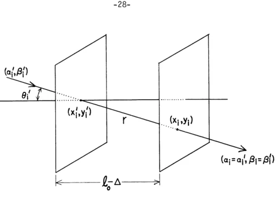
1.1 Problem Description and Geometry
The basic physical situation and coordinate system is shown in Fig. 1-1. There are two simplifying assumptions built into this descrip-tion. First, propagation is assumed to be horizontal. There is no attempt
TRANSMIT PLANE LASEF R ECEIVE R PLANE SCATTERING MEDIUM RECEIVER
Fig. 1-1 Physical Configuration of Underwater Channel
to deal with vertical or skewed transmission, either through different iden-tifiable ocean layers or through the air/sea interface. The air/sea inter-face is really another problem entirely. Furthermore, Himes has shown7 that transmission through different ocean layers can be described as a sim-ple extension of the one-layer results. Besides, the completely horizontal application has some very important applications, not the least of which is
the case of an untethered ocean vehicle transmitting laser data to a teth-ered bottom station.
The second assumption is that there are no gross inhomogeneities in the channel. There is no attempt to deal with events like the passage of a school of fish between the transmitter and the receiver, turbulence or "clumping" of particles to produce a large density gradient. The assumption is that this is an infrequent occurrence and that when it does happen,
transmission is temporarily disrupted. Of course, the medium is still con-sidered inhomogeneous because of the existence of randomly located scatter-ing particles. They are simply assumed to be uniformly distributed on the average for the present problem.
Note in Fig. 1-1 that the coordinate system has its origin at the receiver. Note also the coordinates a and
B
next to the usual cartesian coordinates x and y on the receiver plane. These are used to designate the angle of the incoming light relative to an orthogonal angular coordinate system. The orthogonal angular coordinates are obtained by a change of var-iables from the standard spherical coordinates. They are used here because the theoretical results that will be cited' are expressed in terms of them. They were originally chosen because they allow for valuable simplificationsin the derivation of the propagation equations and the final expressions obtained are also simpler.
The transformation involved is shown in Fig. 1-2. As seen in the figure, the transformation is a mapping of the unit-radius sphere onto a plane tangent to the sphere at
6=0.
(The plane in the diagram is drawn away from the sphere for the sake of visual clarity.) The mapping described preserves azimuthal angles $ and polar arc lengths. It converts two anglesa P 0
P
2----
7
-3vFig. 1-2 Mapping of Unit Sphere onto a-B Plane
to an angle and a length. The length, 6, of ~P in the a-B plane is the same as the arc length of OP on the unit sphere. The orthogonal angular coordinates of the point P are
a = ecos$ radians
(1-1)
= sin$ radians
Note the similarity between this transformation and the transformation of cartesian coordinates (x,y) to the ordinary polar coordinates (r,6) in two
dimensions.
1.2 Definition of Terms and Single Scattering Results
The greatest difficulty in dealing with the underwater optical channel theoretically lies in characterizing the process of multiple-scattering. Over any reasonable channel length there are enough suspended particles so that the incident light is scattered not once, but many times,
between the transmitter and receiver. Because of the random locations of the particles and their randomly distributed sizes, an exact description is impossible. And even a description of the average scattering behavior is quite complex.
There have been two basic approaches to the solution of the multiple-scattering problem. One is the use of linear transport theory'2. The main
product of this theory is a complicated integro-differential equation for the optical parameters of interest. While it has the advantage of including all relevant propagation processes, its main drawback is that it is
insol-uble except in some special cases. Arnush' was successful in getting tract-able results with this theory by making some simplifying assumptions.
For-tunately, these assumptions are applicable in the case of underwater optics. Karp' has shown that predictions from Arnush's results are in substantial agreement with measurements made by Duntley''.
The second approach to the multiple-scattering problem was intro-duced by Heggestad'. He divides up the multiple-scattering medium into a series of parallel layers perpendicular to the direction of propagation. Each layer is thin enough so that only a single scattering takes place within that layer. By calculating the optical response to a single typical
layer, and then superimposing the responses to the various layers in the medium, he obtains a simple expression for the "impulse response" of a scattering medium. While Heggestad's results were derived specifically for the atmospheric propagation problem - and will have to be modified slightly to apply to the underwater case - his simple physical approach, coupled with the fact that his theory is in the language and context of communication engineering, makes it more desirable to use his theory than
that of Arnush. Of course, both theories - if they are adequate descrip-tions of the physical situation - must produce the same results when trans-lated into the same terms. Karp9 has suggested that this is indeed the case.
Both of the above theories have their foundation ultimately in the results from single-scattering theory. The main result of this theory is that scattering from a particle can be characterized by a function called the scattering function, which measures the angular distribution of light scattered from a particle subject to an incident plane wave. The function
is denoted by Fr (6), where
e
is the angle between the incident plane wave and the direction of propagation of scattered radiation. The subscript, r,is the particle radius, and is included to stress the fact that this func-tion depends on the radius. The funcfunc-tion is defined in such a way that the intensity of light scattered into the solid angle dw is given by Fr ()dw, when the particle is illuminated by a unit-intensity plane wave.
In the present case, the particle sizes of interest are much larger than the incident light wavelength. (The experiment will utilize a helium-neon laser whose wavelength is approximately 0.6p. The particle sizes of interest in sea water range from 2-100p".) For this situation, single-scattering theory predicts a very sharply forward peaked single-scattering pattern. Furthermore, this sharp forward peaking has been experimentally verified by optical oceanographers". This characteristic of the single-scattering pattern was exploited by both Arnush and Heggestad in the development of their results. This was the simplifying assumption which Arnush made in order to solve the transport equation. Heggestad incorporates it into his derivation by defining the forward scattering pattern as
F r(0) |6| <
Ff,r(e)
=
2
(1-2)
0 elsewhere.
So far, the single-scattering pattern has been restricted to des-cribe scattering from a single particle of radius r. In any multiple-scattering medium, there are likely to be particles with a large range of
radii. Thus, an average forward-scattering pattern for the particles in the medium is defined as
Ff(f) =f Ffr(6)p(r)dr, (1-3)
0
where p(r) is the probability density function for the particle of radius r. A few words should be said about where this function p(r) comes from.
For decades, physical oceanographers have been making measurements of par-ticle size distributions in various samples of water from oceans around the world". The distribution function p(r) is simply a normalized version of a typical measured particle size distribution. Although there are
var-iations in this measured distribution from ocean to ocean, when integrated against F (6) and normalized to the value Ff( ) the scattering patterns
f,rf2
are all remarkably similar. (See the Appendix for a discussion of this issue.)
To account for situations in which the total amount of scattered light is different, Heggestad defines the normalized average single-particle forward-scattering pattern as
f(e)
= .fe (1-4)Because this function normalizes the scattering function to the total
amount of scattered light, if f(e) is different in two physical situations, it is due to the difference in relative distribution of scattered light, and not to the fact that there was more total scattered light in one sit-uation than in the other.
Heggestad's results do not actually depend on an exact specification of f(e), but only on the width of f(e). In the development of his theory, Heggestad defines two quantities W2 and W2 as measures of the width of f(6) in orthogonal angular coordinates. These quantities are analogous to the marginal variances of a joint probability density function. They are
de-fined as
W2 = fdada2f(a,6)
Ot (1-5)
W2 = dad662f(a,),
where f(a,) = f(/a2 + 2) since e2 = a2 + 32 by the transformation
equa-tions [Eq. (1-1)].
The other parameters that will be of interest in the discussion below are the absorption coefficient and the scattering coefficient, desig-nated by
a.
and 5, respectively. The absorption coefficient is the optical power absorbed by a medium per unit volume per unit incident intensity (or the power absorbed along the length of a collimated beam per unit length per unit incident power). The scattering coefficient is the total optical power scattered from a medium per unit volume per unit incident intensity(or the power scattered out of a collimated beam per unit length per unit incident power). Physical oceanography shows that on the average these two quantities are constants in a uniform medium and characterize that medium's
optical properties. Assuming that scattering and absorption are the only two means by which light can be removed from a given volume of water, then clearly the total power lost from the medium per unit volume per unit inten-sity must be 0.+5 This quantity is called the extinction coefficient and
is denoted by c.
The coefficient c is frequently expressed as the reciprocal of the "extinction distance," denoted by De* This quantity is the distance a plane wave must travel through a medium before its intensity is down by l/e
from its initial value. When distance within the medium is normalized to De, it is called optical thickness, and denoted by Ne. Thus,
N e T (1-6)
D
e
is the optical thickness of the medium between transmitter and receiver. Only one more quantity need be defined here. It is called the aver-age forward-scattering efficiency, denoted by yf, and it is the proportion of the total extinguished light which was scattered forward and not absor-bed. Thus
Y
a
C
c-a (1-7)
With the above definitions, we now have the conceptual paraphernalia to describe the major results and techniques of the scattering theory devel-oped by Heggestad, and to modify them appropriately for the present phys-ical context.
CHAPTER 2
SCATTERING THEORY RESULTS AND MODIFICATIONS 2.1 Power Distribution Function
Those aspects of Heggestad's theory which are applicable to laser beam propagation are presented in terms of the transfer of the power dis-tribution function, P(a,,x,y). It's dimensions are watts/meter2-steradian.
This function is defined by the statement that P(a,6,x,y)dadedxdy is the total power borne by those rays of light with angles of arrival in a solid angle dad at the angular position (a,6) which falls on an area dxdy at the point (x,y) on a plane parallel to the receiver plane. See Fig. 2-1.
y
dad
(a,13) x
Fig. 2-1 Geometry for Definition of Power Distribution Function
(The power distribution function is nearly equivalent to the standard def-inition of radiometric "radiance," except that radiance uses an area dxdy which is perpendicular to the incoming ray at (a,8).)
length of the medium that the light traverses.. But it is clearly specified everywhere along the way in the discussion below. (It is the channel
length T in Fig. 1-1.)
2.2 Results from Scattering Theory
The scattering/absorbing processes are linear processes, and while multiple scattering is a random phenomenon, Heggestad shows that on the average, the scattering medium has constant optical properties". This means that the underwater medium can be treated as a two-dimensional linear system, and all the ideas of linear system theory can be used to calculate average optical responses through the medium. In particular, the medium
can be entirely characterized by a single function, the impulse response, designated by hp (atq,x,y;a , ),x0yo). This function is the power distri-bution function response at coordinates (a,f,x,y) on the receiver plane to
the impulsive power distribution function
Pi(a,6,xy) = u0(Oc-aa)uo(-S)uo(x-x)u0(y-y0 ) (2-1)
on the transmit plane.
The main result of Heggestad's theory is the specification of this impulse response as the four-dimensional jointly Gaussian function'5
exp[-N e(1-y )]
h
p(a
qI,x,y;Ct
, ,x ,y)
= e( 1 YI
-a0)2 (-a )(x-x 0+Ta0) (x-x 0+Ta 0 2
exp -2 a2_+_ 4 0 +2 (2-2) 6- Ota x x ( 0- )2 (6- 0c (y-yo0+1[6 0) (Y-y0 +T 0 2 exp -2 _ _+ 0 ] y
2
C2
where
2 = yNwa2 2 T 2
rtfe a X 3 ct
2 =YNw 2 a2 = 2 (2-3)
The quantities yfg W2 and W2 are the single-scattering parmeters defined
in Chapter 1. The quantity T is the channel length, and Ne is the optical
thickness from transmitter to receiver.
2.3 Modifications for the Underwater Problem
Since Heggestad's results were derived for the case of multiple-scattering through an atmospheric channel, it is appropriate to ask whether or not they are directly applicable to the underwater environment. Himes has pointed out'6 that certain modifications need to be made to the theory
to make it usable underwater. The main reason for this is that Heggestad treats the optical propagation problem in such a way as to ignore the fact that light which is scattered is also absorbed. He breaks up the light field into three parts: that part which is scattered but not absorbed, that part which is absorbed but not scattered, and that part which traverses the medium without having been scattered or absorbed. These three compon-ents may be all that is necessary in the context of atmospheric channels, which are very mildly absorbing (so that the extra path-length introduced by scattering does not significantly change the quantity of absorbed light).
But in the underwater case, the absorption is a much larger percentage of the overall extinction, and thus the absorption of scattered light cannot be ignored.
will affect the prediction of the angular spectrum. If none of the light that gets scattered out to large angles is absorbed, then all of that light must reach the receiver. Hence the predicted angular spectrum based on this assumption of no absorption will be broader than the actual one. If the absorption of scattered light is taken into account, the theory
pre-dicts that much of the light that gets scattered out to large angles will be absorbed long before it ever gets to the receiver. Hence, the predicted angular spectrum will be narrower than it would have been if this effect
had been ignored. The actual magnitude of the difference will be explored at the end of this chapter.
Himes suggests a method of modifying Heggestad's results to include the absorption of scattered light. He applied this method to the special case of a plane wave propagating through the underwater medium. The same basic method will be used here to extend these results to the complete power distribution impulse response function, hP (). This will give a mod-ified form of h p(-) which will be applicable to the underwater transmission of laser light.
As stated in Chapter 1, Heggestad begins his derivation by dividing the scattering medium into N thin layers, each of thickness k0. This is pic-tured in Fig. 2-2. The assumption built into this approach is that each of these layers is thin enough so that only single scattering takes place with-in a layer. Furthermore, the thinness of the layer makes it possible to treat it as if all the scattering particles were distributed on a single plane rather than in the volume of the layer. Heggestad computes a spatial
impulse response for a single layer and, using as the input to each subse-quent layer the output of the layer before it, he convolves the (N-1)
*th
I LAYER
LASER RECEIVER
Fig. 2-2 Thin Scattering Layer Description
single-layer impulse responses to get an overall N-layer impulse response. He completes his derivation by taking the limit as to + 0 and N + oo, while
keeping Nko = T constant.
The thin-layer approach will be followed here too, except that to account for absorption each single layer will be broken up into two sub-layers, one in which there is only scattering, followed by one in which there is only absorption. The geometry of a typical layer is pictured in Fig. 2-3. The coordinates, both angular and spatial, are written for each segment of the i th layer.
Consider computing the impulse response of the ith complete layer. The scattered light output of the scattering sub-layer is identical to the scattered light output of a layer as computed by Heggestad, since in both cases there is no absorption in the layer. Heggestad's derivation entails calculating the response to the hybrid incident distribution
PURELY PURELY ABSORBING SCATTERING SUB-LAYER SUB-LAYER ALL SCATTERING ASSUMED TO OCCUR ON FRONT (ai~j,8i-1;xi-i'yi-) , , SURFACE (ai,#i'sx;~,y;') OF LAYER (aj= a',S;=R;',xjjy;)
Fig. 2-3 Geometry of ith Layer
P(a~,r,x,y) = uo (-aL )u (M-65_)
= 0 i1 0 -i ) (2-4)
u_l(x-x )u l(y-y _ ),
where he has replaced two of the impulses in Eq. (2-1) by step functions for simplicity of calculation. To get the impulse response, he takes par-tial derivatives with respect to x and y of the response to this hybrid distribution. This approach is valid here and the same reasoning will be followed, with appropriate modifications along the way.
The average scattered power at the output of the scattering layer is identical in form to Heggestad's expression [See Reference 1, Eq. (3-83).]:
outscattered(a ,1',ixi',y g 'a ,Sgi- xi- !y ) =
SAsece6. f(a 'i-l , i-l) (2-5)
Here A is the scattering sub-layer thickness, f(-) is the average normal-ized single-scattering function, and S is the average scattering coefficient defined in Chapter 1. (Heggestad derives his results in terms of the aver-age scattering cross-section, C and the volume particle density of a
layer, dv. I have chosen to keep the notation of the average scattering coefficient for simplicity. The scattering cross-section is related to the scattering coefficient by the expression S = dvC~.) Note also that, as indicated in Chapter 1,
6i =
/2
+ 62 (2-6)As in Chapter 1 the mixture of spherical and orthogonal angular coordin-ates will be maintained in the derivation for the obvious notational con-venience.
While it has been possible to use Heggestad's expression for the average scattered power virtually intact, his expression for the average unscattered power will have to be changed. The reason is that the present derivation assumes no absorption at all in the scattering layer (saving it all for the absorption layer), whereas Heggestad included the absorption of unscattered light in his derivation. But by following his derivation care-fully it can be seen that this manifests itself only in his use of the extinction coefficient, c (or more precisely, in his use of the extinction cross-section Cext = C/dv). What he is saying is that the amount of light power that reaches the end of the scattering layer without having been
scattered is decreased from that of the input by the total light extinguish-ed (scatterextinguish-ed and absorbextinguish-ed). Thus for the present case, this neextinguish-ed only be modified to say that the amount is decreased by the amount of light
scat-tered, since here only light which is scattered doesn't make it out of the scattering sub-layer. This is accomplished by replacing the extinction coefficient by the scattering coefficient. With this change, Heggestad's
Eq. (3-84) becomes
Pout~unscattered~ai', ',I,,;ggS~~ Ix) _ ,y
(1-SAsece_ -) sec6e i- cosei 'u 0(ag ' - ~ ) (2-7)2-) u 0(N3 'i- )u_ (x '-x _ +a 'A)
u_3 (yi '-yi- _+65 'A)dodxdy .
From here, the derivation proceeds exactly as in Heggestad, so that the scattering layer impulse response is
h s(ag ',65',I xg'y 'a ~ ,5g x~ ) =
[(1-SAsce _ )u 0 (a
('O-a _ )uU(3'
-l) + (2-8)
u 0(xi '-1_+a 'A)u O(yi '- + i'A).
Here, sec 6il_ is defined as
sec6..1 < sec~1
sec =w ls (2-9)
1- 1l el sewhere.
This approximation to sec
eil_
is made throughout Heggestad's work in order to insure that the impulse response does not become negative. This is in accord with the assumption that there is no appreciable backscattered light from the i th layer, and Heggestad analyzes the limitations placed on theapplicability of the theory by this assumption. (The most important limit-ation is that the theory cannot be used for optical thicknesses, Ne, great-er than 30. For optical thicknesses this large, even though the light
scattered from a particle will have no appreciable component in the direct-ion from which it came to the particle, there is no guarantee that that direction is not close enough to Tr/2 to make the cumulative scattered angle negative.)
To obtain the output of the absorbing part of the i th layer, refer to Fig. 2-4. The distance that the ray traverses through the layer is
P, -A
r 0
7cos- (2-10)
= (, 0-A)sece'
Thus, the power loss through the layer is in accordance with the exponen-tial absorption law,
rout
-(
U-A)sec6.'t , (2-11)in
where a is the absorption coefficient of the medium. (It should be noted here that to the extent that a medium has significant backscattered light, the coefficient in the above expression would have to include this back-scattered light as an average total loss per unit distance, and thus the use of the absorption coefficient would not be accurate. It is an assumption of this thesis, however, that there is no significant backscattered light.)
Note from Fig. (2-4) that the coordinates (x ,y ) of the exit point are not the same as those of the incident point on the layer. The relation
2-A
0
Fig. 2-4 Geometry of Absorbing Sub-Layer
x = x+(k -A)a
1 1 i
Using Eqs. (2-11) and (2-12), and the fact that
the output of the absorbing layer can be written
h(a ,f3. ,x. ,y ;i- )i ,xi 1 ,yi-l) =
exp[- (-A)Asece ][(1-SAsece._ )uabo -ai_ )
uO9 -6 _ )+5Asece. _ If(ai- -_ ,I.-5_
uob
i-x- _k
0
a
i)uO(yi-yi-l+%Y)
(2-12)
(2-13)
(2-14) (ai=ai,#i=8!)
This is the impulse response of the ith layer of the underwater medium. To obtain the impulse response of the entire medium, we proceed as in Heggestad to construct the (N-l)-fold superposition integral
hN
(NON'NYN;o
O,,
x0,yO)
= f-
-da N-1
.. da 1f-
.f
dN-
1...
dff
...
SdxN-1 ...
dxf . dyN- 1
...
dy
(
[h(aN'3x N'JyN;'N-l' N-l'XN-l' N-l '-5 h(a s,6 ,xa ,yg ;a 3,S 5x 5yo)] .
Now since the single-layer impulse responses are very similar to those cal-culated by Heggestad, the product of these impulse responses in the above integral will be identical to that of Heggestad except for two things:
(a) The extinction coefficient is everywhere replaced by the scat-tering coefficient, and
(b) There is a product term of the form
exp[-( 0-A)sece1
a-...-(z
O-A)secN1N (2-16)
exp[-( 0-A)aEsece.]
i=1
in front of the N product terms in the integrand.
Note that this exponential term cannot be taken out of the integral because the
e.
are functions of the (oqf). But this term can be simpli-fied by using the fact that the scattering is very sharply forward peaked. The summation in the exponent can be re-written asN N/2 secO. N sec6e
E secO. = sece Z 1 + seceN E , (2-17)
i=l i=l sec6
and because of the sharp forward peaking, sece. secO. - =1 (2-18) sece seceN Thus, N
Z
sece. ~ (sece1+seceN) (2-19) i=l1 2By the same sharp forward peaking argument above, it is clear that cannot be that much different from eO, so that
N
Z sece - (sece0+seceN) (2-20)
1=1 2
Note that this expression no longer contains any of the variables of in-tegration, and thus the exponential
N
exp[-(Z -A)a.
z
sece6] =i=1 (2-21)
exp[-2 ( -A)a(sece0+seceN) *
can be pulled out of the integral.
What is left in the integral is identical to the expression
Heggestad used except that the extinction coefficient is replaced by the scattering coefficient. But inspecting Heggestad's derivation and his final expression [Eq. (2-2) above], the only place this coefficient appears is in the first exponential term,
(2-22) exp [- N e(1-y)] .
Recall from Eq. (1-8) that
-S
Yf - (2-23)
and if c is replaced by S, this becomes 1, so that the exponential term becomes 1. But note that while that exponential term (which was supposed to account for absorption) drops out of the expression, the present deriva-tion includes another one: the impulse response must be multiplied by Eq. (2-21).
Consider this new exponential term in the limit as (k -A) approaches zero and N approaches infinity. Since N. = T is held constant as the limit
is taken, and since A -+ 0 faster than k 0 does, exp[--N (9-A)a.(sec 0+seceN)]
2 0(2-24)
exp[- -I-
0,(sece0+seceN)1
2in the limit. It will be instructive to cast this expression in the same terms as Eq. (2-22). To this end, write
Ta. = N D (E-3)
= N D e(1- ) (2-25)
= Ne (l-yf)
since D e = 1. Thus the new exponential term is
sec6 +secO
exp[-Ne(l-yf) 2 (2-26)
2
reason to keep the subscript N.
It should be clear from this expression exactly how Heggestad's results have been modified to apply to the underwater problem. His expon-ential absorption term [Eq. (2-22)] was inadequate because it did not in-clude the absorption of light scattered to non-zero angles. The new term, Eq. (2-26), includes these effects by multiplying the exponent by a func-tion of the angular spread. This funcfunc-tion,
secO +secO
0 , (2-27)
2
is the average of the secants of the input and output angles. Multiplying by this term amounts to using the average value of the path-length as the effective optical thickness of the channel. While it is not strictly cor-rect because it ignores the zigzagging that a ray of light might actually undergo as it traverses the medium, it has been argued above that the sharp forward peaking of the single-particle scattering function implies that deviation from the average will be small. Thus Eq. (2-26) should give a sufficiently accurate correction to Heggestad's results to be adequate for the underwater problem.
Using Eq. (2-26), the final expression for the power distribution function impulse response can be written as [compare with Eq. (2-2)]
=exp[-N (T-y)(sec6+sece h(at,8,x,y;a, 3 O,x ,yO) -e fJ 2
- 2(2-28 )
exp -2 0a +3aa )(XO+Ta) +X__o+Ta____ + Vk
exp -2
~ o+((yTo)()
+ (Y~ 0+T2) . (2-28 cont.)2 Y &l 2
Here the parameters are the same as in Eqs. (2-3).
In the context of the present work, Eq. (2-28) can be simplified. The light source will be a laser oriented in the zero direction with neg-ligible angular dispersion and negneg-ligible beamwidth. Thus a = 0 = 0= 0.
Also the laser beam will be centered on x = y = 0. Incorporating this into Eq. (2-28) gives 1+sece h(c,,x,y;O,0,0,0) = exp[-Ne(l-yf)( 2 Tr 2aaCx
a,
(2-29) exp[-2( + + 2]ex[2 +/3 $) Cy2C C )]x[2
+V 3y a Ox x Cr X Cy 'yThis expression can now be used to predict the angular distribution of light at the output of the medium due to the laser source input, since the laser is effectively an impulse. To obtain the absolute power level, it is only necessary to multiply Eq. (2-29) by the laser input power, P
0. It should be noted at this point that the theory as described here is limited in two respects. First, by the nature of the limiting process described above, the theory is only valid for optical thicknesses larger than five. The reason for this is simply that for smaller optical thick-nesses the superposition integral does not converge to a Gaussian. This issue is discussed in detail by Heggestad'. The second limitation of the above theory is that it neglects light which is not extinguished at all in traversing the medium. But this can be added in easily by adding to
Eq. (2-29) an impulsive term whose magnitude is e- Ne
2.4 Comparison of Atmospheric and Modified Theory
It is now possible to explore the actual magnitude of the difference between Heggestad's theory and the modified version derived here. One dimensional angular spectrum plots for a representative optical thickness of 25 are shown in Fig. 2-5, for increasing values of yf. Note that, as expected, the two theories give very similar results at small angles, and that the modified version consistently predicts a narrower angular spectrum. Furthermore, the two theories converge as yf approaches 1. It is apparent from the curves in Fig. 2-5 that the two theories are not significantly dif-ferent for angles less than 300. Although the divergence is much greater at angles close to 90' there is negligible power at those angles. The ex-periment described in the next two chapters explores only the small angle behavior.
-35-ATMOSPHERIC THEORY MODIFIED THEORY Fig. 2-5a yf = 0.7 4 8 12 16 20 24 28 ANGLE (0) . ATMOSPHERIC THEORY Fig. 2-5b yf = 0.9 0 4 8 12 16 20 24 28 ANGLE (0) Fig. 2-5c yf = 0.95
Fig. 2-5 Angular Spectrum Plots: Comparison of 2 Theories
Ld L)
z
M .0 0-100 80 60 40 20 O L 0 100 80 60 40 20 0 100 80 60 40 20 01 0 4 8 12 16 20 24 28 ANGLE (0)CHAPTER 3
DESCRIPTION OF EXPERIMENT
The purpose of this chapter is to describe an experiment designed to simulate an undersea optical channel on a small scale, and to measure the angular spectrum at the receiver end of the channel. In addition, measure-ment techniques for the absorption and extinction coefficients will be described, since knowledge of these is necessary in order to correlate the experimental results with the theoretical predictions.
The main goal of the measurement program is to measure the angular spectrum on and off the optical axis of the laser beam for optical thick-nesses, Ne, between 5 and 10 and for a variety of forward scattering effi-ciencies, yf. The lower limit for the optical thickness is set by the range of validity of the theory, as explained in Chapter 2. The upper limit is
set by absolute detector sensitivity of the available equipment. The values of yf and Ne are controlled by the relative proportion of dopants in a tap-water-filled tank.
3.1 The Channel
The channel is a steel tank, measuring 3 feet by 3 1/2 feet by 4 feet with two windows on one end: one halfway down the wall and the other about six inches from the top of the tank. The tank is painted flat black to avoid any reflections from the walls that will interfere with the measure-ments. Initially there was some concern about whether the light absorbed by the walls was actually affecting the measurements: in a preliminary study conducted in a smoke-filled chamber", it was observed that the opti-cal field died out half-way down the chamber for heavy doping. This
ap-peared to coincide with the point at which the width of the beam reached the walls (the chamber was twice as long as it was wide). While it was not possible to determine the cause and effect relationship in this case,
(although some complaints from Duntleyl1 support the view that the walls interfere), it was decided to make the underwater channel not much longer than it was wide. Aside from the ready availability of such a tank at the start of this program, this was the main consideration that dictated the choice of the tank size.
The channel is doped with two chemicals to simulate the ocean en-vironment. One is a scattering agent called Alurex, which is a suspension of magnesium and aluminum hydroxides. It is one of a number of "stomach gels" made by Rexall, and it was found by Duntley" to be the scattering agent which produced a single-particle scattering function closest to that of natural waters. (He called the product Aluminox, which was its previous name.) The other chemical used in the doping of the channel is Nigrosin, a water soluble biological stain produced by MCB Corp. Nigrosin produces no scattering but is a pure absorbing dye.
The reason that two inert chemicals are used instead of trying to synthesize a small-scale biological environment is that the latter re-quires a very careful balance of nutrients and very careful control of temperature, salinity, etc. It was not feasible to attempt this in an experiment of this scale. Furthermore, using two chemicals allows com-pletely independent control over both the absorption and scattering in the tank. This is desirable so that light transmission can be measured at any mixture of absorption and scattering, or saying it another way, any value of Yf.
3.2 Angular Spectrum Measurement
The angular spectrum is measured by keeping the laser source fixed and by rotating a narrow field of view photodetector. The source is a Spectra Physics Model 132 He-Ne laser at 6328
A
with a nominal power of 1.0 mwatts. At the 1/e2 points on the beam, the beam diameter is 0.8 mm and the beam divergence is 1.0 mradian. (As stated above, these dimensions are negligible compared to the size of the output field's angular and spa-tial width. See the Appendix for further discussion of this issue.)The receiver is an EG&G Model 550-1 radiometer. This instrument consists of a photodetector head with associated optics attached to a dig-ital readout via a cable. When used with a standard lens attachment and associated filter, the Model 550-1 directly measures radiance (power per unit solid angle per unit area perpendicular to the face of the detector). Unfortunately, the standard lens attachment provides an 8' field of view (FOV), which was deemed too wide for this application. Thus some conver-sions will have to be made in the measurements. This will be discussed in Section 3.2.2.
3.2.1 System Structure and Alignment
Both the laser and the photodetector head are mounted on a rigid wooden bracket. This is necessary in order to have accurate alignment of
the receiver axis with the laser beam axis. (Accurate alignment was found to be the most necessary capability of the system in the smoke channel ex-periments referred to above' 7. It was also found to be the most difficult
to achieve.) A diagram of this structure in position on the tank is shown in Fig. 3-1. Note that the laser is fixed in place out of the water on the
OPTICAL TRACK
LASER'
PIVOT
DETETOR
ROD
DETECTOR
ROD
HOUSING
Fig. 3-1 Structure for Angular Spectrum Measurement
overhanging "L". It points in through the lower window toward the detec-tor which is under water and enclosed in a water-tight vessel.
The vessel is connected to the optical track by two rods inserted in moveable slides on the track. The front rod is located at the point around which the detector is pivoted. This pivot point is directly above the lens attached to the detector head. The purpose of placing the pivot point here is to insure that the laser beam passing through the center of the lens will not be deflected as the detector is rotated.
The rear rod is used for the purpose of rotating the vessel. It is attached to a slide which is free to move laterally across the optical track. As the rear rod is forced to the side by the lateral motion of this slide, the detector is rotated. This process is shown in Fig. 3-2. The rear rod can also be moved vertically up and down and thus also serves
Fig. 3-2 Schematic of Lateral-to-Angular Conversion (Top View)
the purpose of changing the elevation angle of the detector for ease in alignment. All told, the detector assembly has 5 degrees of freedom: It can move along the length of the optical track, laterally across the track, vertically, the azimuth angle can be changed, and so can the elevation angle.
The structure was designed so that everything could be mounted as one solid unit and could be taken off or returned to its position on the tank at will. It was thought that this would make it possible to align the system when it is completely out of the water. This turned out to be unfeasible for two reasons: First, the structure was too heavy to remove from the tank easily; second, the difference between the refractive inde-ces in water and air was enough to cause the system aligned in air to be non-aligned when placed in water. It was still possible to align the system with clear water in the tank. To do this, two rods with small holes in them are hung down from the optical track, one near the laser and the other near the detector (see Fig. 3-3). The laser is then positioned so that the beam goes through the two holes and gives a peak response in
Fig. 3-3 Alignment Procedure
the track. The two rods can be removed when a measurement is to be made. As pointed out in the smoke-channel report", this alignment procedure is not a one-time affair, but must be carried out periodically.
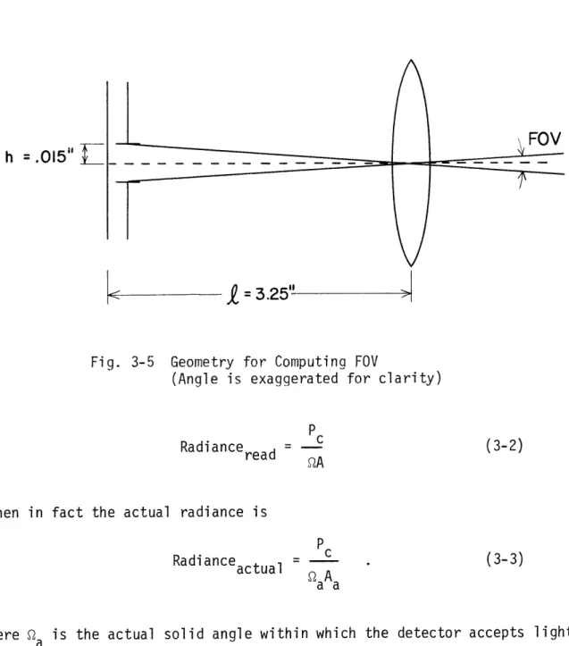
3.2.2 Detector Optics
A diagram of the detector optics is shown in Fig. 3-4. Without the field stop, the lens/filter combination is a standard attachment to the EG&G 550-1 radiometer. This combination of lens and filter is calibrated to give a readout directly in pwatts/cm2-steradian. Unfortunately, how-ever, the system has an 8* field of view (FOV) and a 1 7/8" aperture with this combination. As shown in the Appendix, the full angle FOV should be at most 10 and the aperture diameter should be at most 0.084" in order that there not be a substantial change in the light field within the FOV. Thus it was necessary to place a field stop pinhole in front of the detec-tor surface and an aperture stop behind the lens.
A pinhole of 0.03" was readily available. The FOV produced with this pinhole can be obtained from the expression
DETECTOR
SURFACE
LENS 0.09" APERTURE "FLAT" 0.03" DIAMETER FILTER FIELD STOP
Fig. 3-4 Schematic of Detector Optics
FOV = 2tan~ I (3-1)
(Refer to the geometry in Fig. 3-5.) The FOV is .55', which is less than the maximum allowed of 10. The aperture size was drilled to a standard size of 3/32", or .094", which is just slightly larger than the maximum required aperture of .084".
Since the FOV and aperture are much smaller than that for which the EG&G 550-1 was designed, it will not read the actual radiance directly. A correction factor must be applied to the readings. To obtain this correc-tion, note that the detector computes the radiance by dividing the total collected power, Pc, by the product QA, where Q is the solid angle in which it accepts light with the 8* FOV, and A is the area of the lens aperture. Even though the system aperture and FOV have been changed, the system still calculates
h =.015"
<3.25"
Fig. 3-5 Geometry for Computing FOV
(Angle is exaggerated for clarity)
P
Radiance read c (3-2)
QA when in fact the actual radiance is
P
Radiance actual c (3-3)
a~a
Here Qa is the actual solid angle within which the detector accepts light with the 1/20 FOV and Aa is the area of the .094" diameter aperture. Thus,
Radianceactual = Radianceread . (3-4) a a A a Now A d (3-5) 22
where Ad is the area of the EG&G 550-1 detector face (1 cm2, or .155 in2) ,
and k is the distance between lens and detector. And A
a k2 (3-6)
where A is the area of the field stop pinhole. geometry described.
Ad
Refer to Fig. 3-6 for the
A
0Fig. 3-6 Detector Optics Modifications Geometry
Substituting Eqs. (3-5) and (3-6) into Eq. (3-4) gives
Radianceactual A = (1 7/8" )2= 2.76in 2 4 A d = .155in,2 A A = Radiance d read -A = 094) 9 2= .0069in. 2 a 4 Ap= Tj(.030")2= .00075i n. 2 Since (3-7) (3-8)
this becomes
RadianceacRadanceadianceread 82,667 (3-9)
The factor 82,667 was used as a correction to all of the radiometer read-ings.
3.2.3 Measurement of Optical Thickness
It is necessary to measure the optical thickness, Ne, of the medium in order to correllate the experimental results and theoretical predic-tions. To do this, note that the light that is extinguished is either scattered out of the beam or absorbed. Thus a very narrow angle FOV mea-surement of on-axis radiance will collect all the power which has not been scattered or absorbed. The power collected is then
P = P e~ c cal T
(3-10)
(-0Here e is the extinction coefficient and T is the channel length. Pcal is simply a constant which depends on the boundaries and the input power. It is to be determined by a calibration measurement.
To make the calibration, another measurement is taken with clear water in the tank. The reason that the calibration is made with water in the tank, rather than making it in air, is that the water-glass
boundar-ies must be the same for both the actual measurement and for the calibra-tion. Otherwise significant errors may result from reflections at these boundaries which are not accounted for. If the calibration measurement
is made right at the input window to the tank, while Pc is measured at the desired range, then Eq. (3-10) can be used to calculate the total optical
thickness of the water (including the very small value due to extinction in clear water), as Ne = CT = in -cl (3-11) P c 3.2.4 Measurement of Angle
The angle measurement was not a trivial matter. A number of me-chanical schemes were tried initially (eg. correllating the angle with the number of rotations of the lateral motion screw on the rear optical bench bracket), but none of them were able to achieve the 1/20 angular tolerance needed for the measurements. Finally it was decided to use an optical
method: a second laser sent a beam of light through the upper tank window (above the water level) and reflected off a mirror mounted to the detector pivot rod. The reflected beam put a spot on a ruler mounted on the side of the tank wall, and the ruler reading was related to the angle of rota-tion. This scheme is shown in Fig. 3-7. The conversion from ruler read-ing, x, to angle is
= tan~1(- ) . (3-12)
3.3 The Absorption Meter
It is necessary to have an accurate measurement of absorption to compare the experiment with the theory. There are essentially three ways
to do this. The first involves using a laser source and collecting all the scattered light at the receiver with a large collector. Clearly if all the scattered light is collected, what was not collected had to be absorbed (except for a small backscattered component which was shown in Chapter 1 to be negligible). The problem with this method is that it requires a large collector to collect all the scattered light. And how large is "large" depends on the amount of light scattered. The dilemma is that it is necessary to calculate the scattering profile at the receiver, in order to accurately make a measurement which is to be used to verify the theory underlying the calculation! It would be possible, of course, to use a huge collector which would eliminate any doubt, but this was not
feasible for this application.
A second method of absorption measurement was developed by Duntley", which involves use of the divergence relation for
irradi-19,i20
ance . While this method is very accurate, it involves the fabrica-tion of very sophisticated collectors which made it impossible to use in this context.
The simplest absorption measurement technique was developed at Stanford Research Institute2 1. This technique uses an omni-directional
point source and relies on the spherical symmetry to eliminate the effects due to scattering. That is, while there obviously will still be scattering in the medium, it will have no preferred direction if the inhomogeneities are uniformly distributed. The power collected by a photodiode of area AD at a distance r from a point source of power PO is
A
P = PO De- . (3-13)
A
The factor AD is the proportion of the total omni-directional power which is interrupted by the surface element AD lying on the sphere of radius r facing the point source. The absorption coefficient, a, could be obtained directly from Eq. (3-13), but in order to avoid having to know
the diode parameters exactly, a second measurement is made at another dis-tance in order to calibrate the reading. This procedure is discussed in the sections that follow.
3.3.1 Mechanical Design of Absorption Meter
The experience of the researchers at Stanford strongly points to the necessity of using two, rather than one, photodiode. They found that the accuracy of the absorption measurements was very sensitive to accuracy in the values of r1 and r2. Thus, instead of having a single diode which is moved to two locations for the two measurements, it was recommended
that two diodes be used to eliminate placement errors when moving the de-tector.
The absorption meter is constructed as a triangular frame with the two diodes rigidly fixed in place, and the point source between them. This is shown in Fig. 3-8. The frame is lightweight aluminum painted black and
DIODE
Fig. 3-8 Absorption Meter Structure
is suspended in the experimental tank from the apex. The size of the base, rI+r2 Vis limited to 3 feet so that it fits in the tank. It will be shown below, however, that there are more stringent restrictions on the dis-tances r1 and r2 imposed by the available source and detectors.
3.3.2 Electrical and Optical Aspects of the Absorption Meter
The source used for the absorption meter is a General Radio Type 1539-A "Stroboslave" which is a triggerable strobe. The two photodiodes
used are EG&G Type SD-100.
It is desirable to use a pulsed source for this application so that the high peak power obtained will allow for a reasonable signal to noise ratio (SNR). (SNR issues will be discussed below.)
The available source power is obtained from the Type 1539-A instruc-tion manual2 2 as 10' beam candles per pulse when used with a 100 beam.
The beam candle power (BCP) is the luminous flux per steradian emitted from a directional source2 3. Thus,
BCP - F (3-14)
where F is the power in lumens and Q is the solid angle of the cone in which the beam is contained. (The unit "lumen" used here is the optical power integrated over all wavelengths against the "standard luminosity curve." This curve is designed to convert actual optical power to a measure of visual brightness as perceived by human beings. In the wave-length region of interest here, there are roughly 680 lumens/watt.) The expression used to obtain the solid angle from the 100 beam-width is24
= 2'r(l-cosl 0 )
(3-15)
= .095 steradian
Using this value, the available power of the source (in watts) is
F = (10)7(.095)lumens(%o)lumen
(3-16) = 1397 watts
meter, it will be necessary to get an expression for the SNR of the photo-diode. Fig. 3-9 shows the circuit configuration used in the absorption meter and the equivalent electrical circuit of the diode itself25 . In the
STROBE R LAMP-F ILT E R .I|CL S DJ -- R B IAS~i L 4 VOUT
Fig. 3-9a Detector Circuit Configuration
Fig. 3-9b SD-100 Diode Equivalent Circuit
photoconductive mode, the SD-100 acts as a current generator. Considering the SNR as a voltage ratio then, the signal voltage is
S = ISR L (3-17)
where I is the signal current and RL is the load resistance. The two sources of mean-squared current noise are2
1:
a) Shot noise: i = 2q(I +I +I)Af b) Thermal Noise: i = 4kTAf
R S+RL