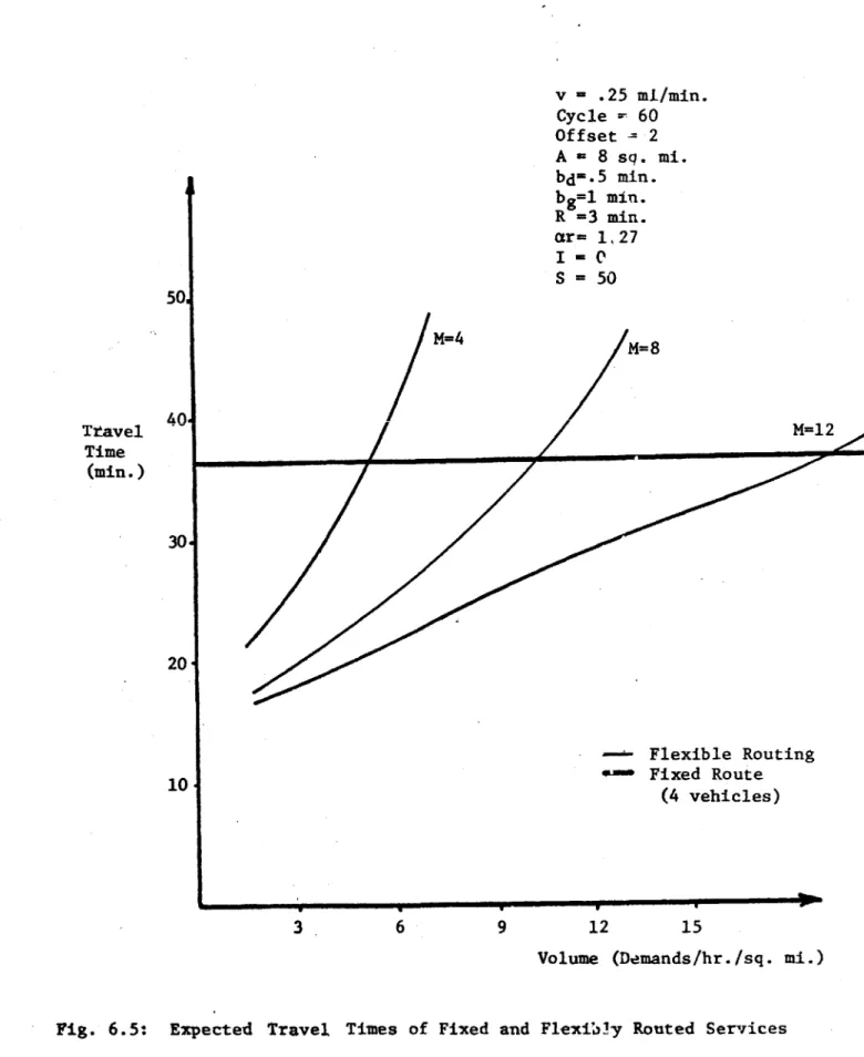
Approximate, analytic performance models of integrated transit system components
Texte intégral
Figure


Documents relatifs
Klibanov, Global uniqueness of a multidimensionnal inverse problem for a non linear parabolic equation by a Carleman estimate, Inverse Problems, 20, 1003-1032, (2004).
(1978) to estimate the entire genetic variance-covariance structure as well as the residual variance of the continuous trait only, and the residual covariance
Lastly, for problems with a very large number of classes, like Chinese or Japanese ideogram recognition, we suspect that the unbalance of the number of the
A simple kinetic model of the solar corona has been developed at BISA (Pier- rard & Lamy 2003) in order to study the temperatures of the solar ions in coronal regions
By a classical result of Chern-Moser [4], any formal biholomorphic transformation in the complex N-dimensional space, N > 1, sending two real-analytic strongly
If I could have raised my hand despite the fact that determinism is true and I did not raise it, then indeed it is true both in the weak sense and in the strong sense that I
Under the arrival process and service time distributions described in Section 3 and the parameter values in Table 3, we have validated our simulation model by comparing the
LCA is a method used to estimate the materials and energy flows – and the potential environmental impacts – of a product or service throughout its life cycle:
