A Comparison of empirical indoor relative humidity models with measured data

Publisher’s version / Version de l'éditeur:

Journal of Building Physics, 31, January 3, pp. 243-268, 2008-01-01

READ THESE TERMS AND CONDITIONS CAREFULLY BEFORE USING THIS WEBSITE.

https://nrc-publications.canada.ca/eng/copyright

Vous avez des questions? Nous pouvons vous aider. Pour communiquer directement avec un auteur, consultez la

première page de la revue dans laquelle son article a été publié afin de trouver ses coordonnées. Si vous n’arrivez pas à les repérer, communiquez avec nous à PublicationsArchive-ArchivesPublications@nrc-cnrc.gc.ca.

Questions? Contact the NRC Publications Archive team at

PublicationsArchive-ArchivesPublications@nrc-cnrc.gc.ca. If you wish to email the authors directly, please see the first page of the publication for their contact information.

Archives des publications du CNRC

This publication could be one of several versions: author’s original, accepted manuscript or the publisher’s version. / La version de cette publication peut être l’une des suivantes : la version prépublication de l’auteur, la version acceptée du manuscrit ou la version de l’éditeur.

Access and use of this website and the material on it are subject to the Terms and Conditions set forth at

A Comparison of empirical indoor relative humidity models with measured data

Cornick, S. M.; Kumaran, M. K.

https://publications-cnrc.canada.ca/fra/droits

L’accès à ce site Web et l’utilisation de son contenu sont assujettis aux conditions présentées dans le site LISEZ CES CONDITIONS ATTENTIVEMENT AVANT D’UTILISER CE SITE WEB.

NRC Publications Record / Notice d'Archives des publications de CNRC:

https://nrc-publications.canada.ca/eng/view/object/?id=9da6312c-a98b-451e-aff1-567ed2fb9cdf https://publications-cnrc.canada.ca/fra/voir/objet/?id=9da6312c-a98b-451e-aff1-567ed2fb9cdf

A C o m p a r i s o n o f e m p i r i c a l i n d o o r r e l a t i v e

h u m i d i t y m o d e l s w i t h m e a s u r e d d a t a

N R C C - 4 9 2 3 5

C o r n i c k , S . M . ; K u m a r a n , M . K .

A version of this document is published in / Une version de ce document se trouve dans: Journal of Building Physics, v. 31, no. 3, Jan. 2008, pp. 243-268

The material in this document is covered by the provisions of the Copyright Act, by Canadian laws, policies, regulations and international agreements. Such provisions serve to identify the information source and, in specific instances, to prohibit reproduction of materials without written permission. For more information visit http://laws.justice.gc.ca/en/showtdm/cs/C-42

Les renseignements dans ce document sont protégés par la Loi sur le droit d'auteur, par les lois, les politiques et les règlements du Canada et des accords internationaux. Ces dispositions permettent d'identifier la source de l'information et, dans certains cas, d'interdire la copie de documents sans permission écrite. Pour obtenir de plus amples renseignements : http://lois.justice.gc.ca/fr/showtdm/cs/C-42

A Comparison of Empirical Indoor Relative Humidity Models

with Measured Data

S. M. Cornick1 and M. K. Kumaran

Institute for Research in Construction, National Research Council Canada, 1200 Montreal Road, Building M24, Ottawa, ON, K1A 0R6. Abstract

The focus of this study was to examine the reliability of models that are available in the open literature for simulating the interior moisture conditions, comparing the predicted interior relative humidity to measured data. Four models, for predicting the indoor relative humidity in houses were tested against measured relative humidity data for 25 houses. The models considered were primarily developed as design tools. The models tested were the European Indoor Class Model, the BRE model, and the ASHRAE 160P simple and intermediate models. The RH in each house was measured in two different locations producing 50 data sets. The ASHRAE intermediate model seemed to be the most robust exhibiting lower errors when compared to measured data. The European Indoor Class also performed well and can be used when data regarding moisture generation and/or air change rates is not available. As a design tool however it is not universally conservative in estimating the indoor RH. The BRE is problematic and generally exhibits large positive errors for most of the houses surveyed. It was found to be not reliable for the North American houses investigated in the comparisons. The ASHRAE simple model also exhibited large positive errors and does not trend well with the measured conditions. Models that greatly overestimate the design loads should be used with caution as they may lead to complicated inefficient designs.

Key Words: Indoor humidity; hygrothermal modeling, field monitoring and measurements, ventilation

List of Notations

Greek Symbols Latin symbols

α, β Moisture admittance factors, 0.6 and 0.4 respectively

Δp Indoor-outdoor vapour pressure difference (pi-pe), Pa

φi Indoor RH, % Qg Moisture generation rate, kg/h

ρair Density of air; 1.2 kg/m

3

Qtotal Total volumetric flow rate of air into

the space, m3/h

Latin symbols Qventilation Design ventilation rate, m3/s

c Constant, 1.36 x105 m2/s2

Month

T Mean monthly temperature, °C

I Ventilation rate, ACH To,daily Daily average outdoor temperature, °C

•

m Design moisture generation rate, kg/s

v Volume of the room, m3

pi Indoor vapour pressure, Pa

Abbreviations

pe Outdoor vapour pressure, Pa ACH Air changes per hour

po,24h 24-hour running average outdoor

vapour pressure, Pa

MAE Mean absolute error

psat Indoor saturation vapour pressure,

Pa

MBE Mean bias error

ptotal Total mix pressure, assume 100

KPa

Introduction

There is a current trend in modeling and simulation to consider the performance of the whole building. Simulations can be conducted for a variety of reasons including design of building envelopes, performance assessment, and forensic or research investigations. When simulations are used for design the loads should be conservative to provide a factor of safety. If however the design loads are greatly overestimated there is a potential to winnow the choice of designs leading to over designed, inefficient, complex, and costly designs. When using simulation tools to investigate the performance of the building envelope or investigative work the setting of the exterior and interior boundary conditions are critical. Exterior boundary conditions are generally obtained from various sources of weather or climatic data and are not considered here. When considering the performance of the building envelope two important interior conditions are the temperature and the moisture content of the interior air. The interior moisture load plays an important role in occupant comfort, health and safety, as well the durability of the building envelope. For example, the effect of inside air relative humidity on the performance of the envelope has been analysed by Ojanen et. al. [1, 2, 3, 4]. Numerical analyses for air exfiltration cases suggest a significant effect of the inside air relative humidity, greater than the air-leakage rate, on the accumulation of moisture in walls in cold climates [1, 2, 3]. The indoor conditions for these studies were held constant. These studies demonstrated the importance of properly modeling the interior conditions if meaningful conclusions are to be drawn from modeling studies.

When measured data are available it can be used directly as input for the interior boundary conditions. More generally, however, information on measurements of interior conditions is lacking and is often simulated using predictive models. Often the interior boundaries conditions are modeled by either assuming constant conditions or using the simple HVAC set points. More detailed models simulating the interior conditions are available. These models use readily available data, such as the ambient temperature and atmospheric moisture content, occupancy and use information, in addition to some basic building characteristics.

The focus of this study was to examine the reliability of four selected models for simulating the interior moisture conditions comparing the predicted interior relative humidity to measured data. The measured field data were obtained from four locations in three very different climate conditions. The climate types were; 1) a cool marine type climate (Prince Rupert British Columbia), 2) a very cold (arctic) type climate (Inuvik Northwest Territories and Carmacks Yukon Territory), and 3) a typical temperate continental climate (Ottawa Ontario). The type of buildings and occupancies considered here were residential; all single-family homes were either fully detached or row houses. The interior temperature and relative humidity of the surveyed houses were monitored as part of project to examine engineered building envelope systems to accommodate high performance insulation with outdoor/indoor climate extremes. A summary of the field measurement protocol, results and analysis, is provided by Rousseau et. al.[5].

Models that predict the interior relative humidity conditions must account for the contribution of the occupant’s respiration, perspiration, and activities that add moisture to the space, washing and cooking for example. Account must be made of the contribution due to ventilation and air leakage from the exterior environment, i.e. exterior air. Removal of moisture through ventilation or air leakage must also be taken in to consideration when estimating the moisture balance. Other factors affecting the indoor relative humidity include but are not limited to humidification and dehumidification. “Accidental” sources, such as rainwater penetration are generally not considered.

Tsuchiya[6] extended indoor relative humidity models by considering the absorption and desorption by the materials comprising the building interior surfaces. Tsuchiya’s model was reviewed by Kusuda [7] and demonstrated good concurrence with measured results and model predictions. Many procedures have since been proposed to predict the indoor relative humidities. Jones [8] surveyed several interior RH models. Essentially all the models reviewed by Jones are variations on Tsuchiya’s [6] equations. Some such as the BRE model [9] include a moisture generation rate, a ventilation component, and absorption/desorption component. Others simplify by combining the various components into constants that are based on surveys of many houses. The four models selected were the: BRE model [9], the European Indoor Class Model (CEN 2005) [10], the ASHRAE 160P Intermediate Model [11], and the ASHRAE 160P Simplified Method [11].

European Indoor Class Model

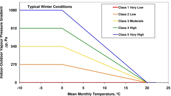
The Class model [10] is fairly straightforward. It assumes that the amount of atmospheric moisture indoors, expressed in terms of vapour pressure, is a function of the outdoor vapour pressure. Depending on the class of the building to be modeled a specified amount of internally generated moisture is added to the external vapour pressure. The amount of additional moisture load is modified according to the mean monthly ambient temperature, accounting for the effect of air changes. At colder temperatures the moisture surcharge is assumed to be at maximum while for warmer temperatures ventilation is assumed to remove most of the internally generated moisture. Between the two temperature thresholds linear interpolation is used to determine the moisture surcharge. The model is described below.

100 ) ( ) ( 100 ) ( ) ( sat e sat i i p p p p p ₌ +Δ = ϕ (%) Equation 1

The procedure defines five classes of buildings. The classes represent different levels of moisture generation rates related to the occupancy and use of the building. The classes are: Class 1, very low moisture generation; Class 2, low moisture generation; Class 3, moderate moisture generation; Class 4, high moisture generation; and Class 5, very high moisture generation.

More information on this model is given by Djebbar [12], Sandberg [13], and ISO [10]. The indoor/outdoor vapour pressure gradient Δp, can be determined from Figure 1.

0 270 540 810 1080 -10 -5 0 5 10 15 20 25

Mean Monthly Temperature, ºC

Indoor-Outdoor Vapour Pressure Gradient

Δ

p, Pa

Class 1 Very Low Class 2 Low Class 3 Moderate Class 4 High Class 5 Very High

Typical Winter Conditions

Figure 1 – Moisture surcharge to be added to external vapour pressure for predicting indoor RH.

BRE Model

The BRE Model is based on the mass difference between the moisture generation rate and the moisture gain or loss due to ventilation. Moisture absorption and desorption by interior finishes and furnishings are accounted for by a moisture admittance model. Jones [9] describes the BRE model. The indoor vapour pressure can be calculated using the following equation:

(

) (

[

)(

)

]

(

)

The ventilation rate can be calculated from:

v Q

I = total _{…Air changes/h Equation 3}

More information on this model is given by Jones [9], Christian [14], Djebbar [12], Loudon [15], El Diasty [16], and Oreszczyn [17].

ASHRAE 160P Method

ASHRAE Standard 160P, Design Criteria for Moisture Control in Buildings [11], is a proposed standard that specifies the criteria for performance-based design and mitigating moisture damage to the building envelope. Part of the standard specifies the criteria for inputs to various calculation procedures and simulation tools. The proposed standard has three procedures for calculating the indoor relative humidity, 1) the simplified method, 2) the intermediate method, and 3) the full parameter method, which is not addressed here. The simplified method is given below.

ϕi = 40% if To,daily <= -10°C

40% + (To,daily + 10) if -10°C< To,daily<20°C…(%) Equation 4

70% if To,daily => 20°C

The intermediate method is outlined below.

n ventilatio h o i Q m c p p • + = _,24 …(%) Equation 5

Design values for residential moisture generation •

m are based on the expected number of occupants. Design moisture generation rates are taken from ASHRAE 160P [11]. The ventilation rate can be determined from the air change rate.

3600 Iv Qventliation = …m 3 /s Equation 6 Field Measurements

In 2005 and 2006, surveys of indoor and outdoor conditions of relative humidity and temperature in twenty-four Canadian houses were carried out [5]. This activity was part of a project to develop durable, energy-efficient wall assemblies that can accommodate extreme outdoor and indoor climates in Canadian northern and northern coastal regions [18]. The surveys were carried to help in defining the effect of factors such as outdoor climate, occupant’s activities and house characteristics on the levels of indoor temperature and relative humidity. The data collected will be used for numerical modeling and laboratory studies to predict the hygrothermal response of promising wall assemblies. The three locations surveyed were Prince Rupert BC, Inuvik NT and Carmacks YT. Eight houses in each location were monitored. The houses were selected such that half the houses in each location had reported moisture problems. The houses surveyed did not feature designed mechanical ventilation, rather ventilation equipment was manually operated. Similarly since the sampling period was during the winter, cooling and dehumidification equipment if present was not operating.

For each of the twenty-four houses hand-size relative humidity and temperature sensors and data loggers were placed in two areas (usually a bathroom and another location) of the tenant living spaces for a month long period, capturing conditions every three minutes. Hourly averaged values for temperature and relative humidity were used for this analysis. One similar sensor was placed outside one of the houses in each region surveyed. The instruments were calibrated before being deployed and checked again after the survey program was completed. Information on the field measurements for the PERD-79 project can be found in Rousseau et. al. [5].

In Prince Rupert the survey sample included only two-storey row housing constructed in the 1980’s. The Prince Rupert house characteristics are given in Table 1. The Inuvik houses surveyed included a mix of row housing and fully detached houses. The homes were also a mix of single and two-storey homes constructed between 1975 and 1986. The Inuvik house characteristics are given in Table 2. In Carmacks survey sample included only one-storey single and fully detached houses, although one was a mobile home. Two of the homes were constructed in the late 1970’s. The remaining houses were constructed after 1995. The Carmacks house characteristics are given in Table 3.

A fourth set of interior temperature and relative humidity conditions was obtained from the Canadian Center for Housing Technology (CCHT) reference house, located in Ottawa ON [19]. CCHT features twin research houses to evaluate the whole-house performance of new technologies in side-by-side testing. Both houses are intensively monitored with simulated occupancy profiles. The CCHT reference house had a continuously operated mechanical ventilation system. The CCHT reference house characteristics are given in Table 4.

Modeling Assumptions

The following assumptions were made in applying the models tested: 1. The entire house volume is being modeled not the individual rooms.

2. The air change rate and or ventilation rates apply to the whole volume of house. As well the air leakage through the envelope is assumed to occur at a constant rate per area through the floor, exterior walls, and ceiling. The air change rate was based on the method given by ASHRAE [20].

3. The moisture generation rates are assumed to apply to the whole volume. 4. The interior temperature of the space is the temperature at sensor.

In order to use the BRE and ASHRAE 160P models it was necessary to estimate the hourly air change rate (ACH) or ventilation rate, Qtotal and Qventilation, for each of the

houses. The LBL model was used in this work, a simplified version of which is given in the ASHRAE Handbook of fundamentals [20]. The original model can be found in a paper by Sherman and Grimsrud [21]. For the surveyed houses the effective leakage area at 4 Pa, L, was derived from the results of blower fan door tests carried out on each house. The indoor temperature was assumed to be 21ºC while the outdoor temperature was the mean ambient temperature during the sampling period. The wind spend was taken to be the mean monthly wind speed. The house height was taken as the floor to ceiling height reported by the contractor. There was no information on the level of the neutral pressure plane; consequently the stack parameter was based on the ratios of the gross floor, ceiling, and exterior wall areas reported by the contractor assuming constant leakage through all the surface areas. A description of the model assumptions and error analysis is given by Cornick and Kumaran [22].

Sensitivity Analysis

Two models, the BRE and ASHRAE intermediate models, were investigated for sensitivity to input parameters. Parameters common to models, the ventilation rate (ACH) and the moisture generation rate were varied to examine the changes in MBE from the

measured results. As well for the BRE model the moisture admittance factors, α and β, were investigated

Results and Discussion

Overall Discussion

Overall the models examined have tendency to overestimate the indoor conditions except for the Class model, which for the houses surveyed over or underestimates depending on the house. Overall the ASHRAE intermediate model seemed to perform the best in terms of MBE, MAE, and RSME. Of the parameters used in this model the most sensitive parameter is the ventilation rate. Large changes occur over a small range of ventilation rates at the lower range (see Figure 2). Larger ventilation rates tend to bring the indoor air to outdoor conditions and the error trends towards a constant value with increasing ventilation rates. The ASHRAE intermediate model is less sensitive to changes in the moisture generation rates, especially at high ventilation rates.

The Class model performs surprisingly well for such a simple model. This was probably due to the fact that most houses monitored were close to the average house characteristics on which the Class model is based. The closer the house to the typical surveyed house the better the result, except for the CCHT reference house. The CCHT reference house was built to a high level of energy efficiency and consequently is very tight house from an air leakage perspective. This house is probably far from the typical house used in developing the Class model.

The BRE model generally overestimates and is clearly problematic. This can be seen by examining the formulation given in Equation 2. Suppose that the contribution from the exterior environment and the moisture generation were zero – the first and second terms in Equation 2. The last term represents the contribution of the interior surfaces and in this case is the only contributing factor to the interior RH. The values of α = 0.6 and β = 0.4 were suggested by Jones [9]. The range of calculated air change rates in the monitored houses was from 0.204 to 1.45. Thus the contribution of this term in the BRE model ranges from 0.50psat (50% RH) to 0.20 psat (20% RH). This represents a baseline relative humidity regardless of the contribution of the occupants or the exterior air. For the houses in Inuvik and the CCHT reference house this baseline RH was already above the measured RH. The BRE is sensitive to the β parameter, the desorption factor. Changes in this parameter, which is a function of the assumed RH at the desorbing surface can have large effects on the predicted RH, especially at lower ventilation rates. The model is less sensitive to the α parameter, the absorption factor, which tends to dampen the effect of ventilation air on the interior RH. Clearly the α, β coefficients are not appropriate for the majority of the North American houses monitored, as was noted by Jones [9]. The most sensitive parameter in the BRE model however is the ventilation rate. The effect of changes in ventilation rates is the same as the ASHRAE intermediate model (see Figure 2). The BRE model less sensitive to changes in the moisture generation rates.

-40.00 -20.00 0.00 20.00 40.00 60.00 80.00 100.00 0 1 2 3 4 5 6 7 8 9 10 11 12 13 14 15 1

Ventilation rate, air changes/h

M

ean bias error, %RH

6 BRE Model

ASHRAE Intermediate Model

Figure 2 – Sensitivity of the BRE and ASHRAE intermediate models to the ventilation rate

The ASHRAE simplified model is based on work conducted in Europe where it was considered to be within the recommended indoor humidity levels. This model was meant for design purposes and therefore overestimating the design loads is conservative. Comparing the ASHRAE simple model with measured results clearly indicates that it consistently overestimates the indoor RH. The model also fails to track well with exterior conditions that have an effect on the interior environment. The commentary in ASHRAE 160P states this clearly, “The simplified method may also produce high values for dry climates, even with air-conditioning. Again, the intermediate or full-parameter analysis would be preferable.” Given that ASHRAE simple model in many cases considerably overestimates the indoor RH it should only be used when no other information is available. It is not appropriate for use in cold climates where the 40% RH baseline is too high. Conservative loads estimates may preclude cheaper and more efficient designs. Generally the models track the indoor conditions except that the hourly variations are not captured. This is due to the fact that the moisture generation rates and ventilation rates are specified as average rates. A seemingly better trend is observed when twenty-four hour running averages for observed and predicted values are compared. In some circumstances this reduced the errors (MAE, MBE, and RMSE) but it did not change the overall bias of the models. A way of achieving better results would be to include variations in the moisture generation and air change rates. This however presumes that much more information is available, such as wind speed and direction as well as the occupant’s schedules and habits. This was not investigated.

Prince Rupert BC

The Prince Rupert climate is cool and wet. Of the 4 models tested the Class model showed the best concurrence generally showing the lowest MBE. The Class model, however, consistently underestimated the relative humidity in the space. The ASHRAE intermediate model also showed good concurrence but generally overestimated the relative humidity in the space. The BRE model showed large errors from the measured results and tends to overestimate, as did the ASHRAE simple model. House 5 was a typical example showing good concurrence for the Class and ASHRAE models. The results are shown in Figure 3. The error data are presented in the Appendix (See Table A 1).

Inuvik NT

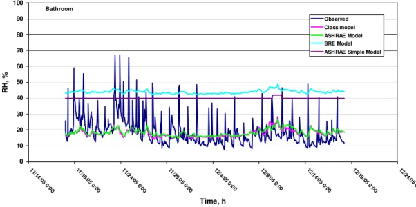
Inuvik is very cold and dry. The ASHRAE intermediate model showed the best concurrence generally showing the lowest MBE for the houses in Inuvik. The Class model also showed good concurrence but generally overestimated the relative humidity in the space. The BRE model showed large errors from the measured results and consistently overestimated, as did the ASHRAE simple model. The BRE and ASHRAE simple models have large systematic errors compared to the noise in the models while the ASHRAE intermediate and Class models show about the same amount of systematic error as the noise in the model. House 3 is a typical example showing good concurrence for the Class and ASHRAE intermediate models. The results are shown in Figure 4. The error data are presented in the Appendix (See Table A 2).

Carmacks YT

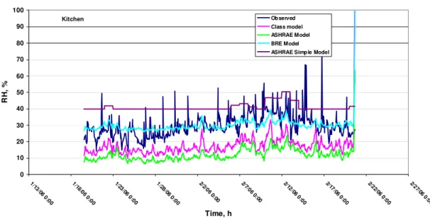
The Carmacks climate is very cold and dry. For Carmacks the Class model showed the best concurrence generally showing the lowest MBE. The Class model underestimated for the most part the relative humidity in the space, 9 of the 15 spaces. The BRE model also showed good concurrence but in most cases overestimated the relative humidity in the space depending on the house. The ASHRAE intermediate model sometimes showed large errors from the measured results and generally underestimates, as did the ASHRAE simple model. Like Inuvik the ASHRAE simple model showed a large systematic error. House 5 is a typical example showing, in this case, the best concurrence for the BRE model. The results are shown in Figure 5. The error data are presented in the Appendix (See Table A 3).

Ottawa ON

The Ottawa climate is cold and humid. Of the 4 models tested the ASHRAE intermediate model showed the best concurrence generally showing the lowest MBE. The Class model also showed good concurrence but overestimated the relative humidity in the space. The ASHRAE simple model showed a large error from the measured results and overestimated the RH. The BRE model also overestimated the relative humidity in the space and showed a large error performing worst of the four. The results are shown in Figure 6. The error data are presented in the Appendix (See Table A 4).

Conclusions

Four models, for predicting the indoor relative humidity in houses were tested against measured relative humidity data for 25 houses in Canada. The houses were typical of older North American construction methods. In assessing the models it should be noted that only 1 month of measured data used for comparison with predicted results. The month used was typical of the most extreme conditions occurring at the measurement sites. The models tested were the European Indoor Class Model, the BRE model, and the ASHRAE 160P simple and intermediate models. The RH in each house was measured in two different locations producing 50 different data sets. Hourly predictions were made using the four models and compared with the average hourly observations.

When compared with the measured data all the models generally overestimated the RH in the space. The ASHRAE intermediate model seemed to be the most robust exhibiting lowest Mean Bias, Mean Absolute, and Root Mean Squared Errors. The European Indoor Class also performed well for such a simple model and can be used when data regarding moisture generation and/or air change rates is not available. As a design tool however it should be noted that this model is not consistently conservative in predicting the indoor RH. The BRE is problematic and generally exhibits positive MBE’s as well large RMSE’s for the North American houses survey. This model should be used with caution as the α and β coefficients are probably not appropriate for the type of houses monitored, as was noted by Jones. The ASHRAE simple model exhibits large positive MBE’s and large RMSE’s as well. It does not trend well with measured data, especially when the interior conditions change with the exterior environment. This model was developed for design purposes and should be used as last resort even as a design tool. For colder climates overestimates of the design RH could lead to the unnecessary winnowing of cheaper more efficient designs. For models that use ventilation rates as a primary input it is imperative that these be determined accurately, as the models are very sensitive to changes in the ventilation rates especially at the lower range.

Acknowledgements

The authors would like to gratefully Ms. Marianne Manning for post-processing the raw monitoring data. Thanks are also extended to Ms. Madeleine Rousseau for organizing and managing the monitoring program and to Dr. Nady Saïd, investigator in the PERD 079 Project.

Table 1 – Physical characteristics of the eight houses surveyed in Prince Rupert BC.

Sensor Location a

Sensor Location b

Heating System Ventilation Class Volume m3 _{ACH @}

50 Pa Occupancy Moisture Generation Rate (ASHRAE 160P) L/day, Kg/day ACH (ASHRAE) Qventilation, m3/h α, β

House 1Main Floor Closet

Upstairs Bedroom Electric Baseboard

Kitchen - Manual, Bathroom - humidistat.

3 267 5.01 2 8 0.431 115.02 0.6, 0.4

House 2 Bathroom Main Floor

Storage

Hydronic Kitchen - Manual, Bathroom - humidistat.

3 244 7.35 3 12 0.649 158.25 0.6, 0.4 House 3 Bathroom Unknown Electric

Baseboard

Kitchen and Bathroom, manual

3 250 6.3 8 19 0.549 137.23 0.6, 0.4 House 4 Bathroom DHW Tank Room Electric

Baseboard

Kitchen - Manual, Bathroom - humidistat.

3 254 6.2 6 17 0.534 135.61 0.6, 0.4 House 5 Bathroom Main\Floor

Storage

Hydronic Kitchen - Manual, Bathroom - humidistat.

3 234 9.9 2 8 0.813 190.26 0.6, 0.4

House 6 Entrance Closet Bathroom Unknown Kitchen - Manual 3 210 6.36 3 12 0.548 115.16 0.6, 0.4

House 7 Bathroom Entrance Closet Electric Baseboard

Kitchen - Manual 3 251 5.3 4 14 0.459 115.25 0.6, 0.4 House 8 Coat Closet Bathroom Electric

Baseboard

Kitchen - Manual 3 225 6.7 2 8 0.509 114.60 0.6, 0.4

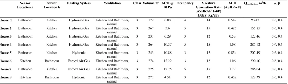
Table 2 – Physical characteristics of the eight houses surveyed in Inuvik NT.

Sensor Location a

Sensor Location b

Heating System Ventilation Class Volume m3 _{ACH @}

50 Pa Occupancy Moisture Generation Rate (ASHRAE 160P) L/day, Kg/day ACH (ASHRAE) Qventilation, m3/h α, β

House1 Bathroom Kitchen Hydronic/Gas Kitchen and Bathroom, manual

3 172 6.88 4 14 0.542 93.47 0.6, 0.4 House 2 Bathroom Kitchen Hydronic/Gas Kitchen and Bathroom,

manual

3 367 3.6 5 15 0.425 155.85 0.6, 0.4 House 3 Bathroom Kitchen Hydronic/Gas Kitchen and Bathroom,

manual

3 231 6.29 3 12 0.53 122.46 0.6, 0.4 House 4 Bathroom Kitchen Hydronic/Gas Kitchen and Bathroom,

manual

3 264 10.37 5 15 1.08 285.12 0.6, 0.4

House 5 Bathroom Kitchen Hydronic Kitchen and Bathroom,

manual

3 243 10.88 3 12 0.854 207.49 0.6, 0.4 House 6 Kitchen Bathroom Forced Air/Gas Kitchen and Bathroom,

manual

3 274 12.22 3 12 1.06 290.10 0.6, 0.4 House 7 Bathroom Kitchen Forced Air/Gas Kitchen and Bathroom,

manual

3 225 12.25 5 15 1.27 286.04 0.6, 0.4

House 8 Kitchen Bathroom Hydronic Kitchen and Bathroom,

manual

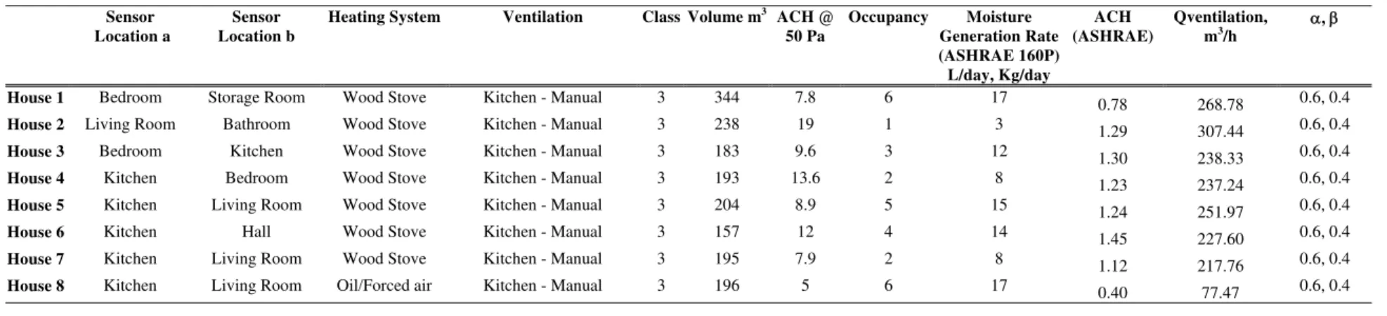
Table 3 – Physical characteristics of the eight houses surveyed in Carmacks YT.

Sensor Location a

Sensor Location b

Heating System Ventilation Class Volume m3 _{ACH @}

50 Pa Occupancy Moisture Generation Rate (ASHRAE 160P) L/day, Kg/day ACH (ASHRAE) Qventilation, m3_/h α, β

House 1 Bedroom Storage Room Wood Stove Kitchen - Manual 3 344 7.8 6 17 _{0.78 268.78} 0.6, 0.4

House 2 Living Room Bathroom Wood Stove Kitchen - Manual 3 238 19 1 3 _{1.29 307.44} 0.6, 0.4

House 3 Bedroom Kitchen Wood Stove Kitchen - Manual 3 183 9.6 3 12 _{1.30 238.33} 0.6, 0.4

House 4 Kitchen Bedroom Wood Stove Kitchen - Manual 3 193 13.6 2 8 _{1.23 237.24} 0.6, 0.4

House 5 Kitchen Living Room Wood Stove Kitchen - Manual 3 204 8.9 5 15 _{1.24 251.97} 0.6, 0.4

House 6 Kitchen Hall Wood Stove Kitchen - Manual 3 157 12 4 14 _{1.45 227.60} 0.6, 0.4

House 7 Kitchen Living Room Wood Stove Kitchen - Manual 3 195 7.9 2 8 _{1.12 217.76} 0.6, 0.4

House 8 Kitchen Living Room Oil/Forced air Kitchen - Manual 3 196 5 6 17 _{0.40 77.47} 0.6, 0.4

Table 4 – Physical characteristics of CCHT, Ottawa ON.

Sensor Location a

Sensor Location b

Heating System Ventilation Class Volume m3 _{ACH @}

50 Pa Occupancy Moisture Generation Rate (ASHRAE 160P) L/day, Kg/day ACH (ASHRAE) Qventilation, m3/h α, β

CCHT Main Floor Second Floor Gas/Forced air Heat recover ventilator @ 35 L/s supply

2 790 1.611 1* _{3 0.204 161.05 0.6, 0.4} * Humidity released from people not simulated during the period of the study.

Prince Rupert BC; House 5 0 10 20 30 40 50 60 70 80 90 100 4/₁₈ /05 0: 00 4/ 23/ 05 0 :0 0 4/ 28/ 05 0: 00 5/ 3/05 0: 00 5/_8/ 05 _0: 00 5/₁₃ /0 5 0: 00 5/₁₈ /05 0: 00 5/₂₃ /05 0: 00 5/₂₈ /05 0: 00 Time, h RH, % Observed Class model ASHRAE Model BRE Model ASHRAE Simple Model

Bathroom

Figure 3 – Comparison of the predictions of the four models with measured data over time for house number 5 in Prince Rupert BC. The sensor was located in the bathroom.

Inuvik NT; House 3 0 10 20 30 40 50 60 70 80 90 100 11 /14/ 05 0: 00 11 /19 /0_{5 0:} 00 11/ 24/₀₅ 0: 00 11/ 29/₀₅ 0 :0₀ 12 /4 /05 _0: 00 12 /9/_{05 0:} 00 12 /1_4/ 05 0: 00 12 /19/ 05 0: 00 12 /24/₀₅ 0 :00 Time, h RH , % Observed Class model ASHRAE Model BRE Model ASHRAE Simple Model

Bathroom

Figure 4 – Comparison of the predictions of the four models with measured data over time for house number 3 in Inuvik NT. The sensor was located in the bathroom.

Carmacks YT; House 5 0 10 20 30 40 50 60 70 80 90 100 1/ 13/ 06 _0: 00 1/ 18 /0_{6 0} :0₀ 1/23/ 06 0: 00 1/ 28/ 06 0: 00 2/_2/ 06 0 :0₀ 2/_7/ 06 0: 00 2/ 12/ 06 0: 00 2/₁₇ /06 0: 00 2/22 /06 0: 00 2/27 /06 0: 00 Time, h RH , % Observed Class model ASHRAE Model BRE Model ASHRAE Simple Model

Kitchen

Figure 5– Comparison of the predictions of the four models with measured data over time for house number 5 in Carmacks YT. The sensor was located in the kitchen.

Ottawa ON; CCHT 0 10 20 30 40 50 60 70 80 90 100 1/ 13 /06 0 :00 1/ 18 /06 0: 00 1/ 23 /06 0:₀₀ 1/ 28 /06 0:₀₀ 2/ 2/₀₆ 0: 00 2/ 7/_{06 0:0} 0 2/ 12 /06 0:₀₀ 2/ 17 /06 0:₀₀ 2/ 22 /0 6 0: 00 Time, h RH, % Observed Class model ASHRAE Model BRE Model ASHRAE Simple Model

Second Floor

Figure 6 – Comparison of the predictions of the four models with measured data over time for the CCHT reference house in Ottawa ON. The sensor was located on the second floor.

Appendix

Table A 1 – Errors from measured data from the Prince Rupert BC houses for the four different models tested.

Class Model

House House1 House2 House3 House4 House5 House6 House7 House8

Location a b a b a b a b a b a b a b a b MBE -8.94 -3.67 -6.94 -1.59 -7.87 -0.15 -8.12 0.11 -1.42 2.37 -6.91 -15.81 -12.86 -6.54 -4.37 -6.54 MAE 9.93 6.45 7.96 5.44 8.62 4.51 8.57 3.42 4.21 5.91 8.85 16.03 13.78 8.32 6.99 9.01 RSME 11.96 8.54 10.97 7.16 11.88 5.92 11.30 4.35 5.82 7.27 10.84 19.26 16.69 10.34 8.96 12.98 BRE Model MBE 9.20 12.50 11.22 14.32 16.36 24.61 15.85 23.57 13.22 14.18 13.60 1.98 9.82 16.49 15.47 11.80 MAE 9.42 12.59 12.25 14.32 17.32 24.61 16.14 23.57 13.43 14.18 13.77 6.27 11.22 16.49 15.49 13.87 RSME 10.87 13.59 13.48 15.04 18.53 25.02 17.37 24.03 14.50 14.86 15.57 7.93 12.73 17.26 16.20 14.89 ASHRAE Model MBE -0.81 5.24 1.85 8.68 15.01 21.45 10.18 19.32 0.44 4.65 8.60 2.83 6.17 12.12 2.74 1.17 MAE 5.80 7.10 6.45 9.20 16.27 21.46 11.15 19.32 4.54 5.91 9.88 9.30 10.40 12.60 6.05 7.38 RSME 7.29 8.45 8.25 10.37 18.16 22.62 12.53 19.89 6.01 7.02 11.99 11.21 13.13 14.88 7.19 10.09

ASHRAE Simple Model

MBE 13.22 14.56 18.27 17.37 14.71 24.59 17.91 24.40 27.33 23.94 15.11 -1.79 9.60 16.83 23.12 17.58 MAE 13.39 14.69 18.75 17.39 16.23 24.59 18.34 24.40 27.34 23.94 15.82 8.06 11.20 16.83 23.12 18.94

RSME 16.14 16.96 20.93 19.38 19.27 25.94 20.82 26.23 29.32 25.08 19.82 10.36 14.46 18.83 24.11 20.26

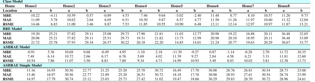
Table A 2 – Errors from measured data from the Inuvik NT houses for the four different models tested.

Class Model

House House1 House2 House3 House4 House5 House6 House7 House8

Location a b a b a b a b a b a b a b a b MBE -10.22 -4.11 10.59 0.57 -0.89 4.53 7.46 9.64 -5.02 -2.40 11.48 8.77 8.10 10.57 11.20 9.73 MAE 11.09 5.78 10.62 2.64 6.05 6.51 10.30 9.87 6.57 4.77 11.50 11.26 11.97 10.60 11.32 12.04 RSME 14.46 6.83 11.00 3.46 8.87 7.53 11.85 10.55 10.90 6.48 12.11 12.14 12.97 10.97 11.87 13.21 BRE Model MBE 19.20 25.21 37.82 29.11 25.08 29.73 17.90 21.81 11.03 12.77 20.98 19.22 16.88 20.11 36.48 32.65 MAE 20.08 25.21 37.82 29.11 25.51 29.73 19.31 21.82 13.73 12.99 20.98 20.10 18.95 20.11 36.48 33.09 RSME 21.72 25.78 37.93 29.34 26.57 30.22 20.18 22.20 14.85 14.01 21.24 20.77 19.63 20.29 36.67 33.77 ASHRAE Model MBE -0.91 5.36 10.68 0.68 -0.49 4.95 -1.10 2.18 -11.39 -9.27 0.87 -1.14 -0.28 2.70 11.72 10.35 MAE 7.48 6.14 10.72 2.66 6.17 6.76 5.69 4.02 11.39 9.27 2.84 4.58 6.21 3.31 11.81 12.60 RSME 10.54 7.86 11.07 3.50 8.83 7.80 9.34 4.71 14.99 10.93 3.49 8.03 10.02 3.81 12.38 13.73

ASHRAE Simple Model

MBE 11.16 16.95 30.56 22.77 21.25 25.20 25.70 30.72 16.49 17.70 30.08 28.76 26.81 30.54 28.73 23.08 MAE 13.46 16.97 30.56 22.77 21.89 25.20 26.51 30.72 18.18 17.76 30.08 28.93 27.61 30.54 28.74 23.99

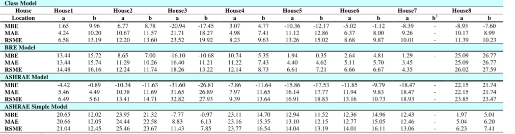
Table A 3 – Errors from measured data from the Carmacks YT houses for the four different models tested.

Class Model

House House1 House2 House3 House4 House5 House6 House7 House8

Location a b a b a b a b a b a b a b2 a b MBE 1.65 9.96 6.77 8.78 -20.94 -17.45 3.07 4.77 -10.36 -12.17 -5.02 -1.12 -8.39 - -8.93 -7.60 MAE 4.24 10.20 10.67 11.57 21.71 18.27 4.98 7.41 11.12 12.86 6.37 8.00 9.26 - 10.17 8.99 RSME 6.58 13.19 12.20 13.60 23.52 19.92 8.23 9.63 13.26 15.02 8.68 9.87 10.01 - 11.39 10.23 BRE Model MBE 13.44 15.72 8.65 7.00 -16.10 -10.68 10.74 5.35 1.94 0.35 2.64 4.81 1.29 - 25.09 26.77 MAE 13.44 15.74 11.29 10.26 16.40 11.21 11.22 7.43 4.40 4.62 5.11 5.70 3.45 25.09 26.77 RSME 14.48 16.16 12.24 11.74 18.26 13.22 12.14 8.73 6.61 7.21 6.66 6.67 4.35 26.02 27.59 ASHRAE Model MBE -4.42 -0.89 -10.34 -11.63 -31.60 -26.81 -7.86 -11.64 -15.86 -17.53 -11.85 -9.79 -18.47 - 22.15 21.74 MAE 5.46 4.49 10.38 11.69 31.65 26.89 7.97 11.65 16.14 17.77 11.94 9.83 18.47 - 22.15 21.74 RSME 6.49 5.61 13.41 14.71 32.82 27.93 9.39 13.64 16.91 18.83 13.16 10.73 18.93 - 23.85 23.47

ASHRAE Simple Model

MBE 20.65 12.02 23.95 21.32 -7.77 -0.97 23.11 14.70 12.94 11.52 12.36 14.96 12.43 - 1.97 5.01 MAE 20.66 12.05 24.44 22.58 8.83 6.13 23.16 15.35 13.10 12.15 12.77 15.05 12.46 - 5.04 6.20

RSME 21.04 12.45 25.46 23.67 11.43 7.85 23.77 16.54 14.04 13.19 14.01 16.11 13.06 - 6.23 7.41

2 – sensor malfunctioned

Table A 4 – Errors from measured data from the CCHT reference house in Ottawa ON for the four different models tested.

CCHT Reference House

Class Model BRE Model ASHRAE Model ASHRAE Simple

Model

Location a b a b a b a b

MBE 4.33 5.05 34.16 32.99 -1.59 -1.89 25.70 24.25

MAE 6.57 8.05 34.16 32.99 5.09 4.91 25.70 24.25

References

[1] Ojanen, T.; Kumaran, M.K. "Effect of exfiltration on the hygrothermal behaviour of a residential wall assembly," Journal of Thermal Insulation and Building

Envelopes, 19, pp. 215-227, January 01, 1996 (NRCC-39860).

[2] Ojanen, T.; Kumaran, M.K. "Effect of exfiltration on the hygrothermal behaviour of a residential wall assembly: Results from calculations and computer simulations," International Symposium on Moisture Problems in Building Walls (Porto,

Portugal, September 11, 1995), pp. 157-167, September 11, 1995 (NRCC-38783). [3] Ojanen, T.; Kumaran, M.K."Air exfiltration and moisture accumulation in residential

wall cavities," Thermal Performance of the Exteriour Envelopes of Buildings V : Proceedings of the ASHRAE/DOE/BTECC Conference (Clearwater Beach, FL., USA, December 07, 1992), pp. 491-500, 1992 (NRCC-33974) (IRC-P-1758). [4] Ojanen, T.; Kohonen, R.; Kumaran, M.K. "Modeling heat, air, and moisture transport

through building materials and components," Moisture Control in Buildings, ASTM Manual Series, MNL-18, Philadelphia, PA. : American Society for Testing and Materials, pp. 18-34, February 1994 (ISBN: 0803120561) (NRCC-37831) (IRC-P-3677).

[5] Rousseau, M., M. Manning, M.N. Said, S.M. Cornick, M.C. Swinton, and M.K. Kumaran “Characterization of Indoor Hygrothermal Conditions in Houses in Different Northern Climates”, Thermal Performance of the Exterior Envelopes of Whole Buildings X : Proceedings of the ASHRAE/DOE/BTECC Conference (Clearwater Beach, FL., USA, December 2-7, 2007).

[6] Tsuchiya, T. “Infiltration and indoor air temperatures and moisture variation in a detached residence,” J. the Soc. Heating, Air Cond., and San. Eng. of Japan, 54 No. 11, pp 13-19, 1980.

[7] Kusuda, T., “Indoor Humidty Calculations,”ASHRAE Trans. DC-83-12, No. 5, pp 728-740, 1983.

[8] Jones, R., Modelling water vapour conditions in buildings. Building Services Engineering Research and Technology, Vol. 14, No 3, pp 99-106, 1993. [9] Jones, R., Indoor Humidity Calculation Procedures Bldg. Serv. Eng. Res.

Technology, 16, No. 3, pp 119-126, 1995.

[10] International Standards Organization. ISO 13788:2001 (E). Hygrothermal performance of building components and building elements - Internal surface temperature to avoid critical surface humidity and interstitial condensation - Calculation method, 2001.

[11] ASHRAE SPC 160P, Working Draft Mar. 2006, pp. 6-7.

[12] Djebbar, R.; van Reenen, D.; Kumaran, M. K. "Indoor and outdoor weather analysis tool for hygrothermal modelling," 8th Conference on Building Science and Technology (Toronto, Ontario, 2/22/2001), pp. 139-157, May 01, 2001 (NRCC-44686) URL: http://irc.nrc-cnrc.gc.ca/fulltext/nrcc44686/

[13[ Sandberg, P.I., . Building components and building elements - calculation of surface temperature to avoid critical surface humidity and calculation of interstitial condensation. Draft European Standard CEN/TC 89/W 10 N 107, 1995

[15] Loudon, A. G., The effects of ventilation and building design factors on the risk of

condensation and mould growth in dwellings, Building Research Station Current Paper, 1971.

[16] El Diasty, R., P. Fazio and I. Budaiwi. Modelling of indoor air humidity: the

dynamic behaviour within an enclosure. Energy and Buildings, Vol. 19, pp.61-73, 1992.

[17] Oreszczyn, T. and S.E.C Pretlove. Condensation Targeter II: Modelling surface relative humidity to predict mould growth in dwellings. Proc. The Chartered Institution of Building Services Engineers: Building Services Engineering Research and Technology, Vol. 20, No 3, 1999.

[18] Saïd, M.N. "Building envelope researchers to develop wall assemblies suited to construction north of 60° " Construction Innovation, 10, (2), June, pp. 9, June 01, 2005. URL: http://irc.nrc-cnrc.gc.ca/pubs/ci/v10no2/v10no2_8_e.html

[19] Swinton, M.C.; Moussa, H.; Marchand, R.G. "Commissioning twin houses for assessing the performance of energy conserving technologies," Performance of Exterior Envelopes of Whole Buildings VIII Integration of Building Envelopes (Clearwater, Florida, December 02, 2001), pp. 1-10, December 07, 2001. (NRCC-44995) URL: http://irc.nrc-cnrc.gc.ca/pubs/fulltext/nrcc44995/

[20] ASHRAE, 2005 ASHRAE Handbook-Fundamentals. Atlanta, Ga.: American Society of Heating, Refrigerating and Air-Conditioning Engineers, Inc. Chapter 27.

[21] Sherman, M.H. and Grimsrud, D.T., 1980, “Infiltration-Pressurization Correlation: Simplified Physical Modeling,” ASHRAE Transactions, Vol. 86(2), pp. 778-803. [22] Cornick, S. M., and Kumaran M. K, “A Comparison of Measured Indoor Relative

Data with Results from Predictive Models,” IRC Research Report IRC-RR-231, June 2007.