Assessing Changeability in Aerospace Systems Architecting and Design Using Dynamic Multi-Attribute Tradespace Exploration

(1)

Assessing Changeability in Aerospace Systems Architecting

and Design Using Dynamic Multi-Attribute Tradespace

Exploration

Adam M Ross* and Daniel E. Hastings†

Massachusetts Institute of Technology, Cambridge, MA 02139, USA

A framework for assessing changeability in the context of dynamic Multi-Attribute Tradespace Exploration (MATE) is proposed and applied to three aerospace systems. The framework consists of two parts. First, changeability concepts such as flexibility, scalability, and robustness are defined in a value-centric context. These system properties are shown to relate “real-space to value-space” dynamic mappings to stakeholder-defined subjective “acceptable cost” thresholds. Second, network analysis is applied to a series of temporally linked tradespaces, allowing for the quantification of changeability as a decision metric for comparison across system architecture and design options. The quantifiable is defined as the filtered outdegree of each design node in a tradespace network formed by linking design options through explicitly defined prospective transition paths. Each of the system application studies are assessed in the two part framework and within each study, observations are made regarding the changeability of various design options. The three system applications include a hypothetical low Earth orbit satellite mission, a currently deployed weapon system, and a proposed large astronomical on-orbit observatory. Preliminary cross-application observations are made regarding the embedding of changeability into the system architecture or design. Results suggest that the low Earth orbit satellite mission can increase its changeability by having the ability to readily change its orbit. The weapon system can increase its changeability by continuing to embrace modularity, use of commercial off-the-shelf parts (COTS), and simple, excess capacity interfaces. The large astronomical observatory can increase its potential changeability by having the ability to reconfigure its physical payloads and reschedule its observing tasks. The analysis approach introduced in this paper is shown to be a powerful concept for focusing discussion, design, and assessment of the changeability of aerospace systems.

Topic Area: Space Systems – Systems Architecting, Systems Design, Changeability

Nomenclature

C = cost scalar

Ĉ = subjective cost threshold for change acceptability DVi = design variable element i, in general

DVi = specific design vector i

DV12 = design vector 1, variable element 2

{DVN} = design vector with N elements, in general fc = cost function, scalar function

fc({DVN}) = cost function, maps {DVN}ÆC

fc-1 = inverse cost function: ill-defined, Design Process

fU = utility function, scalar function

fU({XM}) = utility function, maps {XM}ÆU

FXM = attribute function, vector function. System Simulation

* Postdoctoral Associate, Engineering Systems Division, 77 Massachusetts Ave., Building 41-205, adamross@mit.edu, 617-253-7061, Member AIAA.

† Professor, Department of Aeronautics and Astronautics, and Engineering Systems Division, Fellow AIAA.

Space 2006

19 - 21 September 2006, San Jose, California

AIAA 2006-7255

(2)

FXM({DVN}) = attribute function, maps {DVN}Æ{XM}

FXM-1 = inverse attribute function, ill-defined, Goal Process

ki = multi-attribute utility function weight for attribute Xi

K = multi-attribute utility function normalization constant (not same as size({RK}) ) K = number of rules in rule set, (also different definition, see below

N = number of elements in design variable set, or vector

OD(<Ĉ,tˆ) = filtered outdegree (outdegree counting cost less than Ĉ and tˆ) Rk

= rule k Rk_(DV

iÆDVj) = rule k, connecting DVi to DVj

{RK} = rule set with K rules, in general

tˆ = subjective time threshold for change acceptability Tijk = transition matrix, elements “cost” of DViÆDVj using Rk

U = utility scalar, either single or multi-attribute derived Ui(Xi) = single attribute utility function on attribute Xi

U(X) = multi-attribute utility function, MAUF, on attribute set X X = attribute vector (same as set, {XM})

Xi = attribute element i, in general Xi = specific attribute set i

X12 = attribute set 1, attribute element 2

{XM} = attribute set with M elements, in general

I. Introduction

Developing complex aerospace systems requires architecting and design efforts maintain a delicate balance between providing often unique or novel benefits to demanding stakeholders, and keeping costs within reasonable bounds. Cost committal at the beginning of the architecting and design process makes early attention to design choices a high leverage point for improving system cost. Pressure to prematurely reduce a tradespace during Conceptual Design may inappropriately restrict design considerations, leading to less value-generating system choices. Multi-Attribute Tradespace Exploration (MATE) has proven to be a useful framework for capturing cost-benefit knowledge over a large tradespace, bringing to attention key trade-offs among requirements during early phases of design.1-4 Confounding traditional static approaches to design, however, is the existence of a dynamic system environment, both during development and operation. Ongoing MATE research has revealed a potential for using the framework to understand unarticulated value propositions arising from dynamic issues, including changing requirements (or preferences), incomplete information, and learning. Dynamic MATE analysis suggests that aerospace systems can be designed to continue to deliver value even when their context and stakeholder perspectives change.5

Space systems, in particular, face tremendous value disparities given the difficulty of physically altering space assets after launch, even though desires, expectations, and operating environments for the system may have changed during and after the system is developed and deployed. Repairing or otherwise altering assets on orbit can be construed in terms of ‘ease of change’ for the system (where the typical space system has relatively little “ease” of change). The changeability of the system directly relates to the time-varying ability of the system to deliver value (benefit at cost). Embedding, or at least assessing, the changeability of the system during early development stages will enable system architects and designers to positively influence the dynamic value of such systems. Part of the problem in focusing on changeability explicitly during design is the manifold ways in which it has been defined, either on its own or in terms of one of its many flavors including flexibility, adaptability, agility, extensibility, evolvability, among others.6-10 Fixing the definition of changeability in concrete, generalizeable terms will reduce ambiguity in communication and allow for its explicit consideration during design and decision making.

II. Defining Changeability

Change can be defined as the transition over time of a system to an altered state. If a system remains the same at time i and time i+1, then it has not changed. The inevitability of the effects of time on

State 2

State 1

“Cost” for change

Change agent

State 2

State 1

“Cost” for change

Change agent

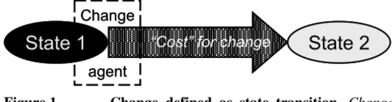
Figure 1. Change defined as state transition. Change specifications must include descriptions of beginning state 1, ending state 2, change mechanism including cost, and the change agent instigating the change.

(3)

systems and environments results in a constant stream of change, both of the system itself and of its environment. A change event can be viewed in three parts: the agent of change, the mechanism of change, and the effect of change. Fig. 1 displays these three parts. The agent of change is the instigator, or force, for the change. The role of change agent can be intentional or implied, but always requires the ability to set a change in motion. The mechanism of change describes the path taken in order to reach state 2 from state 1, including any costs, both time and money, incurred. The effect of change is the actual difference between the origin and destination states. A system that is black in time period one and gray in time period two has had its color changed. The change agent could be Nature, which can impart physical erosion due to wind, water, or sun, or could be a person with a paint can and brush. The change mechanism could be the erosion or painting process, costing no money, but taking a long time, or costing some amount of money, but taking a shorter amount of time.

When classifying a change on a system, the location for the change agent and the effect of the change must be explicitly considered. (The change mechanism “cost” will be discussed later.) A flexible change is a change instigated by a change agent external to the system boundary. An adaptable change is a change instigated by a change agent internal to the system boundary. When classifying the effects of change, the system can be parsed into design parameters and perceived value parameters, the latter sometimes referred to as “attributes.” The design parameters, sometimes referred to as “design variables,” are those aspects of a system design within the control of the system designer. The perceived value parameters are those aspects of a system design from which stakeholders derive value, often beyond the control of system designers.

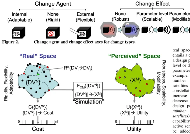
A value-centric change perspective will define changeability from the proper stakeholder perspective. The system designer may care about changes in design parameters, while customers, users, and other decision makers derive value from attributes, which can be on form or function of the system. A particular system design has a design parameter set and a value parameter, or attribute, set, the latter value-perceived by decision makers. A scalable change is a change in the level of a particular parameter. A modifiable change is a change in the parameter set of a system, including addition or subtraction. A robust system is one that is perceived to remain “constant” in spite of system external changes. Fig. 2 below shows the six change types grouped along two axes: change agent and change effect.

The change effect in a system can also be viewed along two axes: real space change and value space change. A

real space change entails a change in a design parameter level or the design parameter set. For example, the number of satellites in a constellation can increase or decrease (level in design parameter: number of satellites), or the capability for active sensing can be added to the previously passive payload of a

Change Agent

Internal (Adaptable) External (Flexible) None (Rigid)

Change Agent

Internal (Adaptable) External (Flexible) None (Rigid)

Change Effect

Parameter level (Scalable) Parameter set (Modifiable) None (Robust)

Change Effect

Figure 2. Change agent and change effect axes for change types.

RK_(DV iÆDVj)

{X

M

_}

U({XM_}) {XM_{}|Æ Utility} 0 1

Utility

0 1

Utility

“Perceived” Space

_Robust

n ess , Scalab ilit y, Modifi a bil ity

“Simulation”

F_XM({DVN_}) {DVN_}|Æ{XM_}

“Simulation”

F_XM({DVN_}) {DVN_}|Æ{XM_}

{DV

N

_}

C({DVN_}) {DVN_{} |Æ Cost}

“Real” Space

R igid ity , Fl exi bili ty , Adapt ab ilit y 0 Inf

Cost

0 Inf

Cost

Figure 3. Dynamic MATE variable mappings. Mappings show how changes in design space effect changes in value perception space.

(4)

satellite (addition of new design parameter: active sounding). A value space change entails a change in an attribute level or the attribute set. For example, suppose a decision maker cares about the following attributes: data latency, spatial resolution, and altitude. If a system changes from providing a data latency of 10 minutes to 5 minutes, or a spatial resolution of 1 m2 to 0.5 m2, that is a change in the level of an attribute (latency, and spatial resolution respectively). Adding the attribute data latitude diversity would be a change in attribute set. Scalability, modifiability, and robustness can apply to both design parameters and attributes.

Figure 3 shows the functional mapping of real space parameters to perceived, or value, space parameters. An aggregate measure of real space is the level of resources, or “cost,” required to create a system. Similarly, an aggregate measure of value space is the effective satisfaction, or “utility,” of a decision maker on the system. In the MATE process, system designers interview decision makers to determine value perceptions as reflected by attribute metrics, which are then aggregated by an elicited utility function. Designers then propose system concepts, parameterized by design parameters, in order to “perform” in the attributes. The “Simulation” is a set of models that determine how a particular design performs in the attributes, hence delivering a particular level of value, or utility, to a decision maker. Each particular design, likewise, requires expenditure of resources, or cost, in order to be created. Since flexibility and adaptability relate to the location of the change agent that instigates the actual change, it relates to the real space side. The attributes are in the minds of the value perceiving decision makers, so system designers must focus on how changes in design parameters map to changes in attributes. It is the changeability in the real space that will result in changeability in value space and thereby affect the dynamic value of a system.

Accounting for change must include specifications of change agent, change effect, and change mechanism. The first two were just described in terms of two change axes used to classify the change. The last part of change, change mechanism, plays a slightly different role. To describe a change, one must specify a beginning state, an ending state, and a transition path between the two. Observing a real world change scenario is an objective process: is the difference between the beginning and ending state nonzero? Assessing the acceptability of the change, however, is inherently subjective. For a system to follow a transition path from its beginning state to ending state necessitates the expenditure of resources (including time, knowledge, dollars, etc.). The acceptability of a given change to a decision maker is dependent on the availability of resources and the amenability of spending those resources. A one million dollar system modification may be acceptable to one decision maker, but not to another. In order to completely specify the changeability of a system, both the objective and subjective aspects of change must be considered and specified.

III. Quantifying Changeability

A reasonable approach to comparing a large number of systems simultaneously is through a tradespace. Fig. 4 below depicts the elements that go into tradespace development. Typically during concept exploration, a number of system designs and concepts are considered and assessed in terms of cost and benefit (i.e., value) to decision makers. The design parameters mentioned in the previous section represent the physical degrees of freedom for the system and can be assessed in terms of cost to develop through the mapping fC: {DVN}ÆC.

The attributes are a parameterization of value perceived by particular decision makers. Each decision maker specifies his or her own set with acceptable ranges, but whose specific values are derived from system designs being considered. The attributes can be aggregated in terms of value delivered to a decision maker through the concept of utility, with a function mapping fU:{XM}ÆU.

Each point is a specific design Attributes Utility Design Variables “Cost” Analysis

Tradespace: {Design,Attributes} ÅÆ {Cost,Utility}

Value Concept Firm Designer Customer User Each point is a specific design Attributes Utility Design Variables “Cost” Analysis

Tradespace: {Design,Attributes} ÅÆ {Cost,Utility}

Value Concept Firm Designer Customer User Each point is a specific design Attributes Utility Design Variables “Cost” Analysis

Tradespace: {Design,Attributes} ÅÆ {Cost,Utility}

Value Concept Firm Designer Customer User

Figure 4. Tradespace defined. Tradespaces are shorthand representations of designer controlled technical parameters and stakeholder perceived value parameters evaluated in terms of utility and cost (i.e., benefit and cost).

(5)

The typical tradespace plot displays the system designs on a Cost-Utility space, showing the resources required (cost) and value delivered (utility) for the systems in a concise format. A Pareto Set characterizes those designs of highest utility at a given cost, across all costs. This set often shows the tradeoff of cost incurred for increased value. Considering each design as a potential starting or ending state for change, the tradespace frame suggests a mechanism for considering the changeability of system designs. As mentioned in the previous section, change specification requires a beginning state, an ending state, and a transition path. If in addition to specifying design parameters (static representations of a system) designers specify transition paths (dynamic change opportunities), a traditional tradespace can become a tradespace network.

A network is a model representation of nodes and arcs. Each node represents a location, or state, with each arc representing a path that connects particular nodes. In a tradespace network, system designs are nodes and the transition paths are arcs. The transition paths represent each of the potential change mechanisms available to a particular design. Fig. 5 shows a traditional static utility-cost tradespace transformed into a tradespace network after the specification of transition rules, which are used to generate transition paths between design nodes. Transition rules, such as “burn on-board fuel to lower apogee” can be applied across a tradespace in an automated fashion to connect nodes efficiently. Designs that can follow more transition paths will have more outgoing arcs connecting it to other designs. In addition to representing an allowed transition, each arc has a cost associated with it, both in terms of dollars and time.

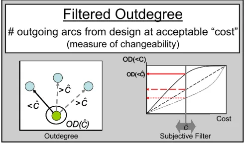
Each decision maker will have an acceptability threshold for time or money spent for enacting change. The number of outgoing arcs from a particular design is called the outdegree for that design. The number of outgoing arcs from a particular design whose cost is less than the acceptability threshold is called the filtered outdegree for that design. The filtered outdegree is a quantification of changeability for a design for a decision maker. (See Fig. 6 for a summary.) The higher the filtered outdegree of a design, the more changeable it is to that decision maker. The objective-subjective nature of the filtered outdegree captures the apparent relativity in perceived changeability of various designs: what may be flexible to one decision maker may not be flexible to another. The subjective acceptability threshold differentiates the results per decision maker. The objective outdegree calculation provides a mechanism for system designers to explicitly improve the potential changeability of a system: increase the number of outgoing arcs (add new transition rules), or reduce the cost of following outgoing arcs (increase the likelihood for arcs to cost less than acceptability threshold).

Filtered Outdegree

>

Cˆ OD(<C) C OD(< )Cˆ Cˆ OD(<C) C OD(< )Cˆ OD(< )Cˆ Cˆ OD(<C) C OD(< )Cˆ Cˆ OD(<C) C OD(< )Cˆ OD(< )Cˆ Cˆ Subjective Filter Outdegree Cost

Figure 6. Filtered outdegree defined. Filtered outdegree, a measure of changeability, counts the number of potential transition paths available to a design, filtered by acceptable cost for change by a particular decision maker.

Cost

Utility

Cost

Utility

Cost

Utility

Cost

Utility

Transition rules

Figure 5. Tradespace network. Specifying transition rules transforms a tradespace into a tradespace network, with transitionable designs accessible through heterogeneous arcs for each rule.

(6)

IV. Case Applications

A number of case applications were conducted to validate the prior proposed quantification of changeability. For each case, design parameters, attributes, and transition rules were proposed. Models were developed to determine the attribute values for particular designs, cost models were developed to determine the cost for particular design parameter set values, and utility models were developed to determine the value perceived for particular attribute set values.

A. Hypothetical Low Earth orbit Satellite Mission

The first case application is to a hypothetical low Earth orbit satellite mission called X-TOS, Terrestrial Observer Satellite X, whose goal is to study atmospheric density using an in-situ payload. The system design and models were developed by a graduate space system design course at the Massachusetts Institute of Technology in the spring of

2002. The key system decision maker was a payload scientist from Hanscom Air Force Research Laboratory. The design team proposed numerous concepts for achieving the mission and eventually settled upon the design parameters listed in Table 1.11

The design parameters given in Table 1 were varied, or enumerated, to produce 7840 combinations of values corresponding to unique design options to be considered. These design options were then evaluated in terms of cost to develop and performance in terms of the attributes listed in Table 1. (The “Current” indication means that the parameter is presently considered by the designer or decision maker. An alternate value of “Potential” refers to possible future consideration.) The attribute values were then passed through a multi-attribute utility function to aggregate the perceived value of each design to the “Science” decision maker. The utility function can take on a value between zero (minimally acceptable) and one (ideal). If any attribute value for a given design option is outside the acceptable range for the decision maker, the utility value for that design is undefined and the design option is deemed unacceptable. 3384 out of the 7840 combinations resulted in valid (acceptable) design options. Fig. 7 depicts the original static tradespace results for the X-TOS designs being considered. The “best” design options are those at highest utility at a given cost.

The next step in dynamic MATE analysis is to move from a static to a dynamic perspective. If a designer or decision maker were to change his mind during development or after deployment, dynamic analysis would help to anticipate how the current accepted design could be changed into a new one.

1. Transition rules

Table 1. X-TOS design parameters and attributes.

Design Parameters Attributes

Inclination Inc Current Data Lifespan DL Current

Apogee Altitude Aa Current Latitude Diversity LD Current

Perigee Altitude Ap Current Equator Time ET Current

Communication Architecture CA Current Latency L Current

Total Delta-V ∆V Current Sample Altitude SA Current

Propulsion Type PpT Current

Power Type PwT Current

Antenna Gain AG Current

(7)

Transition rules were developed based on the

design parameters investigated. Mechanisms to

“get there from here” included creative approaches to altering design parameter values, both by trading one value for another (internally motivated, or adaptable-type, change) and through influence of outside intervention (externally motivated, or flexible-type, change). Table 2 lists eight proposed transition rules and Fig. 8 shows the effect of the rules on design variables. The arrow direction in the figure indicates the effect of a given rule on a given design parameter (increase, decrease, or either). Path enablers are intervening parameters that reduce the cost for transition paths for a design, including creation of the path option itself. The path enablers considered for X-TOS were refuelability, tugability, and upgradeability. These three enablers were considered binary in that if they existed, the paths were allowed. The green ‘X’ in the cells below Path Enablers in Fig. 8 means that those enablers are required in order for that change effect to be possible. The Change Origin indication keeps track of whether the rule is perceived to be motivated external to the system boundary (‘Flx’=Flexible-type change) or internal to the system boundary (‘Adp’=Adaptable-type change).

2. Changeability assessment

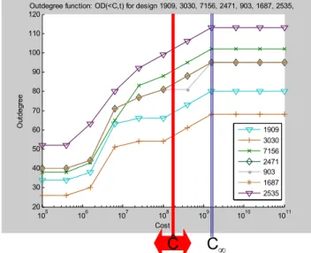
Once the transition rules were developed, a computer algorithm determined which designs were accessible from any given design using any particular rule. For the case study, the static tradespace included 3384 distinct design parameter set enumerations and their corresponding attribute values. Given eight transition rules, the potential number of arcs is approximately 8×33842. Once allowed arcs were determined, the tradespace network was analyzed to determine each design’s outdegree. Since the perceived changeability of a design includes the subjective acceptability threshold, for each design, the outdegree must be filtered by only counting outgoing arcs with acceptable cost. In order to better understand the function of outdegree versus acceptability threshold, the filtered outdegree function, OD(<C,t), can be generated by varying the cost threshold and determining the outdegree for that particular threshold. An example of the X-TOS OD(<C,t) function is given in Fig. 9. Seven designs are plotted,

Rule-Effects Matrix

X-TOS Inc Aa Ap CA ∆V PpT PwT AG Rf Tg Up DV1 DV2 DV3 DV4 DV5 DV6 DV7 DV8 IV1 IV2 IV3 Flx Adp Rule Plane change R1

Apogee burn R2 Perigee burn R3 Plane tug R4 Apogee tug R5 Perigee tug R6 Space refuel R7 Add sat R8 Origin Design Variables Path Enablers Change

Figure 8. X-TOS Rule-Effects Matrix. Lists both actual and potential rules for analysis, requirements for enabling variables, and change type by origin. 105 106 107 108 109 1010 1011 20 30 40 50 60 70 80 90 100 110

120Outdegree function: OD(<C,t) for design 1909, 3030, 7156, 2471, 903, 1687, 2535,

Cost Ou td eg re e 1909 3030 7156 2471 903 1687 2535

Ĉ

C

_∞

Figure 9. X-TOS Outdegree Function, OD(<C,t). Table 2. X-TOS transition rules.

Rule Description Change agent origin

R1: Plane Change Increase/decrease inclination, decrease ∆V Internal (Adaptable) R2: Apogee Burn Increase/decrease apogee, decrease ∆V Internal (Adaptable) R3: Perigee Burn Increase/decrease perigee, decrease ∆V Internal (Adaptable) R4: Plane Tug Increase/decrease inclination, requires “tugable” External (Flexible) R5: Apogee Tug Increase/decrease apogee, requires “tugable” External (Flexible) R6: Perigee Tug Increase/decrease perigee, requires “tugable” External (Flexible) R7: Space Refuel Increase ∆V, requires “refuelable” External (Flexible) R8: Add Sat Change all orbit, ∆V External (Flexible)

(8)

showing their filtered outdegree as a function of cost threshold. As the cost threshold increases, the outdegree increases, to a point. The cost above which no outdegree increase occurs is C∞, and represents the point at which all paths are counted and no new transition mechanisms are enabled. Notice that design 7156 changes from being the third least changeable to the second most changeable design as the cost threshold increases. The maximum changeability for a system occurs when the decision maker’s cost threshold is above C∞. Fig. 10 lists the design parameter values for the Fig. 9 X-TOS designs.

Figure 11 depicts the outdegree tradespace showing design number versus outdegree as colored by cost threshold. (The scale on the right shows increasing acceptable cost threshold for smaller circles.) As the cost threshold increases, the outdegree of the designs increase differentially. For example, design number 2600 has a smaller outdegree than design number 3050 at a cost threshold of 4×105, but that same design has a larger outdegree than design 3050 when the cost threshold is increased to 2.5×1010. The differential nature of the outdegree function shows that designs perceived as most

4.21 150 2.27 6 140 0.51 Low Fuel Cell Chem 1200 TDRSS 150 460 70 1687 4.21 150 2.27 11 60 0.51 Low Fuel Cell Chem 1200 TDRSS 150 460 30 903 4.21 150 2.27 5 180 0.51 Low Fuel Cell Chem 1200 TDRSS 150 460 90 2471 4.15 4.99 4.52 4.88 Cost ($10M) 350 150 150 290 Sample Alt 2.40 2.67 2.42 2.30 Latency 5 2 2 5 Eq Time 180 180 140 180 Lat Div 11 0.61 0.52 10.05 Data Life Low Low Low Low Ant Gain Solar Array Solar Array Fuel Cell Fuel Cell Pwr Type Chem Elec Elec Chem Prop Type 1000 1200 1200 1200 Delta V TDRSS TDRSS TDRSS TDRSS Com Arch 350 150 150 290 Perigee 770 2000 1075 460 Apogee 90 90 70 90 Inclination 7156 3030 1909 2535 DV 4.21 150 2.27 6 140 0.51 Low Fuel Cell Chem 1200 TDRSS 150 460 70 1687 4.21 150 2.27 11 60 0.51 Low Fuel Cell Chem 1200 TDRSS 150 460 30 903 4.21 150 2.27 5 180 0.51 Low Fuel Cell Chem 1200 TDRSS 150 460 90 2471 4.15 4.99 4.52 4.88 Cost ($10M) 350 150 150 290 Sample Alt 2.40 2.67 2.42 2.30 Latency 5 2 2 5 Eq Time 180 180 140 180 Lat Div 11 0.61 0.52 10.05 Data Life Low Low Low Low Ant Gain Solar Array Solar Array Fuel Cell Fuel Cell Pwr Type Chem Elec Elec Chem Prop Type 1000 1200 1200 1200 Delta V TDRSS TDRSS TDRSS TDRSS Com Arch 350 150 150 290 Perigee 770 2000 1075 460 Apogee 90 90 70 90 Inclination 7156 3030 1909 2535 DV

Figure 10. Design variable values for designs in Fig. 9.

Figure 11. X-TOS outdegree tradespace of outdegree versus design ID number.

For this plot, Ĉ=C_∞

More changeable

(ie including flexible, adaptable, scalable

and modifiable)

Colored by outdegree

(9)

changeable will vary depending on the subjective cost threshold (what is changeable to decision maker A may not be changeable to decision maker B, even if they have the same attribute set and utility curves). Understanding the shape of a design’s outdegree function can enable a designer to aim for the “sweet spot” of a design to increase a system’s perceived changeability. For a given cost threshold, a traditional tradespace plot can be shown, colored by outdegree, depicting the utility-cost location of the most changeable designs. Fig. 12 shows the X-TOS tradespace colored by outdegree when the cost threshold is greater than C∞. In this colored tradespace, it is apparent that the Pareto Set designs are not necessarily the most changeable. If requirements or value perceptions change, the current best designs may rapidly lose their optimal status. Changeable designs may have the advantage in such a context, being able to more easily move to higher value regions in the new context-defined tradespace.

3. Insights

While the X-TOS mission was mostly theoretical in nature, the analysis exercise is nonetheless instructive. Through specification of transition rules, enumeration of the tradespace network was readily automated, though time-consuming. (The algorithm ran in approximately 12 hours, determining if rule k linked node i to node j, for k=1 to 8, i,j ∈ tradespace of size N=3384.) Calculation of the filtered outdegree requires explicit conversations with decision makers to determine their acceptable cost threshold for changeability. Absent the threshold knowledge, the outdegree functions for each design can be determined objectively. Determining the most “changeable,” or “flexible” designs requires knowledge of the acceptable cost threshold. Quantification of changeability at a particular cost threshold does allow for explicit consideration of changeability, as shown through the colored tradespace plots in Fig. 12. If designers explicitly consider transition rules during design, the changeability of design options will necessarily increase over the ad hoc considerations that may be currently at work. Embracing path enablers, such as on-board refueling or grapple points for tugging, increases changeability for X-TOS-like systems, particularly those missions driven by orbit parameters.

B. Currently Deployed Weapon System

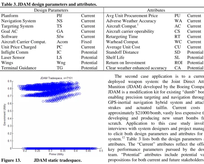
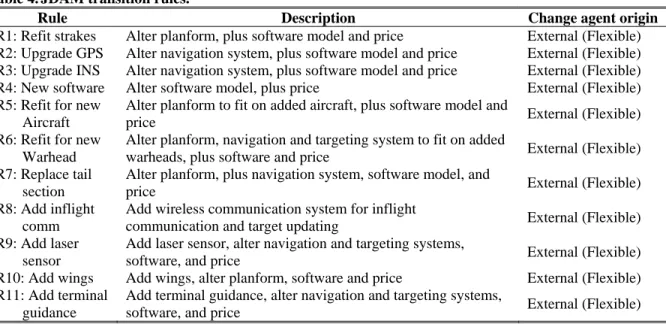
The second case application is to a currently deployed weapon system: the Joint Direct Attack Munition (JDAM) developed by the Boeing Company. JDAM is a modification kit for existing “dumb” bombs enabling precision targeting and navigation through a GPS-inertial navigation hybrid system and attached strakes and actuated tailfin. Current costs are approximately $21000/bomb, vastly less expensive than developing and producing new smart bombs from scratch. Application to this case study involved interviews with system designers and project managers to elicit both design parameters and attributes for the system.12 Table 3 lists both the design parameters and attributes. The “Current” attributes reflect the official key performance parameters pursued by the design team. “Potential” attributes include potential value propositions for both current and future stakeholders for Table 3. JDAM design parameters and attributes.

Planform Plf Current Avg Unit Procurement Price PU Current Navigation System NS Current Adverse Weather Accuracy WA Current

Targeting System TS Current Aircraft Compat.1 AC Current

Goal AC GA Current Aircraft carrier operability CS Current

Software Sfw Current Retargeting Time RT Current

Aircraft Carrier Compat. Acom Fixed Warhead Compat. WC Current

Unit Price Charged PC Current Average Unit Cost CU Current

Inflight Comm IC Potential Standoff Distance SD Potential

Laser Sensor LS Potential Shelf Life SL Potential

Wings Wng Potential Return on Investment ROI Potential

Terminal Guidance TG Potential Clear weather enhanced accuracy CA Potential

(10)

the system as brainstormed through future scenario considerations. “Fixed” design parameters were not varied for the study, but instead were used as hard constraints. A relatively simple system model was developed using basic physics and control loops. 7151 enumerations of the design parameters were evaluated with the model in terms of attributes and cost. The attributes were run through two utility functions: one for the “Government” decision maker, representing the acquiring agency, and one for the “Prime” decision maker, representing the system development organization. Fig. 13 shows the JDAM tradespace in terms of utility to the two decision makers. “Best” design options are at highest utility for a fixed other utility (top right corner in the plot). The row of zero government utility options represent the “dumb” bomb enumerations that would still provide value to the Prime decision maker, but not to the Government decision maker. (In general a zero utility represents the minimally acceptable value, but for illustrative purposes, designs with undefined utility were rounded up to zero to show the large number of potentially unacceptable designs.)

The transition rules proposed for JDAM case study are listed in Table 4. The rules were developed in order to alter the design parameter set, both in terms of values of particular parameters and in terms of adding new parameters to the set (allowing for the enumeration of future system variants). Unlike the X-TOS rules, all of these rules were externally motivated (flexible-type changes) due to an inability to conceive of mechanisms paying down one design parameter in order to gain another. Fig. 14 lists the rules and their effects on the design parameters, including the cases where the presence of path enablers may lower the cost for paths. Yellow diagonal marks in the Path Enabler columns represent their optional nature. The two path enablers considered in this case study were Modularity and COTS parts, representing design philosophies for architecture and Figure 14. JDAM Rule-Effects Matrix.

Table 4. JDAM transition rules.

R1: Refit strakes Alter planform, plus software model and price External (Flexible) R2: Upgrade GPS Alter navigation system, plus software model and price External (Flexible) R3: Upgrade INS Alter navigation system, plus software model and price External (Flexible) R4: New software Alter software model, plus price External (Flexible) R5: Refit for new

Aircraft

Alter planform to fit on added aircraft, plus software model and

price External (Flexible)

R6: Refit for new Warhead

Alter planform, navigation and targeting system to fit on added

warheads, plus software and price External (Flexible) R7: Replace tail

section

Alter planform, plus navigation system, software model, and

price External (Flexible)

R8: Add inflight comm

Add wireless communication system for inflight

communication and target updating External (Flexible) R9: Add laser

sensor

Add laser sensor, alter navigation and targeting systems,

software, and price External (Flexible)

R10: Add wings Add wings, alter planform, software and price External (Flexible) R11: Add terminal

guidance

Add terminal guidance, alter navigation and targeting systems,

(11)

component selection respectively. 2. Changeability assessment

Implementation of the transition rules proposed in Table 4 requires adequate modeling of the system to understand path costs and times. Due to low system model fidelity, a changeability model of appropriate fidelity should be used. Qualitatively, the changeability analysis needs to address whether a specific design can follow a given transition rule and at what cost and time. More changeable designs will have a higher outdegree than less changeable designs.

Since the models used are not accurate enough to perform detailed quantitative tradespace network analysis, instead a semi-quantitative approach can be used to assess the changeability of the JDAM designs.

The designs to consider for the changeability assessment will be the eight designs from the Pareto Set, recaptured in Fig 15 and Fig. 16 (The Pareto Set is the set of designs that have highest utility at a given cost summed across all costs.)

A simplification to replace calculation of the full tradespace network outdegree for each design is to assess the number of rules that can be followed from a particular design. Given a cost threshold for acceptability, the number of accessible rules will reflect the changeability of each design. Supposing cost and time can be categorized as “low,” “medium,” and “high,” the eight designs can be assessed in terms of how much each rule “costs” for dollars and time.

Figure 17 captures the qualitative assessment of costs in terms of dollars and time for following each rule for each of the Pareto Set designs. The maximum rule outdegree, or MaxOD, is the total number of rules: in this case 11. The filter is set at a “Medium” dollar cost and a “Medium” time cost; only paths that cost “M” or less will be counted towards the outdegree. The red bars indicate rules that cannot be followed given the subjective threshold. (The outdegree function can be None None None None None None None None TG .894 .885 .880 .875 .863 .823 .810 .732 U_DM1 .376 .384 .402 .406 .409 .411 .415 .416 U_DM2 None None None None None None None None Wng None None None None None None None None LS 18K 18K 16K 16K 16K 16K 16K 16K PU Med Simple Simple Simple Simple Simple Simple Simple Sfw All All All All All All All All GA Far comm Far comm Far comm Far comm Far comm Static data Static data Static data TS INS/ GPS+/ ACup INS/ GPS+/ ACup INS/ GPS/A Cup INS/ GPS GPS only INS/ GPS GPS only INS only NS Strake/ Fin Strake/ Fin Strake/ Fin Strake/ Fin Strake/ Fin Strake/ Fin Strake/ Fin Strake/ Fin Plf 8 7 6 5 4 3 2 1 None None None None None None None None TG .894 .885 .880 .875 .863 .823 .810 .732 U_DM1 .376 .384 .402 .406 .409 .411 .415 .416 U_DM2 None None None None None None None None Wng None None None None None None None None LS 18K 18K 16K 16K 16K 16K 16K 16K PU Med Simple Simple Simple Simple Simple Simple Simple Sfw All All All All All All All All GA Far comm Far comm Far comm Far comm Far comm Static data Static data Static data TS INS/ GPS+/ ACup INS/ GPS+/ ACup INS/ GPS/A Cup INS/ GPS GPS only INS/ GPS GPS only INS only NS Strake/ Fin Strake/ Fin Strake/ Fin Strake/ Fin Strake/ Fin Strake/ Fin Strake/ Fin Strake/ Fin Plf 8 7 6 5 4 3 2 1

Figure 15. JDAM Pareto Set designs.

Figure 17. Qualitative changeability assessment for JDAM Pareto Set designs. 1 2 34 5 6 7 8 1 2 34 5 6 7 8

(12)

derived by varying the

Ĉ and tˆ cost

thresholds and calculating the resulting outdegree. It is apparent that the changeability of each design is subjectively affected by how much a decision maker is willing to “spend” to get the desired change.) The results in this figure are more qualitative than detailed network modeling would provide, but still instructive. The following figures will consider the effect of adding the path enablers Modularity and COTS to the designs. These path

enablers will differentially affect the

“cost” to follow each rule for each design option. The outdegree assessment done here can be used as a filter for refining system designs at the more detailed level. Additional path enablers could be proposed at this stage as the changeability becomes a more central consideration of the analysis. Figure 18 shows the outdegree assessment with the

inclusion of Modularity into the

designs. The effect is predominantly a decrease in transition time for several, but not all of the rules. For the case studied here, none of the filtered ODs are changed over the non-modularity Figure 18. Qualitative changeability assessment for JDAM Pareto Set designs,

including Modularity path enabler.

Figure 20. Qualitative changeability assessment for JDAM Pareto Set designs, including Modularity and COTS path enablers (and showing JDAM2=real design). Figure 19 Qualitative changeability assessment for JDAM Pareto Set designs, including COTS path enabler.

(13)

cases, suggesting it does not increase the subjective changeability of the system. Fig. 19 shows the outdegree assessment with the inclusion of COTS into the designs. The effect is predominantly a decrease in dollar cost for several, but not all of the rules. For the case studied here, all of the designs see an increase in apparent changeability. Fig. 20 shows the outdegree assessment with the inclusion of both Modularity and COTS into the designs. Since these path enablers tend to work on different “costs” they work synergistically to increase the changeability across the designs, in particular raising the changeability of the least changeable designs from the first assessment. The actual fielded JDAM system is added to this last figure for comparison.

The actual JDAM system did in fact incorporate several path enabling aspects. According to the person in charge of the original JDAM airframe design, and current JDAM “accessory” manager, the system embraced the following three concepts: use of modularity, use of commercial off the shelf (COTS) parts, and the use of simple interfaces with excess capacity. The first path enabler, modularity, while not in use throughout the system, was used when possible in order to isolate the system from component changes and to speed up assembly time of the system in the field. Modularity also gave the system the ability to be readily upgraded. The tail fin section has three motors, each controlling a single fin. The motor assembly was designed as a module for simple insertion into the system. For all JDAM variants, except for one, the motor module is the same. The exception is the smallest variant of JDAM, whose tail section is too small to house a modular motor. The “cost” of modularity for the motor is a larger size, which cannot be accommodated by the smaller tail section on the JDAM variant for the Mark-82 warhead.

In order to reduce cost, the team embraced the second path enabler, a COTS philosophy, seeking an already developed commercial alternative to a higher grade military-spec hardware. The commercial components had to meet stringent reliability and performance measures, but were hands down less expensive than custom hardware. (In fact, approximately 30% of the cost savings for the system resulted from using lower cost materials and parts.)13 Using COTS extended to JDAM “accessories,” or upgrades, will reduce the cost of changing the system.

The third path enabler was simple, excess capacity interfaces. A single 1760 standard interface provided connectivity to the aircraft carrying the JDAM. Extra pins in the connector were provided in order to have extra capacity. The designers could have reduced cost by having fewer pins and smaller cables, but felt that the system should have extra capacity “in case of future needs.” Another example is in the selection of GPS receiver. The GPS receiver is plugged into the Guidance Control Unit, or the “brain” of the bomb. The interface to the GPS receiver was designed to have 12 channels, even though the original receiver had only 5 channels and the software could not yet handle additional channels. When newer GPS receivers were later developed, it could be easily installed into the JDAM, with the software upgrades happening even later.

These three path enablers result in the ability to alter the JDAM system at relatively low cost and time. The generic nature of the interface standard does not over restrict the possibilities for add-ons either, thereby increasing the number of “paths” from the current system.

3. Insights

An open question is whether JDAM is an exceptional case in aerospace system development. Its special status as a test program for acquisition reform freed the team from the burden of paperwork and constraints on design.14 Class 2 change authority and ownership of the design specifications gave the Prime both power to make value-adding decisions, and the incentive to produce a high quality product. The retention of ownership, in particular, enabled the Prime to take on the cost burden of building in path enablers. In general, if a decision maker does not articulate the desire for changeability, he will be unwilling to pay for it since it may represent unused functionality. In the case of JDAM, the Prime “paid” for the unused functionality by anticipating the need to change. In effect, JDAM reduced its time constant for change by having the path enablers. The Prime must have decided that the cost of “carrying” the path enablers was lower over the long run than developing a new system when the demand for change arrived from the customer.

JDAM has been widely perceived to be a successful and flexible system. The analysis in this case confirms that perception. The presence of several path enablers reduces the “cost” and increases the number of change possibilities for the system. Modularity reduces the time for change, while COTS reduces the cost for change. The simple, excess capacity interfaces increases the potential change types for the system.

(14)

The third case application is to a proposed large astronomical on-orbit observatory, the Terrestrial Planet Finder (TPF) mission being developed by the Jet Propulsion Laboratory (JPL). The TPF mission is to discover whether life exists on other worlds through the discovery of Earth-like planets in the habitable zones around distant stars. Concepts currently being considered include an infrared interferometer and visible coronagraph. The former requires a set of smaller individual telescopes that cooperatively observe stellar light and recombine the observations to simulate a larger aperture telescope. The design parameters and attributes for the case application are listed in Table 6. The design parameters were developed by Brian Makins as part of his Master of Science thesis at MIT, and reflect the major design “knobs” for an interferometer-class on-orbit observatory.15 The attributes are derived from the TPF Science Working Group (SWG) mission goals as interpreted by Makins, representing the “Science” decision maker. “Current” attributes include those explicitly defined by the TPF SWG, while the “Potential” attributes include those proposed by Makins. The performance and cost models used, the TPF Mission Analysis Software (TMAS), were developed by the MIT Space System Laboratory (SSL) and refined by Makins. Fig. 21 shows the static TPF tradespace for the 10611 design parameter set enumerations considered. The zero “Science” utility points in the figure are those designs that fail to meet the mission requirements. (Usually zero utility corresponds to the set of minimally acceptable designs, but in this case were included to show the large number of unacceptable designs.)

The transition rules for TPF are listed in Table 7. Depending on the definition for the system boundary, the rules could be classified as either internal (adaptable-type change) or external (flexible-type change). For the purposes of this case, the ground operations center was Figure 22. Proposed TPF transition rules.

Table 6. TPF Design Parameters and Attributes.

Orbit Type OT Current Number of Surveys S Current

Num Apertures NA Current Num Medium Spectroscopies MS Current

Wavelength Wl Current Num Deep Spectroscopies DS Current

Interferometer Type IT Current Number of Images1 I Current

Aperture Type AT Current Num Long Baseline images IL Potential Aspect Ratio AR Current Num Short Baseline images IS Potential

Aperture Size AS Current Annual Ops Cost Ops Potential

Interferometer Baseline IB Current

Schedule Sc Potential

Design Lifetime DL Fixed

Table 7. TPF transition rules.

R1: Change baseline Expand or contract baseline Internal (adaptable) R2: Increase NA Add to number of apertures External (flexible) R3: Change schedule Alter observation schedule External (flexible) R4: Extend life Add time to active mission duration External (flexible) Figure 21. TPF static tradespace.

(15)

considered to be external to the system boundary, so changes in observation schedule are seen to be instigated by a change agent external to the system, and hence a flexible-type change. Several possible change rules are mentioned in Table 7 and restated in Fig 22 showing their effects on design parameters. In particular, changing baseline and increasing the number of apertures allows for scalability of mission attribute performance (an increase in the rate and sensitivity of observation modes). In order to achieve these change types, three types of path enablers should be considered: reconfigurability, modularity, and extra apertures. Reconfigurability is the explicit ability to reposition or rearrange the physical orientation of the system, enabling the system to change its baseline. Modularity reduces the time and technical effort needed to incorporate or remove system elements. Having extra apertures reduces the dollar cost and time needed to add to the apertures in the system. With more detailed technical knowledge, additional transition rules could be readily developed.

2. Changeability assessment

Given the model used for the preceding analysis, rules 1 and 2 can be automatically checked across all designs. Since the schedule was a potential design variable, but not varied, assessing rule 3 is not possible at this time. If TMAS is rerun with a variable schedule, rule 3 will reveal promising transition paths in terms of increasing value as perceptions change over time.16 Rule 4 was not assessed since the design variable for design life was likewise held fixed. Future analyses should look at the trades involving mission extension across the fuller range of operational life, especially since the operation life is a potential attribute.

Fig. 23 shows the density of allowable paths out of all possible for rules 1 and 2 applied to the TPF tradespace. This plot is equivalent to the accessibility matrix determining allowed paths in a tradespace network. A dark mark in row i, column j indicates a transition from design i to design j is allowed for that rule. According to the plot, 45,684 transitions are allowed out of a possible 10,6112, leading to a density of 4.06×10-4. Likewise, for rule 2, 86,420 transitions are allowed out of a possible 10,6112, leading to a density of 7.68×10-4.

The Pareto Set designs are listed in Fig 24. These designs will be specifically compared in terms of their changeability as assessed by the first two rules above. The “OT” design parameter, or orbit type, takes on two values Figure 23. TPF transition rules 1&2 spy plots indicating allowed transitions between designs i and j.

0.9671 0.9671 0.9368 0.9368 0.9322 0.9322 0.9320 0.8856 0.8856 0.8844 0.8806 0.8214 0.8138 0.8129 0.7897 0.7378 U(orig) 1520.0 1495.6 1261.0 1217.1 1191.2 1187.0 1185.7 1053.9 1031.5 1001.1 985.7 941.4 873.1 853.5 842.1 816.6 LC 70 4 const cir ssi 20 8 LO 6505 15 70 70 70 90 70 60 60 60 60 50 80 90 60 50 60 IB 4 3 3 4 4 4 max max 3 max min mid mid mid 2 AS const const const const const const multi multi const multi multi multi multi multi const AR cir cir cir cir cir cir cir cir cir cir cir cir cir cir cir AT ssi ssi ssi ssi ssi ssi ssi ssi ssi ssi ssi ssi ssi ssi ssi IT 20 20 20 20 20 20 20 20 20 20 20 20 20 20 20 Wl 8 8 8 6 6 6 6 6 6 6 6 6 6 6 6 NA L2 L2 LO LO LO LO L2 LO LO LO LO LO LO LO LO OT 2968 2962 6499 5686 5684 5683 2118 5655 5676 5654 5641 5650 5647 5646 5669 ID num: 16 14 13 12 11 10 9 8 7 6 5 4 3 2 1 0.9671 0.9671 0.9368 0.9368 0.9322 0.9322 0.9320 0.8856 0.8856 0.8844 0.8806 0.8214 0.8138 0.8129 0.7897 0.7378 U(orig) 1520.0 1495.6 1261.0 1217.1 1191.2 1187.0 1185.7 1053.9 1031.5 1001.1 985.7 941.4 873.1 853.5 842.1 816.6 LC 70 4 const cir ssi 20 8 LO 6505 15 70 70 70 90 70 60 60 60 60 50 80 90 60 50 60 IB 4 3 3 4 4 4 max max 3 max min mid mid mid 2 AS const const const const const const multi multi const multi multi multi multi multi const AR cir cir cir cir cir cir cir cir cir cir cir cir cir cir cir AT ssi ssi ssi ssi ssi ssi ssi ssi ssi ssi ssi ssi ssi ssi ssi IT 20 20 20 20 20 20 20 20 20 20 20 20 20 20 20 Wl 8 8 8 6 6 6 6 6 6 6 6 6 6 6 6 NA L2 L2 LO LO LO LO L2 LO LO LO LO LO LO LO LO OT 2968 2962 6499 5686 5684 5683 2118 5655 5676 5654 5641 5650 5647 5646 5669 ID num: 16 14 13 12 11 10 9 8 7 6 5 4 3 2 1

(16)

in this set: “LO”=Earth L2 Halo and “L2”= Sun-Earth L2 Direct. The “AR” design parameter, or aspect ratio, takes on two values: “multi’=variable and “const”=fixed.

Figure 25 shows the outdegree versus design ID number for the Pareto Set designs compared to the other designs in the tradespace. Fig. 26 shows the full tradespace colored by outdegree. For all of these calculations, it is assumed that the cost threshold is beyond Ĉ∞ and tˆ∞ (the OD is the MaxOD) and is the “best case” estimate for changeability

for the TPF tradespace. (Ĉ∞ and tˆ∞ are the cost thresholds which result in no filtering of the outdegree since all paths “cost” less than that amount.) It is interesting to note that for this particular study, the most changeable designs give no science utility (as seen in Fig. 26). In fact the Pareto Set designs are not among the more changeable designs either. In other words, the most changeable designs are not Pareto efficient, likely because changeability is not captured in the utility function as an attribute of value.

Looking only at designs costing less than $1B, per the NASA requirements, results in Fig. 27 below. The most changeable designs are not necessarily the most expensive. In fact these designs tend to be less expensive. The most likely cause is the fact that the smallest interferometers in terms of number of apertures has the largest number of potential end states for adding apertures, given the limit of 10 apertures in this study. The small interferometers also tend to perform poorly, thus the zero science utility in Fig. 26 for the most changeable designs.

Since outdegree is a function of both rules and the size of the tradespace, as more transition path rules and enablers are proposed, the changeability of the design options will increase.

3. Insights

As for changeability, TPF has several transition paths open to it, including the addition of apertures or a change in baseline. For the concepts considered, the separated spacecraft interferometer (SSI) has higher changeability than the tethered spacecraft interferometer (TSI), which itself has a higher changeability than the structurally connected interferometer (SCI). A key path enabler, however, appears to be the ability to alter scheduling. By varying the schedule appropriately, the performance of the system can be readily scaled at low cost, though a tradeoff between image types must be made in the process.

Without explicit consideration of changeability in the requirements, developing a changeable system is not Figure 27. TPF cost vs. outdegree for systems costing less

than $1B, with Pareto Set designs indicated.

Figure 26. TPF cost vs. science utility, colored by outdegree, with Pareto Set designs indicated. Figure 25. TPF outdegree vs. design number,

(17)

guaranteed. The TPF case suggests that smaller, simpler systems may be more inherently changeable due to the larger number of potential larger system end states available that a larger, more complex system would not have. More research should be done to determine if that observation is generally true and its effect as a bias on changeability assessments across system concepts.

V. Discussion

A reasonable expectation for changeability analysis on a design tradespace is the determination of the most changeable designs. Even though potential changeability can be determined objectively, the perceived changeability of a particular design is subjectively determined through the acceptable cost threshold filter of a particular decision maker. In the limit that a decision maker has infinite resources, or at least the perception of no resource constraints, the subjective changeability will approach the objective changeability. Even at this point, however, the assessed changeability is dependent on the particular change mechanisms under consideration: the more potential change mechanisms, the higher the potential changeability. The concept of filtered outdegree captures each of these nuances of changeability and as shown through the prior case applications, can be used as a concept to focus design for changeability, comparison of the changeability of various design options, and consistent communication on the concept of changeability, including flexibility, adaptability, modifiability, scalability, and robustness.

A limitation of using the networked tradespace formulation and the concept of filtered outdegree is the potential computational requirements for a large number of design options and design rules. (At very minimum, the computation requirements grow as the number of design options squared. Heuristics could be used to reduce that growth rate by paring off inaccessible designs from consideration during the path assignment process as transition rules are applied to the tradespace.) Sparse matrices were used to store the accessibility data of arcs linking designs since most designs were not accessible by any given design. Using sparse structures saved significant amounts of memory for storage of the data. However, since the potential size of the accessibility matrix is K×N2, the amount of memory required for a full matrix is 8×K×N2 bytes, or 6 GB for a 10,000 design tradespace with 8 rules. For a density of approximately 0.1% (similar to the TPF case data), the memory required for K=8, N=10,000 is approximately 0.6 MB.

Another limitation is that of effort required for the analysis. Development of detailed performance models at the appropriate level of fidelity is a constraint for tradespace analysis in general and even more so for dynamic tradespace network analyses since dynamic network analysis calls for additional models and arc specification algorithms. The concept of filtered outdegree is robust however, to the level of analysis performed, since as a concept it can be applied qualitatively for insight. The JDAM case application is an example of a study with insufficient model development to allow for a detailed tradespace network analysis. The outdegree assessment that was performed instead on the Pareto Set designs, while not as detailed as a tradespace network analysis, still provided semi-quantitative insights into the relative changeability of the analyzed designs. Such outdegree assessments can be accomplished in a matter of minutes to hours instead of the days to weeks that would be necessary for a more detailed tradespace network study.

VI. Conclusion

It is the hope of the authors that the structured framework for characterizing changeability, the networked tradespace approach, and the filtered outdegree concept introduced in this paper will empower system designers and decision makers to discuss, propose, and analyze system changeability consistently and effectively. Through this framework, systems can be conceived as dynamic entities characterized by change agents, effects, and mechanisms. The location of the change agent determines whether the change type is flexible or adaptable and helps crystallize how a change may be instigated. (Should an intelligent decision maker be built into the system to decide whether the system should change, i.e. autonomy, or should the decision maker remain external, to reduce the complexity of system development?) Change effects describe the difference between the system start and end states bracketing the change path followed. Scalability, changes in levels of parameters, modifiability, changes in parameter sets, and robustness, no change in parameters in spite of non-system changes, characterize the possible change effects. Change mechanisms, described herein through transition rules or paths, can be explicitly considered and facilitated during the design process, thereby increasing the changeability of a system. (As more potential change mechanisms are proposed, the possible changes a system may undergo increases, as long as the resources required for change are acceptable.)

In addition to providing a concrete frame, changeability analyses reveal both descriptive and prescriptive assessments of the ability of each system to address dynamic pressures to deliver value. The ability to apply the

(18)

dynamic MATE framework at various levels of analysis (from quick qualitative assessments to detailed quantitative analyses) suggests wide applicability to this approach.

Change is inevitable. Even if a system were completely deterministic and controllable, the context in which the system resides will change. Decision makers change their minds, environments evolve, new technologies, strategies, and competition emerge. Systems cannot cling to a static model of success, but instead should attempt to dynamically match the changing context. Utilizing the structured methods described for dynamic MATE assessment, properties such as flexibility, scalability, and robustness can become tangible goals enabling systems to continue to deliver high value over time.

Acknowledgements

The author gratefully acknowledges the financial support for this research from the Lean Aerospace Initiative (LAI), a consortium including MIT, government, and industrial members of the aerospace industry.

References 1

Ross, A.M., “Multi-Attribute Tradespace Exploration with Concurrent Design as a Value-centric Framework for Space System Architecture and Design,” S.M. Thesis, Aeronautics and Astronautics Department and Technology and Policy Program, Massachusetts Institute of Technology, Cambridge, MA, 2003.

2

Ross, A.M., and Hastings, D.E., “The Tradespace Exploration Paradigm,” INCOSE 2005 International Symposium, 2005. 3

Ross, A.M., Diller, N.P., Hastings, D.E., and Warmkessel, J.M., “Multi-Attribute Tradespace Exploration with Concurrent Design as a Front-End for Effective Space System Design,” Journal of Spacecraft and Rockets, Vol. 41, No. 11, 2004, pp. 20-28.

4

Ross, A.M., Hastings, D.E., and Diller, N.P., “Multi-Attribute Tradespace Exploration with Concurrent Design for Space System Conceptual Design,” 41st AIAA Aerospace Sciences Meeting and Exhibit, Washington, DC, 2003.

5

Ross, A.M., “Managing Unarticulated Value: Changeability in Multi-Attribute Tradespace Exploration,” Ph.D. Dissertation, Engineering Systems Division, Massachusetts Institute of Technology, Cambridge, MA, 2006.

6

Fricke, E., and Schulz, A.P., “Design for Changeability (DfC): Principles to Enable Changes in Systems Throughout Their Entire Lifecycle,” Systems Engineering, Vol. 8, No. 4, 2005, pp. 342-359.

7

Chen, W., and Yuan, C., “A Probabilistic-Based Design Model for Achieving Flexibility in Design,” ASME Journal of

Mechanical Design, 1998.

8

Giachetti, R.E., Martinez, L.D., Saenz, O.A., and Chen, C., “Analysis of the Structural Measures of Flexibility Using a Measurement Theoretical Framework,” International Journal of Production Economics, Vol. 86, 2003, pp. 47-62.

9

Rajan, P.K., van Wie, M., Campbell, M.I., Wood, K.L., and Otto, K.N., “An Empirical Foundation for Product Flexibility,”

Design Studies, Vol. 26, No. 4, 2005, pp. 405-438.

10

Nilchiani, R., “Measuring the Value of Space Systems Flexibility: A Comprehensive Six-element Framework,” Ph.D. Dissertation, Aeronautics and Astronautics Department, Massachusetts Institute of Technology, Cambridge, MA, 2005.

11

Ross, A.M., “Multi-Attribute Tradespace Exploration with Concurrent Design as a Value-centric Framework for Space System Architecture and Design,” S.M. Thesis, Aeronautics and Astronautics Department and Technology and Policy Program, Massachusetts Institute of Technology, Cambridge, MA, 2003. Chapter 3.

12_{Ross, A.M., “Managing Unarticulated Value: Changeability in Multi-Attribute Tradespace Exploration,” Ph.D.}

Dissertation, Engineering Systems Division, Massachusetts Institute of Technology, Cambridge, MA, 2006. Chapter 9. 13

Lucas, M.V., “Supplier Management Practices of the Joint Direct Attack Munition Program,” S.M. Thesis, Aeronautics and Astronautics Department, Massachusetts Institute of Technology, Cambridge, MA, 1996. pp. 129.

14

Ingols, C. and Bren, L., “Implementing Acquisition Reform: A Case Study on Joint Direct Attack Munitions,” Defense Systems College Management, Fort Belvior, VA, 1998.

15

Makins, B.J., “Interferometer Architecture Trade Studies for the Terrestrial Planet Finder Mission,” S.M. Thesis, Aeronautics and Astronautics Department, Massachusetts Institute of Technology, Cambridge, MA, 2002.

16

Ross, A.M., “Managing Unarticulated Value: Changeability in Multi-Attribute Tradespace Exploration,” Ph.D. Dissertation, Engineering Systems Division, Massachusetts Institute of Technology, Cambridge, MA, 2006. Chapter 10.