Assessing the effect of geographically correlated failures
on interconnected power-communication networks
The MIT Faculty has made this article openly available.
Please share
how this access benefits you. Your story matters.
Citation
Neumayer, Sebastian, and Eytan Modiano. “Assessing the Effect
of Geographically Correlated Failures on Interconnected
Power-Communication Networks.” 2013 IEEE International Conference on
Smart Grid Communications (SmartGridComm) (October 2013).
As Published
http://dx.doi.org/10.1109/SmartGridComm.2013.6687985
Publisher
Institute of Electrical and Electronics Engineers (IEEE)
Version
Author's final manuscript
Citable link
http://hdl.handle.net/1721.1/117077
Terms of Use
Creative Commons Attribution-Noncommercial-Share Alike
Assessing the Effect of Geographically Correlated
Failures on Interconnected Power-Communication
Networks
Sebastian Neumayer and Eytan Modiano
Massachusetts Institute of TechnologyEmail:{bastian,modiano}@mit.edu Abstract—We study the reliability of power transmission
networks under regional disasters. Initially, we quantify the effect of large-scale non-targeted disasters and their resulting cascade effects on power networks. We then model the dependence of data networks on the power systems and consider network reliability in this dependent network setting. Our novel approach provides a promising new direction for modeling and designing networks to lessen the effects of geographical disasters.
I. INTRODUCTION
Power transmission networks are vulnerable to large-scale natural disasters, such as hurricanes or geomagnetic storms [1], [7], [13]. The geographical layout of the network affects the impact of such real-world disasters since they occur in specific geographic locations. For example, an Electromagnetic Pulse (EMP) attack [10] or geomagnetic storm can cause failure of electric power lines that directly transmit power to a large city, thereby likely causing significant disruptions to power services. However, the damage to the power network infrastructure is not necessarily limited to these initial failures; power networks are also vulnerable to cascading failures. Cascading failures occur when an initial failure in the network changes power flows, which must obey physical law constraints, such that additional lines overload and fail. This in turn causes the power flows to change again; this process will continue until some stability is reached. A well known example of a cascading failure is the 2003 blackout where a significant area of the northeastern U.S. lost power [2]. In this paper we consider two failure models. The first model considers power networks with respect to a randomly located geographic disaster and subsequent cascading failures. The second model builds on the first; we describe a dependency between power and data networks and consider the connectivity of data networks in this context. For each model, we present numerical results based on real-world networks.
II. OVERVIEW OFMODELS ANDRELATEDWORK
Motivated by the effects of natural disasters and cascading failures, we initially consider a two-stage failure model for power networks. The first stage removes power lines that intersect a randomly located disk (which models a geographi-cally correlated failure). The second stage then calculates the cascading failure that occurs due to the removal of the initial links. By using the tools developed in our previous work [11] and the cascading failure model presented in [5], we are able to calculate the effect of this type of failure in power networks.
To the best of our knowledge, [4] is the only other work to look at the effect of geographically correlated failures on power networks.
Next, motivated by the effects of power loss on data networks [9], we consider the survivability of data networks with respect to power networks. We assume data nodes rely on the operation of the closest power load nodes in order to function. We present numerical results that show data network connectivity is significantly lower when power network de-pendency is considered; this implies power network effects have a significant impact on the survivability of real-world data networks.
Power network resilience has been considered in the past [3], [6], however so far only [4] has considered the effects of a targeted geographic failure model. In this work we consider the effect of non-targeted geographic disasters on the power network. Some recent work has modeled the interdependence between data and power networks and demonstrated asymp-totic percolation results [8]; however they did not consider power flows or geography in their models. Additionally, [14] considered a geographic dependence model but did not con-sider failures which were geographically correlated.
III. ASSESSINGPOWERNETWORKRELIABILITY
We now consider a geographic failure model for power networks where a disaster is modeled as a ‘randomly’ located disk. This can describe the effect of some natural disasters such as geomagnetic storms [1], [7], [13] or hurricanes, in addition to collateral (non-targeted) damage from attacks on other continental networks (e.g. an attack on the communication or transportation networks). Our goal is to be able to understand and quantify the effect of large-scale non-targeted disasters and their resulting cascade effects on the power network. We first describe the network and failure model and then propose metrics to be evaluated on a real-world network.
A. Network and Failure Model
We consider a network such that nodes are represented by points on the plane and links are represented by line segments. This is the same model used in previous and related work [4], [11].
The failure model consists of two stages; the first stage is link failures caused by the random circular disaster and the next stage is the resulting cascading failures. We first describe
l1
l2
l3
l4
C
Fig. 1. The probability that a randomly located disk centered in C intersects only
l3and l4is given by the ratio of the area of the shaded region to the area of the large
rounded rectangle.
the initial failures caused by the random circular disk (which is the same as the failure model presented in [11]). We model a disaster event in the network as a single randomly located disk of a radius rb centered within an area of interest C (i.e.
C is a set of points in the plane where the disaster may be
centered). If the randomly located disk intersects some power lines, we assume those lines are destroyed.
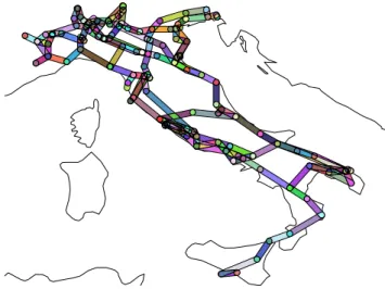
Geometric probability [16] allows us to assign a measure to sets of disks. This measure is simply defined as the Lebesgue integral over the set of disk centers. Using this measure and tools from computational geometry, we can find the probability a randomly located disk that intersects C also intersects some set of links. See Fig. 1 for a simple example and Fig. 2 for an example with respect to the Italian high-voltage electrical transmission network (HVIET).
After this initial failure, due to power flow constraints, a cascading failure may occur. We will use the same power flow and cascading failure model described in [5]. Thus these geometric probability tools along with the cascading failure model allow us to analyze the effects of large scale randomly located disasters on the power network.
We now present our failure model for power flows and cascading failures in power networks. We use the same models as found in [4], [5] and even borrow some notation. The details of the DC power flow and cascading model may be skipped and the reader may proceed to Section III-B without loss of continuity.
1) DC Power Flow Model: We now describe the DC
power flow model which is a linearized version of the more complicated AC power flow model. We use the DC model because it is more tractable and easier to find solutions for power flows.
Let βi represent the amount of power injected at node i.
If βi>0 then node i is a source of power and may represent
a generator where power is injected into the system. If βi<0
then node i is a sink of power and may represent demand at this node. We call these type of nodes power demand nodes. If βi= 0 then power is neither injected or removed at node i
and may represent a power bus. Let N be the set of nodes in the network.
Fig. 2. Every shaded region above represents a set of disk centers whose radius is ≈8
kilometers and only intersects a particular set of power lines should a failure be centered within that region. The network being represented is the Italian high-voltage electrical transmission network (HVIET) [14], [15].
Let (i, j) denote the power line from node i to node j
and let E denote the set of all these lines. Let xij denote the
reactance of (i, j) and let uij denote the capacity of(i, j).
A DC power flow can be described by the amount of power to flow from node i to node j on (i, j), denoted by fij, and
the phase angle at node i, denoted by θi. A DC power flow
must obey the following constraints.
X
j:(i,j)∈E
fij = βi ∀i ∈ N (1)
θi− θj = xijfij ∀(i, j) (2)
Equation (1) constrains the total power out of a node to be equal to the amount of power injected at that node (power conservation). For example, if a node is a generator then the net power flow out must be the amount of power generated at that node. Equation (2) is the analogue to Ohm’s law; the amount of power through a power line is proportional to the difference in phase angles θi and θj.
It should be noted that the power flow has a feasible solu-tion as long as Pi∈Kβi = 0 for every connected component
K in the network (that is, aggregate supply equals aggregate
demand for that component) [5]. Additionally, the values of the power flows are unique [5].
2) Cascading Failure Model: We now describe the
cascad-ing failure model. Again, this model can be found in [4], [5], but is presented here for completeness.
Before any failures occur, we assume the network is connected and that Pi∈Nβi= 0. In other words, we assume
aggregate demand is equal to aggregate supply.
We now describe the cascading failure model in steps. 1) Set ˜fijto be the absolute value of the power flow on(i, j)
2) Consider some subset of power lines to be initially removed from the network.
3) In order to calculate DC power flows for this modified net-work, aggregate supply and demand must match in each component. Hence, we proportionately reduce supply (or demand) at nodes in each component until this condition is met. This may model load shedding or a ramping down of generators.
4) Power flows fij are then calculated for the remaining
network by finding the unique power flows that satisfy equations 1 and 2.
5) Let ˜fij= α|fij| + (1 − α) ˜fij.
˜
fijrepresents some ‘moving average’ of flow through the
power line (i, j) and can be thought of as modeling of
some thermal effects. α is a parameter in this moving average set to a value between 0 and 1. If α is small, then the line will take more time steps to ‘heat up’; if
α = 1 then the line can be thought of as feeling the
effect of the new flow instantaneously. In this work we assume α= 0.5.
6) We then remove all lines for which ˜fij > uij. This may
cause an additional change in the power flows (hence the cascade); we go back to step 3 and the process repeats until no flow is above capacity.
It should be noted that we were not able to attain the capacities of power lines for real power networks. Hence, in order to approximate the capacities on a power network we calculate the initial power flows on each line and then set uij proportional to |fij| before any failures occur. This
proportion is called the Factor of Safety (F oS) and relates to the amount of ‘spare capacity’ on the power lines. In other words uij = |fij| × F oS before any failures occur. For real
power grids, it is believed that a good approximation for F oS is 1.2 [4]. Hence, for the majority of this work, we assume
F oS = 1.2.
B. Performance Metrics and Numerical Results
Our goal is to analyze the effect of a randomly located circular disk failure in conjunction with cascading failures on power networks. Let the yield be the fraction of demand satisfied after the disaster and resulting cascade. By calculating the probabilities of relevant joint link failures using the tools and equations in [11] and considering the resulting cascading effects, one can evaluate the expected value as well as the distribution of the yield to a randomly located disk failure event.
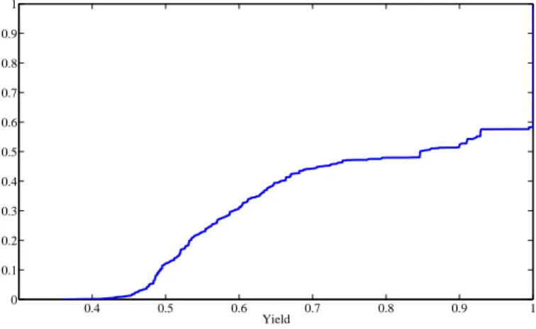
We now discuss some numerical results based on the HVIET network1. Fig. 3 shows the cumulative distribution
function (CDF) of the average yield on the HVIET network with disaster radius of 50 kilometers. Addressing the effect of Factor of Safety, Fig. 4 shows how average yield changes as the factor of safety (F oS) is changed (Factor of Safety relates to the amount of ‘spare capacity’ on power lines). Note when F oS = 1, then there is no spare capacity allocated on
the power lines, so when a failure event occurs the resulting cascading failure brings down most of the network. As F oS increases, the amount of spare capacity on the power lines increase, so the average yield increases as well, as one would 1We would like to thank the authors of [14], [15] for sharing their data.
0.4 0.5 0.6 0.7 0.8 0.9 1 0 0.1 0.2 0.3 0.4 0.5 0.6 0.7 0.8 0.9 1 Yield
CDF of Yield on HVIET network with radius ≈50km, FoS=1.2, and α=0.5, Average Yield = 0.78336
Fig. 3. CDF of the average yield on the HVIET network with disaster radius of approximately 50 kilometers. We assume that the region of interest is given by the convex hull of the network. Note that there is a significant probability the yield is 1; this is mainly caused by disks centered within the region of interest that do not intersect the network.
1 1.1 1.2 1.3 1.4 1.5 1.6 1.7 1.8 1.9 2 0.1 0.2 0.3 0.4 0.5 0.6 0.7 0.8 0.9 1 FoS Average Yield
Average Yield vs. FoS on HVIET network with radius ≈50km and α=0.5
Fig. 4. Average yield vs. FoS on the HVIET network with disaster radius of approximately 50 kilometers. When the F oS = 1, then there is no spare capacity
allocated on the power lines, so when a failure event occurs the resulting cascading failure brings down most of the network. As FoS increases, the average yield increases as well, as one would expect. Note when F oS= 2, then the failure event will have a
much smaller effect on the yield.
expect. For example, when F oS= 2 the failure event will not
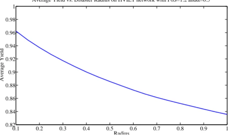
have much effect on the yield. Addressing the effect of the radius of the disaster, Fig. 5 shows as the radius of the initial disaster increases, the average yield in the network decreases. We now compare the effect of independent random link failures to the effect of a randomly located circular failure. We initially calculate the average yield of HVIET to a circular disaster while the size of the region of interest C varies. The size of C is varied to change the probability a unit of fiber is cut. So we can plot average yield versus the probability a unit of fiber is cut. See Fig. 6 for results.
Next, we calculate average yield assuming independent link failures such that links fail with the same probability as in the random disk-cut case. Thus the probability a link fails is still a function of its length, however links fail independently. Since the total number of power lines is not small, calculating average yield by enumerating all possible failures is not feasible (possible failures are exponential in number of links). Instead we use a Monte Carlo approach, using 4000 samples
0.1 0.2 0.3 0.4 0.5 0.6 0.7 0.8 0.9 1 0.82 0.84 0.86 0.88 0.9 0.92 0.94 0.96 0.98 1 Radius Average Yield
Average Yield vs. Disaster Radius on HVIET network with FoS=1.2 and α=0.5
Fig. 5. Average yield vs. radius (in terms of degrees of latitude/longitude) on the HVIET network. As the radius of the initial disaster increases, the average yield in the network decreases. 1 1.5 2 2.5 3 3.5 4 x 10⁻³ 0.88 0.9 0.92 0.94 0.96 0.98
Probability of Unit Link Failure
Average Yield
Average Yield vs. Probability of Unit Link Failure for radius ≈8km, FoS=1.2, and α=0.5
independent link failures geographically correlated failures
Fig. 6. The solid line shows average yield in HVIET versus the probability a unit (latitude/longitude) of power line is cut by a random disk of radius approximately 8km. The dashed line shows average yield in HVIET assuming power lines fail independently such that lines fail with the same probability as in the random disk case.
for each particular probability of unit link failure sample point. See Fig. 6 for results.
Notice that average yield under independent failures is less than in the case of random disk-cuts. This result demonstrates geographic disasters on power networks have key differences from independent smaller scale failures (e.g. power line failure due to brush growth). Perhaps this is because some power supply nodes and power demand nodes are near each other and so a random disk may be more likely to effectively remove both these nodes simultaneously which may reduce the chances of a large cascading failure (since power loads will remain balanced). Also note the contrast to the result in [11] for the NSFNET data network where independent failures on a data network have less impact than in the case of random disk-cuts; this highlights a fundamental difference in the survivability between power and data networks.
C. Possible Extensions
In the context of random geographic failures and power networks, the following problems are potential extensions for future work.
Other metrics: Consider other metrics beyond yield such as the distribution of number of lines destroyed or the distribution of connected components. These distributions will allow us to better understand the impact of a random geographical disaster on the survivability of the power grid.
Computationally efficient algorithms: Development of ef-ficient algorithms to calculate the yield in general networks that scale well with network size. Analyzing the running time of our current algorithms and developing faster methods will allow us to obtain numerical results on larger and more detailed real-world power networks.
Extending the probabilistic failure model: Currently, our model assumes that every power line intersected by a circular disk is removed from the network. However, power lines within a disaster region may not always fail (e.g. shielded power lines near a hurricane may remain operational). So the disaster may have a probabilistic effect on the lines. It would be interesting to capture this doubly random effect; we model a disaster as a randomly located disk that also has a non-deterministic effect on the intersected power lines.
AC Power Flow Model: A more realistic power flow model can be considered. Currently, many papers on power networks assumes a DC power flow model [6] [4]; this type of model is very simple and ignores certain effects that may occur during a cascade. The AC power flow model is a more realistic flow model, though it is harder to solve for the flow equations [12]. We can alter our failure model to incorporate the more realistic AC power flow model and study the impact of the cascading model on yield and other performance metrics.
Robust Design: In addition to the above items, we can study some power network design issues. One goal may be to increase the average yield in the network under a random circular disk disaster. To this end, we may consider how to add additional power lines or increase capacities of certain power lines in order to increase average yield. For example, we may consider what Factor of Safety is required to guarantee the expected yield above a certain threshold.
IV. RELIABILITY OFDEPENDENTNETWORKS
Many systems and networks depend on reliable delivery of power from the electric grid. For example, power is required to operate street lights for transportation networks in cities. Another example are fiber networks; power is needed at backbone routers and amplifiers (on fiber links) or else those components will fail. Since cascading power outages can be widespread, their effect on dependent systems can be devastat-ing. In particular, due to the widespread nature of blackouts, continental fiber networks may become disconnected if the power failure affects a large area that includes the networks physical components. For example, the blackouts of 2003 had a significant effect on the connectivity of the Internet [9].
Motivated by the dependencies of many networks and sys-tems on the power network, we consider the design of robust infrastructures with respect to cascading power failures caused by a randomly located geographic disaster. We first describe a model for the dependence of a network on the power network. We then present our failure model and compare data network reliability with and without power network dependency.
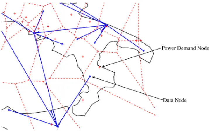
Data Node Power Demand Node
Fig. 7. Part of the backbone of the Italian research network (GARR) [14], [15] is shown above by solid line segments representing links and circles representing nodes. The dashed segments represent the Voronoi cells based on the locations of power demand nodes, shown by crosses above, in the Italian high-voltage electrical transmission network (HVIET) [14], [15]. Our model assumes that data nodes extract power from the closest power demand node; when a demand node fails, data nodes located within its Voronoi cell are assumed to fail as well.
A. Dependence on Power Network
As described above, many networks and systems require power to operate properly; that is, failure to provide power to systems can cause failure in those dependent systems. Although these systems typically have backup power supplies, backup generators are often unreliable. We assume, as in the previous section, that the power network is represented by points and line segments in the plane. Similarly, we assume the dependent network is also modeled by points and line segments. A dependent node is likely to draw its power from a nearby substation. So, we let a dependent node be operational if the closest (in a Euclidean sense) power demand node is still delivering power (that is βi <0 for node i). Thus, based on
the locations of demand nodes in the power network, we can construct a Voronoi diagram; a dependent node in a particular Voronoi cell will depend on the operation of the power demand node corresponding to that cell. See Fig. 7 for an example.
B. Failure Model
We use the same failure model for the power grid presented in the previous section augmented with data-power network dependency. This failure model consists of three stages; the first stage is link failures caused by the random circular disaster and the next stage is the resulting cascading failures in the power network. Then, the effects on the dependent network (based on geographical proximity to supply nodes) are considered once the cascading failures have occurred.
C. Metrics for Dependent Network Robustness
Our goal is to assess the reliability of networks to failures in the power grid. In the context of a random geographic failure on the power grid and the resulting impact on dependent networks, we propose to consider the following metrics:
• Connectivity - In many networks, especially data net-works, we are concerned with connectivity; i.e. does the network remain connected. For example, we would like for all major U.S. cities to be able to communicate with each other, therefore it is reasonable to consider
0 0.1 0.2 0.3 0.4 0.5 0.6 0.7 0.8 0.9 1 0.75 0.8 0.85 0.9 0.95 1 Radius ATTR
ATTR vs. Radius for GARR Network
Power Network Dependency (FoS=1.2 and α=0.5) No Power Network Dependency
Fig. 8. The red dashed curve shows AT T R for the Italian research network (GARR) as a function of the radius (in latitude/longitude coordinates) of a randomly located circular disaster when no power networks are considered (using tools and models from [11]). The blue solid curve shows AT T R for the GARR network when the dependency effects of Italian high-voltage electrical transmission network (HVIET) are considered. For every radius considered a Monte Carlo approach with 4000 samples was used. We note that AT T R is significantly lower when power network dependency is considered; this implies power network effects have a significant impact on the survivability of real-world data networks.
the connectivity of the continental fiber network. Thus, we can consider the probability that the dependent network remains connected after a randomly located disaster on the power grid.
• AT T R - If a connected network cannot be guaranteed
after a failure or full connectivity is not critically important, it may be useful to consider the AT T R metric. This is given by the probability a randomly chosen pair of nodes in the dependent network remain connected after a randomly located disaster on the power grid. In the following, we consider the effect of random disasters on real-world dependent networks using this metric.
D. Numerical Results
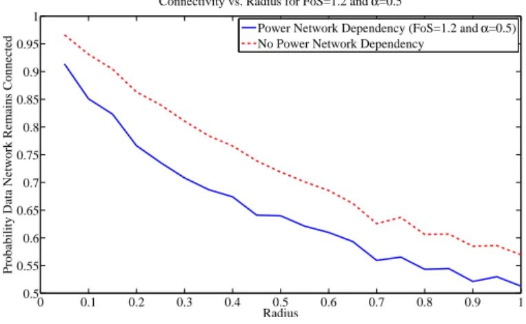
Using the failure model just described, we present some nu-merical results based on the Italian research network (GARR) and the Italian high-voltage electrical transmission network (HVIET) [14], [15]. Consider Fig. 8. Via a Monte Carlo simulation, this figure shows how AT T R is significantly lower when power network dependency is considered; this implies power network effects have a significant impact on the survivability of real-world data networks. Fig. 9 shows a similar result when the connectivity metric is considered although the difference is not as significant. Perhaps this is because removing certain power demand nodes from the network causes the network to be disconnected regardless if a cascading failure occurs.
E. Possible Extensions
In the context of a random geographic disaster on the power grid and its effect on dependent networks, one can consider to study some network design problems. One goal may be to increase the connectivity or AT T R metric in the dependent network. To this end, we may consider how to add additional power lines or increase capacities of certain power lines in
0 0.1 0.2 0.3 0.4 0.5 0.6 0.7 0.8 0.9 1 0.5 0.55 0.6 0.65 0.7 0.75 0.8 0.85 0.9 0.95 1 Radius
Probability Data Network Remains Connected
Connectivity vs. Radius for FoS=1.2 and α=0.5
Power Network Dependency (FoS=1.2 and α=0.5) No Power Network Dependency
Fig. 9. The red dashed curve shows the probability the data network remains connected for the Italian research network (GARR) as a function of the radius (in latitude/longitude coordinates) of a randomly located circular disaster when no power
networks are considered (using tools and models from [11]). The blue solid curve shows
the probability the data network remains connected for the GARR network when the dependency effects of Italian high-voltage electrical transmission network (HVIET) are considered. For every radius considered a Monte Carlo approach with 4000 samples was used.
order to decrease the effect of cascading failures in the power grid thereby reducing the effect on dependent networks. For example, we may consider what Factor of Safety is required to guarantee the AT T R metric remains above a certain threshold in the dependent network. Alternatively, we can consider how to augment the existing dependent network so that it becomes more robust to cascading power failures. An interesting future direction would be to study the joint design of the power grid and dependent network as well as explore the tradeoffs between strengthening the power network and the dependent network.
We now discuss a design problem with respect to data networks. Suppose we wish to strengthen the connection of the data network of two major American cities under the context of random power failures caused by an attack. One problem would be to consider a maximally blackout disjoint path problem: how to find a pair of data paths with common source and destination that has the minimum probability of being affected by a blackout. The solution to this problem gives the most survivable pair of paths with respect to power blackouts.
V. CONCLUSION
Motivated by the effects of natural disasters such as ge-omagnetic storms [13] and cascading failures, in this paper we considered a two-stage failure model for power networks. The first stage removes power lines that intersect a randomly located disk and the second stage calculates the cascading failure that occurs due to the removal of the initial links. We used the tools developed for randomly located circular cuts and a cascading failure model to calculate the effect of this type of failure in power networks. Then motivated by the effects of power loss on data networks [9], we considered the surviv-ability of data networks with respect to power networks. We assumed data nodes rely on the operation of the closest power demand nodes to function. Through numerical results, we were able to show power network effects have a significant impact on the survivability of real-world data networks. Our novel
approach provides a promising new direction for modeling and designing networks to lessen the effects of geographical disasters.
VI. ACKNOWLEDGEMENTS
This work was supported by NSF grants CNS-1017800 and CNS-0830961 and by DTRA grants HDTRA-09-1-005 and HDTRA1-13-1-0021.
We would like to thank the authors of [14], [15] for sharing their data.
REFERENCES
[1] V. Albertson, B. Bozoki, W. Feero, J. Kappenman, E. Larsen, D. Nordell, J. Ponder, F. Prabhakara, K. Thompson, and R. Walling, “Geomagnetic disturbance effects on power systems,” IEEE
transac-tions on power delivery, vol. 8, no. 3, pp. 1206–1216, 1993.
[2] G. Andersson, P. Donalek, R. Farmer, N. Hatziargyriou, I. Kamwa, P. Kundur, N. Martins, J. Paserba, P. Pourbeik, J. Sanchez-Gasca et al., “Causes of the 2003 major grid blackouts in north america and europe, and recommended means to improve system dynamic performance,”
Power Systems, IEEE Transactions on, vol. 20, no. 4, pp. 1922–1928,
2005.
[3] R. Baldick, B. Chowdhury, I. Dobson, Z. Dong, B. Gou, D. Hawkins, Z. Huang, M. Joung, J. Kim, D. Kirschen et al., “Vulnerability assess-ment for cascading failures in electric power systems,” in Power Systems
Conference and Exposition, 2009. PSCE’09. IEEE/PES. IEEE, 2009,
pp. 1–9.
[4] A. Bernstein, D. Bienstock, D. Hay, M. Uzunoglu, and G. Zussman, “Power grid vulnerability to geographically correlated failures - analysis and control implications,” no. EE Technical Report 2011-05-06, 2011. [5] D. Bienstock, “Optimal control of cascading power grid failures,” in
PES General Meeting and submitted to IEEE CDC-ECC11, 2011.
[6] D. Bienstock and S. Mattia, “Using mixed-integer programming to solve power grid blackout problems,” Discrete Optimization, vol. 4, no. 1, pp. 115–141, 2007.
[7] D. Boteler, R. Pirjola, and H. Nevanlinna, “The effects of geomagnetic disturbances on electrical systems at the earth’s surface,” Advances in
Space Research, vol. 22, no. 1, pp. 17–27, 1998.
[8] S. Buldyrev, R. Parshani, G. Paul, H. Stanley, and S. Havlin, “Catas-trophic cascade of failures in interdependent networks,” Nature, vol. 464, no. 7291, pp. 1025–1028, 2010.
[9] J. Cowie, A. Ogielski, B. Premore, E. Smith, and T. Underwood, “Im-pact of the 2003 blackouts on internet communications,” Preliminary
Report, Renesys Corporation (updated March 1, 2004), 2003.
[10] J. S. Foster Jr. et al., “Report of the commission to assess the threat to the United States from electromagnetic pulse (EMP) attack, Vol. I: Executive report,” Apr. 2004.
[11] S. Neumayer and E. Modiano, “Network reliability under random circular cuts,” in Proc. IEEE GLOBECOM’11, Dec. 2011.
[12] T. Overbye, X. Cheng, and Y. Sun, “A comparison of the ac and dc power flow models for lmp calculations,” in System Sciences, 2004.
Proceedings of the 37th Annual Hawaii International Conference on.
IEEE, 2004, pp. 9–pp.
[13] R. Pirjola, “Geomagnetically induced currents during magnetic storms,”
Plasma Science, IEEE Transactions on, vol. 28, no. 6, pp. 1867–1873,
2000.
[14] V. Rosato, L. Issacharoff, F. Tiriticco, S. Meloni, S. Porcellinis, and R. Setola, “Modelling interdependent infrastructures using interacting dynamical models,” International Journal of Critical Infrastructures, vol. 4, no. 1, pp. 63–79, 2008.
[15] V. Rosato and S. C.-K. Chau, personal communication, 2011. [16] L. Santalo, Integral Geometry and Geometric Probability. Cambridge