The baroclinic instability of simple and highly structured one-dimensional basic states

©

THE BAROCLINIC INSTABILITY OF SIMPLE AND HIGHLY STRUCTURED

ONE-DIMENSIONAL BASIC STATES

by

JAMES WILLIAM ANTHONY FULLMER

B.S., Drexel University (1972)

SUBMITTED IN PARTIAL FULFILLMENT OF THE REQUIREMENTS OF THE

DEGREE OF DOCTOR OF PHILOSOPHY

at the

MASSACHUSETTS INSTITUTE OF TECHNOLOGY MAY 1979

) James William Anthony Fullmer

Signature of Author ... Department of Meteorology, May 1, 1979

Certified by ... Thesis Supervisor

Accepted by ... Chairman, Departmental Committee

on Graduate Students

MIT

_LIBRARIES

EBRARIES

i i ~ u III THIS THESIS IS DEDICATED LOVINGLY TO MY PARENTS Mrs. Antonine H. Fullmer Mr. James M. Fullmer l IYIIIYII ii Y

O<v

actre

0)0

1%

M(CLt

)

₁

_po

_D

_st(

Ko C~

I

'SO(

tro

oo( OV

A R r

To

PHAANE

"A

e

C/o

vdr"

423

.c.

\We

sh oll

iqot

cease

from

ex

pfora

Ar\de

+e

Will

Le

en

d

of

l0.11

to

our

where

explo-

tng

we

stalred

f 6e

_place

for

hke

fs

_time.

Four QuarieIs

)gEpoU

t%

Ierepoc

To

vov#ko

Sejo a .

ton

Anda

rill~l IIYYYYIY IYYIIYIYIYYII

r,

%y14

c

er

o0'

s

3) I1

Ar

S

~E~-C~V

T.S. ELIOT

_{143 A..}

6911

by

JAMES WILLIAM ANTHONY FULLMER

Submitted to the Department of Meteorology on 1 May 1979 in Partial Fulfillment of the Requirements for

the Degree of Doctor of Philosophy

ABSTRACT

The baroclinic instability of simple and highly structured one-dimensional basic states is studied using a frictionless, adiabatic, quasi-geostrophic model on a s-plane. Square-root-pressure coordinates are used at 48 levels in the vertical and calculations are made for the upper boun-dary conditions 4' = 0 and w' = 0. Many properties of the unstable waves are considered: instability source, wavelength, growthrate, phase velocity,

steering levels, and the vertical structure of their amplitude, phase, meridional entropy transport, and potential to kinetic energy conversion.

First, simple basic states are assumed. Their shear and static stability each have a single value from 1000 to 250 mb, and another, independent value from 250 to 0 mb. These simple basic states are determined by 3 parameters: a shear ratio, a static stability ratio, and a generalized

8

parameter. A wide expanse of parameter space is considered. The highly structured basic

states have zonal velocities and static stabilities obtained from one month averaged data for latitudes 250N to 650N and for months (January, April, July, and October), which represent seasonal extremes and transitions.

The longwave modes discovered by Green (1960) are shown to have several interesting properties. To exist, they require a non-zero value of qy and are destabilized by the presence of a Stratosphere or rigid lid. Doubling times are moderately short (about 1 week) and their meridional cir-culation in the lower stratosphere agrees with observations. Pressure

ampli-tudes, kinetic energy destruction, and meridional entropy transport are par-ticularly strong in the lower stratosphere (relative to other levels).

Their kinetic energy is generated in the troposphere. Their entropy trans-ports are countergradient in the lower stratosphere when a reversed shear

exists in that region.

Quasi-geostrophic potential vorticity meridional gradient profiles (qy) for the one month averaged data possess a considerable number of zeros. These zeros and their associated negative qy regions have a substantial

ef-fect on the unstable mode spectrum._ Some modes' growthrates are drastically reduced when a particular negative qy region is removed. New modes (dis-tinct from those discovered by Eady, Charney, and Green) exist only when certain negative qy regions are present. Some of the new modes are

poten-tially important for the general circulation of specific regions of the atmosphere. In particular, longwave modes, in addition to those discovered by Green, could be important for the stratospheric circulation, and some are examples of in situ stratospheric baroclinic instability.

5

The unstable mode spectrum is also shown to be sensitive to small changes in the unperturbed state. It is shown that only those changes which drastically alter the negative regions and associated zeros of the qy profile result in a substantial change in the unstable mode spectrum.

TABLE OF CONTENTS

ABSTRACT ... 4 TABLE OF CONTENTS ... 6

I. INTRODUCTION ... 8

1. Background and problems to be addressed 8

2. Outline of the thesis 13

II. THE MODEL ... .... ... 16

1. The model eigenvalue equation 16

2. Boundary conditions ₁₈

3. Fluxes and energetics 20

4. Numerical Accuracy ₂₂

Figures 26

III. TWO-LAYER MULTI-LEVEL MODEL RESULTS ... ... ... 32

1. Introduction and overview 32

2. Necessary conditions for baroclinic instablity 33

3. Nominal parameter values 35

4. Results for special and nominal parameter values 36 5. _{Results for the variation of one parameter with}

others fixed at nominal values 40

6. Results for constant ^(T planes in parameter space 45

7. Calculations for w'=0 at p=0 49

Figures ₅₅

IV. RESULTS FOR THE HIGHLY STRUCrTURED BASIC STATES...114

1. Introduction 114

2. Criteria for choosing input data for the model 115

3. The data sets ₁₁₆

4. Calculation of q1 117

5. Processing the dAta for input to the model 120 6. Model results-classification of modes 122

7. The Eady modes ₁₂₅

8. The Green modes 127

9. The E_s and S_m modes 130

10. The S modes ₁₃₁

11. The L modes 133

12. The necessary conditions for instability and the

existance of unstable modes 135

13. Importance of the unstable modes to the general

14. Calculations for w'=O at p=O Figures Tables 143 145 194

V. SUMMARY OF IMPORTANT RESULTS ... 217

APPENDIX ... ... ... 220

ACKNOWLEDGEMENTS ... ... ... . .... 229

REFERENCES ... 231

CHAPTER I INTRODUCTION

1.1 Background and Problems to be Addressed

One of the oldest and most interesting problems of dynamic meteor-ology is the stability of a horizontally uniform steady flow. The flow is

said to be baroclinically unstable when there exist perturbations which grow exponentially with time, and which derive their energy from the available potential energy of the mean zonal flow. Investigation of the baroclinic in-stability problem began with the works of Charney (1947) and Eady (1949). Eady's model assumed a linear velocity profile, no variation of the corio-lis parameter (P3= 0), and rigid lids at the top and bottom. Unstable modes were found above a certain wavelength. Charney's model atmosphere had a rigid bottom but an unbounded top. A linear velocity profile was assumed

(with the velocity constant above a certain height) and variation of the coriolis parameter was permitted. Charney found instability only for waves shorter than a certain wavelength which depended on the value of P (or on the value of the wind shear).

Burger (1962) established for a continuous model with constant p 3 0 that all wavelengths have an exponentially unstable mode associated with them except for certain isolated wavelengths. Modes on the longwave side of these isolated wavelengths always grew more slowly than those on the shortwave side.

Green (1960) in a numerical model had also found that all resolved wavelengths were unstable (with the exception of isolated wavelengths) when

P

#

0. Green also extended Eady's and Charney's results to include a

--infinite "stratosphere" of increased constant static stability. The shears however, was kept uniform throughout his atmosphere. The effect of the "stratosphere" was to make longer waves more unstable. His growth rate spectrum is similar to that for SR = 1 in Figure 3.4, given below. The shorter modes to the right of the cusp point in Figure 3.4 will be referred to as Charney or Eady modes. Those on the other, longwave side will be called Green modes.

Green showed that the fastest growing Eady mode did not have much vertical structure. However, Geisler and Garcia's (1977) numerical calcula-tions found the Green modes to have streamfunction amplitudes in the stratosphere

an order of magnitude larger than those in the troposphere. Geisler and Garcia assumed a reference state temperature characteristic of a mid- lati-tude winter, and both a linear and a mid-latilati-tude winter mean zonal velo-city profile. Both Green and Geisler and Garcia found growth rates of the Green modes to be much less than those of the Eady modes. However, there is no certainty that modes of largest growth rate must dominate. In fact, Gall (1976) and Staley and Gall (1977) have shown that the longer unstable waves can have a longer time to grow than the shorter waves because they extend higher into the atmosphere to regions where their growth is not halt-ed as quickly by interactions with the mean flow (see also the discussion in Section IV-13). The Green modes, therefore, could be of great importance to the upper atmospheric circulation. Many of their properties remain un-investigated; in particular, their kinetic energy release and entropy trans-port. Also uninvestigated is the dependence of the vertical structure of these waves on 6, the shear of the mean zonal flow, and the static stability. The study of these properties of the Green modes is one major concern in this thesis.

One- of the properties of the baroclinic modes which is essential to the atmospheric general circulation is their transport of heat. The trans-port is generally poleward and upwards, down the horizontal gradient of the mean temperature (Oort and Rasmusson, 1971), and accounts for a substantial part of the total heat flux at mid and high latitudes (Oort, 1971; Palmen and Newton, 1969, pp. 62-63). The eddy heat fluxes prevent the occurrence of very large meridional temperature gradients and associated intense west-erlies. The theoretical study of Stone (1972) shows that the baroclinic eddies are essential to the determination of the atmospheric temperature structure. The studies of Phillips (1954) and Kuo (1956) show that the

eddies help drive the mean meridional circulation. Models of the atmosphere, consequently, must include the effects of these baroclinic eddies.

The lower stratosphere (from the tropopause to 30 mb) presents a cur-ious exception to the general description of atmospheric heat flux given above. Murgatroyd (1969) points out that the latitudinal heating gradient opposes the latitudinal temperature gradient in winter and summer and this requires a net countergradient meridional heat flux. The contribution of the mean meridional circulation to the horizontal flux has been calculated from observations of Oort and Rasmusson (1971) at 100 mb. At this level, the mean flux tends to be weaker (by a factor of 4 or more) than either the transient or stationary eddy flux and is generally equatorward. However, the observation of Oort and Rasmusson (1971) and Newell et al. (1974) show the eddy heat fluxes to be poleward up to 10 mb and countergradient between the tropopause and 30 mb. The transient eddy fluxes are about 1/2 to 2/3 as strong as those of the stationary eddies. Newell (1964a) has described

the lower stratosphere as a refrigerator which maintains the temperature minimum at the equator through countergradient eddy heat fluxes.

The origin of the observed lower stratosphere net countergradient heat flux has not been determined. The lone observations of Oort and Rasmusson at 100 mb are not strong enough to discount the mean meridional circulation from playing an important role in determining the net heat flux. The non-interaction theory begun by Charney and Drazin (1961) and extended by Holton (1974) , Boyd (1976) and Andrews and McIntyre (1976) tequires that, in the absence of diabatic effects and dissipation, the heat (and momentum) fluxes of stationary eddies (even if these eddies have harmonic time variations) are

exactly balanced by transports of an induced mean meridional circulation. Thus, only transient eddy motion or a circulation in which diabatic or dissipative effects are important remain as candidates for producing the net countergradient heat flux in the lower stratosphere. Diabatic heatinq rates are small in the lower stratosphere (< .50

K/day; Newell et al. (1969), Murgatroyd (1969), Houghton (1978)) but still may be important to the heat budget (Vincent, 1968). Viscous dissipation is likely to be small compared to radiative damping (Holton, 1975). Although a circulation with diabati-city and possibly dissipation is a possible mechanism for generating the net countergradient heat flux, this mechanism is outside the scope of the current study.

The transient eddy component o the net countergradient heat flux is unlikely to come from in situ stratospheric baroclinic instability (Holton

(1975), Simmons (1972)). Most of the transient eddy activity in the lower stratosphere, Holton claims, is probably due to the remnants of baroclini-cally unstable modes which originate in the troposphere. Green (1960) and

Peng (1965) have shown by numerical studies that the heat fluxes of the dominant Eady mode are very weak in the stratosphere. Green's (1960) fluxes for the domi-nant Eady mode were down gradient as he did not consider the reversed

strato-spheric temperature gradient. The strength of the Green mode amplitude in the stratosphere and the results of Gall (1976) mentioned above, indicate that these

modes may possess strong stratospheric heat fluxes. The possibility that these fluxes may be significant and countergradient will be investigated, and impli-cations for the parameterization of stratospheric eddy heat fluxes will be discussed.

Necessary conditions for baroclinic instability were derived by Charney and Stern (1962) . They found that, in the absence of boundary temperature gra-dients, the quasi-geostrophic potential vorticity gradient (q y) profile must possess a zero for baroclinic instability to occur (for a more detailed

discus-sion of this result, see section 111-2). The calculations of Leovy in Charney and Stern (1962) show zeros in q above 100 mb for data of 14 October, 1957. Leovy and Webster (1976) also suggest that qy may also have zeros on the tropical side of the stratospheric jet. Furthermore, Charney and Stern (1962) showed that

such zeros are necessary conditions for an internal instability; they, as well

as Green (1972) , McIntyre (1972) , Simmons (1972, 1974) and Dickinson (1973) have shown that a zero in qy is a sufficient condition for instability in a number of special cases. Therefore, detailed profiles of u and T, closer to those found in the atmosphere than the simple linear profiles studied by previous authors, may possess zeros in which have associated unstable modes. Detailed profiles

of u and T are also of interest because small variations in their detail have been shown to alter significantly the growth rate spectrum of the Eady modes

JGall and Blakeslee, 1977; Staley and Gall, 1977). In this thesis, the,

effect of the structure of the u and T profiles on the baroclinic insta-bility problem will be considered along with the sensitivity of the results to small variations in these profiles.

1.2 Outline of the thesis

The problems raised in the discussion above will be addressed through a comprehensive study of the baroclinic instability of both simple and highly structured one-dimensional basic states. Many properties of the unstable waves are considered: instability source, wavelength, growth rate, phase velocity, steering levels, and the vertical structure of their pressure amplitude, phase, meridional entropy transport and kinetic energy genera-tion. The model used is the quasi-geostrophic s-plane model of Green (1960) written in square-root-pressure coordinates. This choice of vertical coor-dinate gives an equal number of levels in the upper layer (stratosphere) and lower layer (troposphere). The upper layer is thereby given sufficient resolution without having an unnecessary number of levels in regions of very little mass. In Chapter II the mathematics of the model are devel-oped and the numerical accuracy of the integration scheme is checked.

This study first extends Green's results by a "two-layer multi-level model" (Chapter III). Within each layer, the shear, u , and static

stabil-1 d In 8

ity, P P dp , are constant but can have independent values. A 3-parameter family results. In addition to Green's generalized

8-parameter,

- 8o Poo2 up (upper layer)

Y , there is a shear ratio SRer layer) and static

sta-T

f2u₀ u (lower layer)

r (upper layer)

bility ratio a (lower layer) Green's assumption of the same shear in both layers has been relaxed. A wide expanse of the three-dimensional

* Klein (1974) addressed the same baroclinic stability problem, but confined himself to profiles of zonal wind and temperature which are characteristic of a mid-latitude winter. In addition, he was restricted by his method of analysis to only the most unstable mode at each wavelength.

parameter space is explored. The dependence of the Eady and Green mode's properties on the parameter values is studied in detail. In particular, it is shown that the Green modes do have strong countergradient heat fluxes in the lower stratosphere although nearly all of their kinetic energy is

drawn from the troposphere.

Chapter IV presents a further extension of Green's model to more realistic u and T profiles for the basic state. The profiles are obtained from monthly averaged data at different latitudes and are one-dimensional. One cannot rigorously justify using monthly averaged data for the unperturbed state, since the u and T profiles from monthly averaged data do contain the effects of atmospheric eddies, and the unperturbed flow does not vary on a much slower time scale than the eddies. Nevertheless, the use of monthly averaged data for the unperturbed state can be viewed as a reasonable way

of relaxing the simplified representation of u and T in previous baroclinic

instability studies. It is a reasonable "next step" which allows one to, see how the unstable modes are affected by detail in the structure of the basic state.

The one-dimensionality of the basic state is justified partly by the work of Moura and Stone (1976). They found that if the unperturbed state is locally unstable, it is globally unstable. Local conditions (e.g. at a single latitude) are important in determining instability even if meridional variations are included and if the unstable modes have large meridional

scales. The one-dimensional basic state is also justified by the secondary role that the meridional variations are found to have in determining the

will show that vertical variations alone represent well the features of the qy profile which are important in determining stability properties.

As in Chapter III, the Green and Eady modes are studied in detail, and the Green mode is again shown to possess strong countergradient heat fluxes in the lower stratosphere. In addition to the Green and Eady modes, other long and short wave modes are shown to exist for the more detailed u and T profiles. This reveals an advantage of the eigenvalue approach over the numerical time integration approach. The latter gives only the most unstable eigenvalue at each wavelength; the former gives all the unstable modes. Many of the new long and short wave modes are shown to exist only when certain negative qy regions exist. The existence of negative qy regions is shown to be very sensitive to small variations in the basic state. In-deed, small variations in the basic state are shown to affect the unstable mode spectra significantly only when they result in changes in the depth and location of negative qy regions.

Most of the model calculations were done with the upper boundary con-dition

9'

= 0 at p = 0 (?' is the perturbation stream function). However, to allow for a possible source of instability at p = 0, results assuming W' = 0 at p = O0 are presented and explained whenever these differ signi-ficantly from those assuming

Y'

= 0 at p = 0. Chapter II discusses the choice of the upper boundary condition in more detail.

CHAPTER II

THE MODEL

2.1 The Model Eigenvalue Equation

The quasi-geostrophic model on a a-plane is well-suited for the purposes of this study. It is simple enough to allow a detailed parameter study of large-scale motions and it still provides a good approximation to the properties of such motion. The equations for such a model, written in

7 = (p) coordinates, n being an arbitrary function of pressure, are:

-- ( f + ) = f w' ₍₁₎ Dt o (1 D cr Tr' - (2) Dt - f 0

where x, y, t are the eastward, northward, and time coordinates,

4

is the horizontal streamfunction, f = fo + By is the Coriolis parameter, a =

1 d in 6s is the reference state static stability, _dp is the vertical

p dp dt

dvelocity, i 2 D

velocity, 7' - = + is the vorticity, and

dp , x2 y2 Dt t

d i d

y dx x dy

One next non-dimentionalizes with scales p - poo x,y - L, , ~ Lu0

L PooUo

t - , w . Then, following Phillips (1954), one defines:

uo L

S= + qp'

ik (x-ct) ' = Y(T) cos y e

x yy = 0

Stime variation of the mean flw, is hen of o

17

above substitutions, the differential equations become:

(T - (u-c) p2) = TP TP2~

7

T

ik

fL2u dTr (3)

[

TPoo 1

(u-c) T - uf =

mi-

(4)

T 7T i fL2UO

where all quantities except those in brackets [ ] are non-dimensional and

B aTPoo 2 2 (k2+p2) TPoo2

Y - is the generalized P parameter, and P - 2 is

T - f2Uo f

the non-dimensional wavenumber. Using Phillips' 1954 grid, one writes the vorticity equation at odd levels and the thermodynamic equation at even levels. Combining these finite difference equations as Phillips did results

in: i 0 = T (u -c2)P2) _ - H (u -c) - (u -c T T-n -- n n n-2 n n n+2 n

(5)

+ Z T (u -c)T + + + (u -c) n n n n-2 n n n n+2

where n is odd and runs from 1 to N-1 = 97 (N is defined as the value of n at the ground level and equals twice the number of levels at which ~ is written),

means the value of ( ) at level n, n

Sr I 1i 7 TI +

+ n n+l

p-

n n-l and

En

T/nl

n ( )2 n (A) 2 nl

With appropriate boundary conditions (discussed below), eigenvalues of this system of equations are found by the OR algorithm. The algorithm

is one of the most efficient methods known for solving the complete eigen-value problem for symmetric or non-symmetric matrices (Dahlquistand Bjbrck,

1969). It is most efficient if the matrix value whose eigenvalues are desired is in Hessenberg form. The eigenvalue matrix is balanced, and put into Hessenberg form and solved for its eigenvalues by EISPACK subroutines

*In the equations and symbols below aT is the nominal tropospheric value of c given in Section 3.3.

_____ ____ ... _IIn ImrI iIl_____

provided by the MIT Information Processing Service (IPS). The IPS publica-tion AP-42 describes these subroutines.

Eigenfunctions are obtained by assuming Real[j3 = Real ₂l = 1 if the boundary condition is t' = 0 at the top, or by assuming RealY ₃ =

Im3 = 1 if the condition is

P'

= 0 at the top. The eigenvalue equation is then used to integrate downwards. The homogeneity of the eigenvalue equation justifies the arbitrary choice forY1 _orY3.

2.2 Boundary Conditions

At the bottom _{0. This is justified because in the first} approxi-mation for quasi-geostrophic motions ) 2 -gpw. In the atmosphere for motions of synoptic or larger scale, the other terms in the & - w equation are small-er by an ordsmall-er of magnitude or more. The &.= 0 lower boundary condition

also filters out horizontally propagating acoustic waves. The lower boun-dary condition is applied at level N. It results in an equation relating

- tofN-3 This relation between ₁ andN ₃ is obtained by writing

N-1 N-3 N-l N-3

the eigenvalue equation (Eq. 5) at level N with

TT+

=0.

N-l

At p = 0, the top of the model atmosphere, both the author and Holton (1975) have found that only the W = 0 boundary condition has been used in the literature for quasi-geostrophic models. While being exact in theory, this condition can act as a rigid lid. It can introduce spurious

free oscillations which may be unstable, and cause reflections of vertically propagating modes (Lindzen,A1968; Cardelino, 1978).

Geisler and Garcia (1977) assumed 4)'= 0 at a level "(typically 100 km) where solutions of interest have already decayed to a negligible value",

their model is in geometric coordinates. Indeed, asymptotic solutions of the quasi-geostrophic equations for U profiles linear with height show that

I

' grows or decays exponentially. Assuming i' =0 ina geometric coordi-nate model retains only the realistic decaying solution. Charney inMorel et al. (1973) requires that the upward energy flux ps 4'w' is zero at z = C. This is satisfied if the decaying solution is selected because lim

ps*$ = lim p k'w'. The assumption behind the upper boundary condition

z s

lim I

j

= lim p P'w' = 0 is that one's solution should decay away from

Z-)c Zo

energy sources which are at finite heights.

For the model used here, problems with up constant have uz ^u -- 0 as z ->, so that the available potential energy goes to zero as z-.o. For this case, which has no energy source near the top, Charney and Pedlosky (1963) have shown that the energy flux of the disturbance will decay at least ex-ponentially with height. The disturbance will then decay to zero amplitude at the top. Thus, T' = 0 is a realistic boundary condition.

Consideration of energy sources above the stratosphere is not with-in the scope of the current study. Calculations, therefore, are presented primarily with Y' = 0 as the upper boundary condition. However, comparisons will be made with calculations which have c' = 0 as the upper boundary con-dition. Important differences in the calculations resulting from the differ-ent boundary conditions will be pointed out and their physics will be discussed.

In particular, it will be seen that the long wave Green mode experiences a behavior analogous to reflection when t' = 0 is used.

Implementation of upper boundary conditions in the reduction of the num-berofmodel levels from 49 to 48 (Figure 2.1 shows the height and pres-sure of model levels). The condition w0 = 0 is replaced by l' = 0 and

the remaining 48 equations at levels 3 to 97 are solved for their eigen-values.

2.3 Fluxes and Energetics

To obtain the horizontal entropy fluxes, one first uses the

hydro-a 1 Poo K

static and Poisson relations: (6);

6

= (°) T (7); and the

ap fo p P

ideal gas law P = pRT (8); to relate 8 to the streamfunction:

fo PooK a _

R P p (9)

The meridional velocity is simply v' =

Ox'

and the vertical velocity is related to ) through the thermodynamic equation. With the additional as-sumption that =even = (m+ + m- ), one multiplies the expressions for

m-even 2 m+l m-l

v and

0,

w and 0, and 0 and 4. Then averaging zonally and simplifying results in: ' 1-K 1 * (v'8') = P kme Real i - IF aT 2 -K 1 A K-l -1 _tan ('8') (--) P kmE ((L)2 -

8

tan y + -u * *

* Real

(i

-'

1

- 2c. Real {(i + T-1 i ++1+ N 1 + c. I P + i 1 -1 -1 ' £+i £+i - ' Lc * * ] k

,

9 4kn - £+ T t+l +l 1 (u + u1 - 2cr ) Real {i -i + +l U1 r E-1 £+1

where m = cos py, = eklit , C and c. are the real and imaginary parts

r 1

of the phase speed and ) is even. Given eigenvalues and eigenfunctions, the above non-dimensional correlations are then computed. The last cor-relation is often called the "pressure work term" for reasons given below.

The quasi-geostrophic energy equations have been derived by Charney (in Morel, 1973) for geometric corrdinates. Their counterparts for pres-sure coordinates are:

dX Poo K 1 d - u'' u dy dp - 'O' ( ) dy dp dt y Ro PO 0 p

''dy

= CK + CE + BE dE

F

U v' u dy dp ( I v - 2K I dt u y d y (o) dy dp P R- f

Jdy

= CK + CA + BE

o

fp

Poo P dy dp - v'' _ y Poo ) dy dp = -CE +CA

where,

=

L /L , (L = is the radius of deformation)

6' r r fZ.

1

= _{i-1 ----} C + C +B ₂

*Note: Once r(p)is known, writing the energy equations in Tr coordinates requires only a very simple transformation.

31,

E

, andA are the Eddy Kinetic Energy, Total Eddy Energy, and Eddy Avail-able Potential Energy, respectively (Lorenz, 1967). The power integral CK, which represents transfer of kinetic energy between zonal mean and eddy flow,

is not present for this one-dimensional model since U = 0. The power inte-gral CA, which represents the transfer of available potential energy between

zonal mean and eddy flows is studied by presenting profiles of the hori-zontal heat flux. The horihori-zontal heat flux has the more direct effect on temperatures. Profiles of the full power integral CE are presented because CE describes the source regions for Eddy Kinetic Energy. The last term, BE, describes the transfer of eddy kinetic energy into or out of a given pressure layer P1 to P2. Since p is always -90° out of phase with v, the

M't'

correlation reveals the relation of poleward to downward velocities

throughout the atmosphere. It will be used to relate model eddy motions to observations.

2.4 Numerical Accuracy

The numerical method described above is a second order scheme, and numerical experiments didshow the error in growth rates varying inversely with the square of the number of levels when7 = P is the coordinate. For nominal values of the stratosphere/troposphere shear ratio, SR = -1.5, and static stability ratio a = 50 (see Chapter III for the calculation 6f these

p

values), Figure 2.2 illustrates the Eady mode's growth rate accuracy as a function

of YT (YT = 2 is nominal). Note that many more levels are needed to obtain accurate growth rates for higher 'T because the most unstable wavelength becomes shorter, and the associated vertical structure becomes finer.

The model resolution of 48 levels is of good accuracy at least to wavenumber P = 6 or wavelength = 1.8 x 103 km. In low latitudes yT can be large and

T

one would need 15 or more levels to even detect instability if YT = 10.

T The results in Figure 2.2 are identical for both upper boundary con-ditions. The Green mode, however, which has the longer wavelength of 8.3 x 103 km (P = 1.3)' for nominal parameter values, is resolved much better when Y'P = 0 is the upper boundary condition. In this case, the doubling time is determined to within 2% of its 48 level value (6.1 days) when only 13 levels are used. However, when w' is the upper boun-dary condition, 37 levels are required for the doubling time to be within

2% of its 49 level value (14.7 days) (the marked differences between these estimates of the Green mode doubling time is discussed with the Chapter III

&)I =

0

calculations). The above and additional calculations showed that when doubling times of long-wave modes were calculated, calculations using

(P'.O

= 0 converged more rapidly than those using the more common Oj('p= = O upper boundary condition.

The ability of the model to converge over the entire range of the vertical coordinate is illustrated in Figure 2.3, which shows results valid

for both upper boundary conditions. For the meridional entropy flux of the Eady mode, good convergence is obtained for the model resolution of 48 levels (49 levels, for the w' = 0 boundary condition).

(p=0)

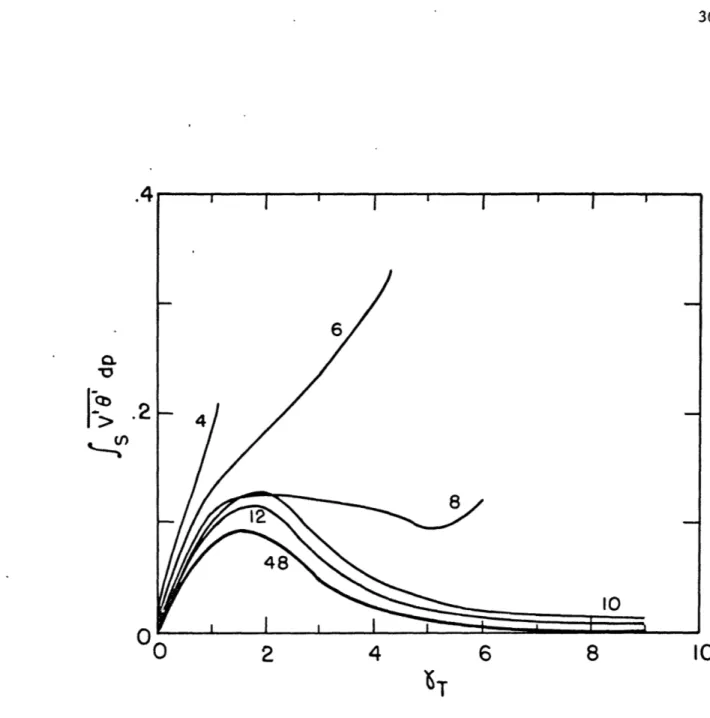
For entropy fluxes of the Eady mode at higher YT values and shorter wave lengths, Figures 2.4 and 2.5 show model convergence (their results are identical for both upper boundary conditions). The quantities v'8' and

T

v'e' are the mass weighted zonally averaged meridional entropy fluxes for s

the troposphere and stratosphere, respectively. Each profile of v'9' has been normalized, i.e. the maximum value for all levels in the profiles has been set equal to 1. Good convergence on values of v'e'T and v'e's exists

for modes with zonal wavelengths as small as 1.8 x 103 km.

Three additional checks were made on model accuracy. The first is a check for satisfaction (numerically) of the lower boundary condition. Both upper and lower boundary conditions were, of course, used to determine the eigenvalues. Determination of the eigenfunctions, however, started with the upper boundary equationY 1 = 0 and assumed an amplitude and phase

forY3 (see the earlier discussion in this chapter for a justification of

this assumption). Then the model eigenvalue equation (Eq. 5) is used to determine values of Y at lower levels. The value of Yat the lowest level,

YN-1' is obtained from the eigenvalue equation written at level N-3, which

relatesL to -3 and y . The remaining Yequation, written at level

N-l N-3 N-5

N-1 contains the lower boundary condition. It must be satisfied by the

N- and N-3 values, which were determined by the eigenvalue equation

N-l N-3

written at higher levels. Satisfaction of this lower boundary equation was checked for all model results.

Asecond check is satisfaction of Howard's Semicircle Theorem Test (see Pedlosky (1964) for application of this theorem to quasi-geostrophic models). All values of the eigenvalues were found to be within the theo-retical limits of the test.

A final check on the model's validity is its ability to reproduce

-1

previous results. A plot of growth rate contours vs

rT-1

and wavelength

2

7r

2for Green's linear u profile reproduces his Figure 3 exactly (see Figure P

2.6 and Green (1960), Figure 3). (w' or w' = 0) at the top.

-- -- 111 111 1 IIIYYIYIYIIIIYIYIYII 1 Yi 100 0-- 0 26 80- -200 60 - 400 E E mb w cE w _w 0. 40- -600 20- -800 km O0 I I I I I I I I I 1000 0 20 40 60 80 98 LEVEL NUMBER

Figure 2.1. Height and pressure of model levels.

1i11hi I IIAtIIId U iIl hIi *I

----27 04 ₄₈ o ₄₄₂ 36 030 24 C: .0 In oC 02 4 6 10 8

Figure 2.2. Growthrate vs. T of the fastest growing Eady mode for

models with indicated numbers of levels for which 4 is written; SR = -1.5, op= 50.

E 484 2 6 4 CL o 600-800 1000I I I .01 1 v 1.0

Figure 2.3. Vertical structure of the meridional heat flux of the fastest growing Eady mode for YT = 2, SR = -1.5, = 50.

29 1.0 i I I

.8

6

.6

8 .10 14

.2-

0

48 0 2 4 6 8 10 6_T

Figure 2.4. As in Figure 2.2, except for the tropospherically integrated meridional heat flux.

~-~I--- - 111 -.lliil 30

4

IIII

6

4

4

10

0

2

4

6

8

10

t

_T

Figure 2.5. As in Figure 2.2, except for the stratospherically integrated meridional heat flux.

2.0

1.5

1.0

0

2

4

6

WAVELENGTH (nondimensional)

PcI

Figure 2.6. Non-dimensional growthrate 1 divided by Y

of Y and wavelength p = 1, SR = 1, u(p=0) = 1, and W' Neutral modes are shown by the heavy zero curve.

Tha o

Neutral

as a function

-M- Y,

32

CHAPTER III

TWO-LAYER MULTI-LEVEL MODEL RESULTS

3.1 Introduction and Overview

This chapter treats the atmosphere as a 2-layer system having a troposphere and stratosphere. Each layer has an independent shear and static stability, and these unperturbed flow parameters are constant within each layer. This approach simplifies the parametric study of how the unperturbed state affects the perturbations. Within each layer are 24 levels so that the vertical structure of the perturbations can be studied in fine detail.

Three parameters completely determine the unperturbed state: Y', the generalized n-parameter, defined in chapter II; SR, the shear ratio

du) du

du stratosphere/

(dptropospher) ; and _{, the static stability ratio} dp stratosphere dp troposphere

/- . The velocity field, u = n ranges from 0 to

stratosphere troposphere n

u_o

p 1 1

1 between ground and tropopause ( - ) and from 1 to 1 + SR between

Poo 4 3 tropopause and p = 0: 4 1 1 - SR p + 3 SR stratosphere U = 4 4 (l-) troposphere

The static stability parameter, = 1 for m > 49 and = 1- , for m <49

m _{mo 'o}

(note: m

$

49,as m is even). When values for YT, SR, and 69 are chosen, the model eigenvalue equation is ready to be solved to any specified non-dimensional wavenumber P.

Solutions will first be obtained for combinations of special and nominal values of the parameters. "Nominal" values are defined as those

11I~~. u~~l

---appropriate for mid-latitude winter conditions: YT = 2, SR = -1.5, and

0-=

50 (these values are calculated below). Special values used are

YT=0 (no -effect),SR = 1 (uniform shear throughout the atmosphere), SR = 0

(no shear above P/ = 1/4), and = 1 (no stratosphere, uniform static stability throughout the atmosphere). Every combination of these parameter values will be studied. This will enable one to see the effects of: uni-form shear, zero shear above p/P_{o o} = 1/4, and nominal shear above P/Poo = 1/4, both with and without a stratosphere, and with and without the ,-effect.

The second part of this parameter study will use the nominal para-meter values to define an origin in parapara-meter space. The study will include parameter values on axes through the origin along each of which only one parameter varies. Both the first and second parts of the parameter study will treat in detail mode growth rates and phase speeds, and the vertical

structures of streamfunction amplitude and phase, of meridional heat trans-port and of eddy kinetic energy generation. This will be done for both the

Eady and Green modes.

The third part of the parameter study will discuss growth rates of the Eady and Green modes on YT = constant planes in parameter space. Inter-esting vertical structure properties will be noted.

Finally, calculations will be presented to point out how changing the upper boundary condition from )' = 0 to o' = 0 affects the perturbations.

3.2 Necessary Conditions for Baroclinic Instability

An important part of this study will be the relation of unstable modes to the necessary conditions for baroclinic instability, given by the

Charney-Stern theorem. Charney (in Morel, 1973) derives the theorem for geometric coordinates with a zero energy flux condition at the upper boun-dary (lim

9'w'

=

lim 'I '= 0), z =oo. The derivation in pressure

coor-z-3c z.- oo 7

dinates for W' = 0 at p = 0 is similar and results in the equation

(analo-gous to Charney's equation 9.18): ₍₁₎

S f 2 ,,2 f 2 d C i p ) 0 dy - ( d-U) dy + JYdy 0 1c -c p p1 P=0 -c I 2 1- 25

SE

-u

f

u ) - f (1

)

( 2)

yy o dpp o p

For the profiles of this section (linear u, constant

Y'

= 0), 0 at p = 0 forces lim = 0. This (for any U andX) results in lim

P'cO'

= 0,

p-o P pe- o

i.e. no energy flux at p = 0. Also, ~y'=0atp=0results (for any u and C) in the disappearance of the first integral in the above equation. The upper boundary condition >' = 0 would allow this integral to remain. Thus the upper boundary condition

V'

= 0 has as necessary conditions for baro-clinic instability:

(1) q = 0 in the fluid in the absence of a temperature gradient 6 au

Sy p

at the lower boundary, or

(2) a balance between the lower boundary integral and the qY integral.

The w' = 0 upper boundary condition would have as necessary conditions for baroclinic instability:

(1) q = 0 in the fluid in the absence of temperature gradients at both boundaries, or

(2) a balance between upper boundary, lower boundary, and qy integrals.

* It is not consistent to use the a term in quasi-geostrophic models. Calculations show that this term is y small. It is used only in the calculations of Tables 4.1 to 4.4.

The

o'

= 0 case has the distinction that a temperature gradient at the upper

boundary as well as a temperature gradient at the lower boundary and an in-ternal zero of q is a potential source for baroclinic instability. Indeed, later calculations show that there are modes which depend on a non-zero value of

&

at p = 0 for their existence, that there are other modes which depend on specific zeros of

Ei,

for their existence, and that there are still other modes which exist when y

/

0 at the ground. The modes which exist only fore 5 0 at p = 0 may not be realistic for the atmosphere; however, they

y

may play a role in laboratory experiments or oceanic flows. They will be discussed with the W'p = 0 calculations.

3.3 Nominal Parameter Values

The origin or "nominal" point is chosen to approximate a winter stratosphere and troposphere at 450N. Using U.S. Standard Atmospheric values for January 45°N at 1000, 250, and 28 mb one has:

AZ 2 AZn 9 m 10200 m 2 n 327-In 273 -5

T gAp AZ secc 75000 nt/mn2 10200 m 4 sec2 -2

S m 14000 m 2 In 599-in 327 = .169 x 10- 3

sec 23200 nt/m 14000 mm 4 2 -2

m sec2 kg- 2 thus:

a = 52.5; u₂₈ 13 m/sec, u2 50 = 24 m/sec, and U000 = 0

P 281000

give for the shear ratio: SR = -1.55 and 24 m/sec for U .

-11 -1 -1 5 m -4 -1

S= 1.64 x 10 m sec , P =10 nt/m, f =10 sec and u₀ and CT

36

The winter values of yT = 2.19, SR = -1.55, 6= 52.5 are rounded to the nominal values Y = 2, SR = -1.5, = 50. It should be noted that YT and P are analogous to the Y and P parameters of Green (1960), and, as in Green,

2 2 0 for all calculations. Since

pappears

only in the combination k +P, the results for any value of . can be recovered by a reinterpretation of the value of k. In this chapter, k represents the number of waves in a latitude circle at 450

It-is also interesting to note that the value of 'T corresponding to

the critical shear of the Phillips (1954) 2-level model is:

ST= 2.06 where u = A= (R is the gas constant, see

T 2F'

Uc

c fl

Stone (1978). The winter value of YT = 2.19 is very close to Phillips' critical value. This shows again that the mid-latitude troposphere is remarkably close to two-level neutral stability for time averages of over

a few (3) months (see also Moura and Stone (1974) and Stone (1978)).

3.4 Results for Special and Nominal Parameter Values

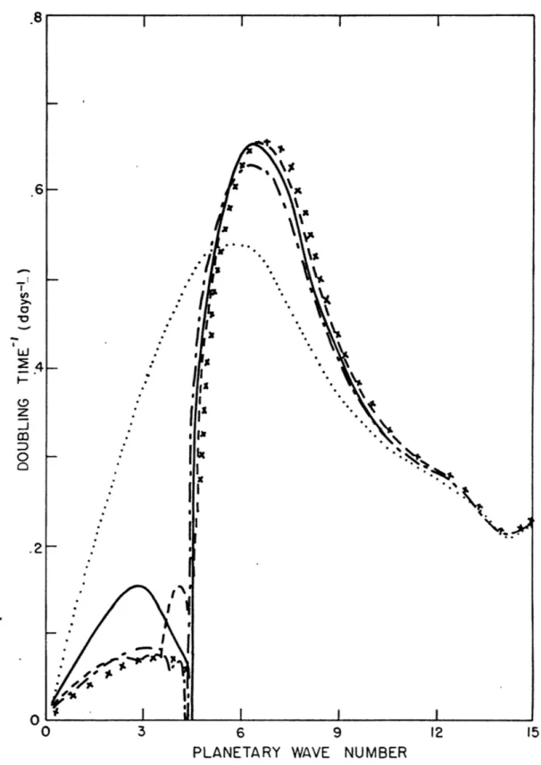
Figures 3.1 to 3.4 present the doubling times and phase velocities of the unstable modes for special and nominal parameter values. It is immediately apparent that the presence or absence of a stratosphere or of the #-effect affects the results much more than variation of the upper layer's shear. The presence of a greater static stability in the upper layer, not surnrisingly, lessens further the influence of upper layer shear variation. Eady modes grow faster for a reversed upper layer shear if no stratosphere is present and very slightly more slowly if there is a strato-sphere. The overall shape of the doubling time curves is little affected

-- -- - 111111~~

by variation of SR. This is not the case for YT. As pointed out by Green (1960), zero A-effect stabilizes short waves. Also, when SR = 1 and there is no stratosphere in addition to no A-effect, all modes are stable; this differs from Green's results for a rigid lid (see discussion of W' = 0 atp=0

calculations). As 'T increases, short waves become more unstable (see

Fig-ures 3.17 and 3.18). The presence of a stratosphere lessens doubling times of the Eady mode for all values of SR and "T from about 2 1/2 to 1 1/2

days. When both the stratosphere and a-effect are present, the long wave "Green Mode appears and has its fastest doubling time (6 days) for the nominal, reversed stratospheric shear. The doubling time and wave number of the most unstable Green and Eady modes for the parameter values CT', SR, Op = 2, 1,

50 compare well with those calculated by Geisler and Garcia (1977) for a constant shear and more realistic temperature profile. Differences are less than 10%.

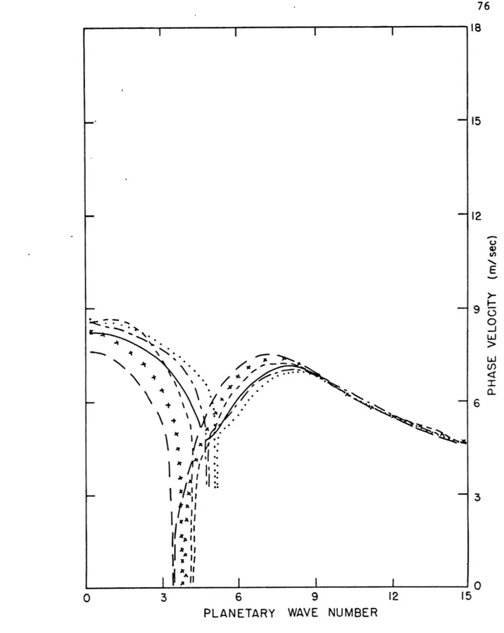
Phase velocities calculated by Geisler and Garcia are almost twice as large as this model's values for T, SR, f = 2, i, 50. The difference

is due to the much larger u values in the former model. A fairer compari-son between this model and that of Geisler and Garcia will be made in the next chapter. For zero 6-effect, phase velocities are very large at long wavelengths (note the change of scale in Figures 3.1 and 3.2). When there

is both a 4-effect and a stratosphere present, the phase velocity goes to zero with the growth rate at a "critical" wavelength which defines the

separation between the Eady and Green modes. The existence of neutral waves stationary relative to the surface wind at this critical wavelength was dis-covered by Green (1960). Steering levels, as in Green's study are below the mid level (p/p = 1/2) for all wavelengths.

-Iu,

Streamfunction amplitudes and phases are presented for the most un-stable Eady and Green Modes in Figures 3.5 to 3.8. For the Eady mode, the presence of a stratosphere causes a sharp peak in YI at the tropopause independent of 8-effect and shear variation. This peak is approximately equal to the peak at the ground. The latter is narrower for YT 0; this also was observed by Green (1960). Variation in SR has negligible effect when 50, but when hen = larger values of MIP occur around the tropo-pause as SR goes to negative values (Figures 3.6 and 3.7). The Green mode, existing only for T 0, o 1 has a strong peak in the stratosphere which moves up from 180 mb to 120 mb as the stratospheric shear reverses.

Streamfunction phases are constant throughout the upper layer when YT = 0 or o = i1. When there is both a p-effect and a stratosphere, the pressure wave tilts westward with height in the stratosphere for both Eady and Green modes, the Green mode having a much greater tilt. In the tropo-sphere the Green mode also has a greater westward tilt.

For quasi-geostrophic disturbances, a westward tilt of the wave with height means entropy is transported poleward (Lorenz, 1951). The model

calculations of v'&' , Figures 3.9 to 3.12, illustrate this property for the fastest growing Eady and Green modes: all tilts are westward and all v' ' values are positive. When there is no d-effect v'9' is independent of 0 and SR values and is zero in the upper layer, reflecting the

con-stancy of phase there. In the presence of both a stratosphere and a B-effect, entropy transports are significant in the stratosphere, for both modes. The Green mode has a much stronger stratospheric transport. It peaks at the tropopause and remains large in the lower stratosphere. The

flux is strongest for the case of reversed shear. Thus, nominal conditions produce modes which have larger stratospheric heat transports than all the other cases considered.

A local maximum in the entropy flux in the lower stratosphere is observed (Oort and Rasmusson, 1971; Newell et al., 1974). Thus, the Green mode could be very important.for lower stratospheric dynamics. This problem will be addressed in more detail in the next chapter.

Except for the Green mode with uniform shear (SR = 1), no modes have kinetic energy generated in the upper layer (see Figures 3.13 to 3.16). Only this Green mode and an Eady mode with no stratosphere and SR = 1

have their kinetic energy destroyed in any region of the lower layer. In all cases there is, of course, a net generation of mode kinetic energy when the entire model atmosphere is considered. And in all cases, there is a net mode kinetic energy generation in the troposphere and net loss in the stratosphere. The maximum mode kinetic energy generation is in the mid to low troposphere for all cases except the Green mode with reversed strato-spheric shear. This latter mode has its strongest kinetic energy genera-tion in the upper troposphere.

Earlier discussion pointed out that for no stratosphere and uniform shear there was apparently no Green mode for YT = 0 or 2, and there were no unstable modes for SR = 1, (7 = 1 and YT = 0. Is there a Green mode for a

stronger effect? What happens to it for small #? These questions are answered by a graph (Figure 3.17) similar to Green's (1960) figure 3 with the difference that Green's rigid lid is replaced byf' = 0 at p = 0* * Differences between this graph and Green's Figure 3 are discussed with the = 0' 0 at p = 0 calculation later in this chapter.

40 The Green mode is seen to exist for large 8-effect (or small tropospheric shear, u ) but is very weak, and its wavelength becomes infinite as yT or

q = 8 _{goes to zero. Also, as yT or q goes to zero, growth rate per unit} YT remains constant so that the growth rate approaches zero with yT or q .

When SR and _{have their nominal values, and}

rT

_{varies, the} situ-ation is much different (see Figure 3.18). The fastest growing Eady mode growth rate changes little as

ycE~r~

to zero, and the Green mode is much stronger and is at a shorter wavelength for IT < 10.

3.5 _{Results for variation of one parameter with others fixed at nominal} values

In this section two parameters are held at their nominal values and the third varies over a wide range of parameter space. Doubling times and phase velocities are obtained for zonal wave numbers 0 to 15, and vertical structures of wave properties are presented for the fastest growing Green and Eady modes. _{Shorter modes are trapped near the ground and are outside} the stratospheric focus of this thesis (Chapter IV illustrates properties of these waves for realistic T and U profiles).

Figures 3.19 to 3.21 show that the doubling time of the fastest growing Green mode is much more sensitive to parameter variation than is the doubling time of the fastest growing Eady mode. The wave numbers of the most unstable Green and Eady modes are not very sensitive to the vari-ation of SR and

0

but increase markedly as T increases. This increase of most unstable mode wavenumber with YT was pointed out earlier (see Figures

3.17 and 3.18). _{As SR takes on values from -12 to 4, the Green mode} re-mains constant in strength for reversed shear in the stratosphere but

be-comes much weaker for large positive SR. The Eady mode, however, bebe-comes slightly stronger and the wavelength for which it is most unstable slightly

increases with SR throughout its range. For values of

0-

between 1 and 1000, the Green mode has its fastest doubling time, 6 days, near the nomi-nal value, = 50 (intermediate calculations, not shown, refines this value of a to be 60). As yT varies from 0 to 10 there is a dramatic de-crease in the Green mode's fastest doubling time - from 12 days (IT = 1)

to 3 days (YT = 10). The wavenumber of the fastest growing Green mode increases from 2.0 to 7.5. Thus, at high

YT

the Green mode is no longer long-wave. Green (1960) has shown that longer waves are expected to have longer doubling times because they only weakly satisfy the necessary con-dition for instability, viz., that particle paths have an average slope between that of the isentropes and the horizontal. -Green's heuristic

argu-ment was for rigid lids at top and bottom. To the extent that a 50-fold increase in the static stability approximates a rigid lid, one can say that the Green mode grows slower at lower

(T

when ~'= 0 in the upper boun-dary conditions because it is at a longer wavelength.

The phase velocities, shown in Figures 3.22 to 3.24, all haveasharp minimum at .the wavenumber which, by definition, separates the Green and Eady modes. The Green mode is defined to include all wavenumbers less than that of the sharp minimum in the phase velocity. There are other, weaker minima in some of the phase velocity curves. These are found to be asso-ciated with weak minima (which may not be resolved) in the doubling time curves. Phase velocities are most strongly influenced by changes in 'fT For all wavelengths, phase velocities decrease with increasing T. And, for all wavenumbers and parameter combinations of this section (except SR

< -2), the unstable modes have a single steering level in the lower tropo-sphere. For a strongly reversed stratospheric shear (SR < -2) some modes have an additional steering level in the stratosphere.

Streamfunction amplitudes and phases for the fastest growing Eady and Green modes are presented in Figures 3.25 to 3.36. The structure of the Eady mode amplitude in the troposphere is little affected by varying SR and a- (except when .' = 1). Peaks of the pressure amplitude occur at the ground and tropopause. The peaks are of approximately equal value and the one at the tropopause decays less rapidly into the stratosphere for small - , when y = 10. When )T begins to increase beyond 3, the tropo-pause peak begins to weaken substantially. Stratospheric Eady mode

pres-sure amplitudes are largest when yT is near its nominal value.

The Green mode has larger streamfunction amplitudes in the strato-sphere than the Eady mode for all parameter combinations of this section. Figures 3.8 and 3.28 through 3.30 show that the Green mode's amplitude peaks

higher in the stratosphere, and has larger values there (relative to those of other levels) when the parameters are near their nominal values. The peak, for near nominal parameter values, occurs at 120 mb, and the ampli-tude remains greater than half the peak value from below the troponause to 30 mb. For YT

A

7, there are pressure amplitude peaks at the tropopause and 75 mb which are separated by a sharp minimum at 140 mb (see Figure 3.30). The upper peak is weaker and has a value of .7 times the tropopause peak value. The Green mode also has a peak at the ground which is as strong as the peak in the stratosphere when 4 10 or SR - -4. In comparison with that of the Eady mode, the vertical structure of the Green mode's pressure

--amplitude is much more sensitive to variations of SR orO . The same was seen to be true regarding the doubling times of the Eady and Green modes, and, as subsequent figures illustrate, the same is also true for the ver-tical structure of mode phase, meridional entropy transport and kinetic energy generation. The larger amplitude of the Green mode at stratospheric levels renders it more sensitive to variations of SR and

0

, which are really variations in the stratospheric shear and static stability because YT is held constant.

The phase of the Eady mode streamfunction varies much less with height than does the phase of the Green mode (Figures 3.31 to 3.36).

Ex-cept for the case of a very stable stratosphere, > 1000, the Eady mode

pressure wave has only a slight westward tilt with height. The tilt of the Green mode is very strongly westward with height and is most strongly west-ward when YT or C are large or when SR = -4. The Green mode has its most

rapid vertical phase variation concentrated in a region just above the tropopause (100-250 mb) and in the lower troposphere (550-750 mb). The phase can change 1800 in these regions. The Green mode and, at a slower

rate, the Eady mode vertical wavelength approaches zero in the stratosphere as ---30 0. Amplitudes of both modes also approach zero in the

strato-sphere as -- 0>cand are negligible for 0 > 1000.

The meridional entropy transports, v'O', of both modes (Figures 3.37 to 3.42) are all poleward, as expected for quasi-geostrophic waves which tilt westward with height. The stratospheric transports are generally very weak for the Eady mode (in comparison to the tropospheric transports) except when the stratospheric shear is easterly (SR < 0), but even these

_ _ _ _ _ _ _ IIIIIu I _ _ _ _ _ l III WIIIII1W 161

transports are far shallower than those of the Green mode in the lower stratosphere. Tropospheric Eady mode v'&' values are little affected by changes in SR and 6, but as YT increases, they decrease rapidly at all levels except near the ground. The entropy transports of the Green mode in the lower stratosphere are generally stronger than those in the tropo-sphere except for transports near the ground when SR is positive,@

,

< 10,

or y 7. The stratospheric Green mode fluxes are countergradient and are T

strongest when the parameters are near their normal values. They have their strongest peak at the tropopause and remain at greater than half the peak value up to 130 mb. Stratospheric Green mode v'O' values are weakest for SR positive or 0 5< 10.

The generation of mode kinetic energy for both Eady and Green modes occurs only in the troposphere except for the Green mode when SR > 0 (see Figures 3.43 to 3.48). In this unique case there is a weak, shallow region above the tropopause where Green mode kinetic energy is generated. The generation of Eady mode kinetic energy is stronger in the lower and mid-troposphere (except for YT = 10; in this case alone there is a weak destruc-tion of mode kinetic energy in a region of the troposphere). The generation of Eady mode kinetic energy is affected only slightly by variations of SR or 9,; however, the generation decreases rapidly as (T increases. The

generation of Green mode kinetic energy when SR4 0,

5

Z 10, or 'T < 7 is nearly constant throughout the troposphere except near the ground where it goes to zero with o; when SR> 0, p = 10, or (T >- 7, there is a mid-tropospheric destruction of Green mode kinetic energy. The strongest Green mode kinetic energy generation is always in the lower troposphere. In

summary, the strongest generation of both Eady and Green mode kinetic energy -

-is in the troposphere. Therefore, both modes are tropospheric in origin. They drive the stratosphere, i.e. they lose kinetic energy in that region and build up zonal available potential energy there with counter-gradient entropy fluxes when SR< 0. The Green mode has much stronger and deeper stratospheric entropy transports and kinetic energy losses in comparison to its tropospheric values of these quantities than does the Eady mode.

It is also a (zonally) longer wave mode and can, according to Gall (1976) more easily penetrate into the stratosphere. Therefore, the Green mode could be of much greater importance to lower stratospheric dynamics than the Eady mode.

3.6 Results for constant YT planes in parameter snace

This section explores a much wider expanse of parameter space. It focuses on the growth rate of the most unstable Eadv and Green modes and discusses properties of their vertical structure which may be of importance to the general circulation at specific levels of the atmosphere. It also ascertains whether any new modes appear in the range of parameter space which it covers. Parameter space of this model has 4 dimensions

represen-ted by

(T,

SR, Gp, and P. The value of the wavenumber P is always chosen to be that of a local maximum in the curve of growth rate vs P. The re-maining 3 dimensions are sampled by examining planes of constant

YT

at

YT

= .5, 2, and 6. On these planes, ' varies from 1 to 1000 and SR varies from 14 or 0 to -14, depending on the value of YT and the mode presented.

The doubling time of the fastest growing Eady mode is contoured on the constant YT planes in Figures 3.49 to 3.51. On all planes there is only a slight variation of doubling time with SR-and CT when r > 20; and

46

the variation is even slighter for larger Y . Most doubling times are be-* tween 1.5 and 2.0 days. There is a lengthening of doubling time to 3 or 4 days for small

a

and ISRI > 10. As seen in the previous section, wavenum-bers of the most unstable Eady mode increase with Y . When YT is not large, * they also increase as

ap

approaches 1 and SR becomes large and negative.

When 0 > 20 they vary little with SR and

a

. The wavenumber will typically double from SR=-2 to SR=-10 (p = 2, y = .5or 2) ; it will also double from

a

a

=50to r =2 (SR=-14, y = .5 or 2) with the most rapid increase at the

P p T

smallest values of

a

. On the YT= 2 plane, the most unstable wavenumber is between 6 and 7 for a > 20 and is near 15 for SR < -8 and

a

< 2.

The fastest-growing Green mode undergoes a much less smooth variation of doubling time with SR and

a

(Figures 3.52 to 3.54). It is much shorter for higher YT , independent of the values of SR and Cp. On all the YT planes, the fastest doubling times are when

ap

is small and SR is large and negative; this is the same region where the Eady mode is weakest. The longest doubling times occur for small

a

and SR going positive. For YT = .5 or 2 there is a region of shorter doubling times for nominal and larger values of a and SR near -2. The nominal point (SR= -1.5, 9p = 50, YT = 2) occurs in a local region of shorter doubling times whose values are about 6 days. The YT = 2 plane shows the most complicated variation of Green mode doubling time with SR and

a

. This, in part, could be due to the difficulty in defining a fastest growing Green mode when there is no minimum of growth rate between the Green and Eady modes

(see the SR = -4 curve in Figure 3.19). In this case, a point .6 zonal wave-numbers to the left of the point of greatest curvature was chosen to be the wavenumber of the fastest growing Green mode (e.g. 3.6 was chosen as the wavenumber of the fastest growing Green mode on the SR= -4 curveof Figure

eNo

..- AUNM 00111WI 111011111MIN 1