Computational Sequence Design Techniques for DNA Microarray Technologies

Publisher’s version / Version de l'éditeur:

Systematic Approaches in Bioinformatics and Computational Systems Biology:

Recent Advances, 2011-07-01

READ THESE TERMS AND CONDITIONS CAREFULLY BEFORE USING THIS WEBSITE.

https://nrc-publications.canada.ca/eng/copyright

Vous avez des questions? Nous pouvons vous aider. Pour communiquer directement avec un auteur, consultez la première page de la revue dans laquelle son article a été publié afin de trouver ses coordonnées. Si vous n’arrivez pas à les repérer, communiquez avec nous à PublicationsArchive-ArchivesPublications@nrc-cnrc.gc.ca.

Questions? Contact the NRC Publications Archive team at

PublicationsArchive-ArchivesPublications@nrc-cnrc.gc.ca. If you wish to email the authors directly, please see the first page of the publication for their contact information.

NRC Publications Archive

Archives des publications du CNRC

For the publisher’s version, please access the DOI link below./ Pour consulter la version de l’éditeur, utilisez le lien DOI ci-dessous.

https://doi.org/10.4018/978-1-61350-435-2.ch003

Access and use of this website and the material on it are subject to the Terms and Conditions set forth at

Computational Sequence Design Techniques for DNA Microarray

Technologies

Tulpan, Dan; Ghiggi, Anthos; Montemanni, Roberto

https://publications-cnrc.canada.ca/fra/droits

L’accès à ce site Web et l’utilisation de son contenu sont assujettis aux conditions présentées dans le site LISEZ CES CONDITIONS ATTENTIVEMENT AVANT D’UTILISER CE SITE WEB.

NRC Publications Record / Notice d'Archives des publications de CNRC:

https://nrc-publications.canada.ca/eng/view/object/?id=63fcb134-6145-4d1f-b1bc-a10ac6ac7a19 https://publications-cnrc.canada.ca/fra/voir/objet/?id=63fcb134-6145-4d1f-b1bc-a10ac6ac7a19

1

Computational Sequence Design Techniques for DNA Microarray

Technologies

Dan Tulpan1, Athos Ghiggi2, Roberto Montemanni3

1 _{Institute for Information Technology, National Research Council of Canada, 100 des Aboiteaux St., Moncton, New} Brunswick, E1A7R1, Canada.

2

Faculty of Informatics, University of Lugano (USI), Via Giuseppe Buffi 13, CH-6904 Lugano, Switzerland. 3_{Istituto Dalle Molle di Studi sull‘Intelligenza Artificiale (IDSIA), Galleria 2, CH-6928}

Manno-Lugano, Switzerland.

Abstract

In systems biology and biomedical research, microarray technology is a method of choice that enables the complete quantitative and qualitative ascertainment of gene expression patterns for whole genomes. The selection of high quality oligonucleotide sequences that behave consistently across multiple experiments is a key step in the design, fabrication and experimental performance of DNA microarrays. The aim of this chapter is to outline recent algorithmic developments in microarray probe design, evaluate existing probe sequences used in commercial arrays, and suggest methodologies that have the potential to improve on existing design techniques.

Introduction

The design of DNA oligos is a key step in the manufacturing process of modern microarrays – biotechnology tools that allow the parallel qualification and quantification of large numbers of genes. Areas that have benefited from the use of microarrays include gene discovery (Andrews et al., 2000; Yano, Imai, Shimizu, and Hanashita, 2006), disease diagnosis (Yoo, Choi, Lee, and Yoo, 2009), species identification (Pasquer, Pelludat, Duffy, and Frey, 2010; Teletchea1, Bernillon, Duffraisse, Laudet, and Hänni, 2008) and toxico-genomics (Jang, Nde, Toghrol, and Bentley, 2008; Neumanna and Galvez, 2002).

Microarrays consist of plastic or glass slides, to which a large number of short DNA sequences (probes) are affixed at known positions in a matrix pattern. A probe is a relatively short DNA sequence (20-70 bases) representing the complement of a contiguous sequence of bases from a target that acts as its fingerprint. The purpose of each probe is to uniquely identify and bind a target via a process called hybridization. Nevertheless, in practice probes could bind to more than one target via a process called cross-hybridization.

While microarrays could be used for a variety of applications like transcription factor binding site identification (Hanlon & Lieb, 2004), eukaryotic DNA replication (MacAlpine & Bell, 2005), and array comparative genomics hybridization (Pinkel & Albertson, 2005), their main use remains gene transcript expression profiling (Schena, Shalon, Davis, & Brown, 1995; Ross et al., 2000; Aarhus, Helland, Lund-Johansen, Wester & Knappskog, 2010). However, at present, the fundamental understandings of the bio-chemo-physical mechanisms that power this technology are poorly understood (Pozhitkov, Tautz, and Noble, 2007), thus leading to hybridization signal levels that are still not accurately correlated with exact amounts of target transcripts. While most of the microarray research work carried today focuses on the development of reliable and fault-tolerant statistical techniques that could pre-process large data sets (Holloway, van Laar, Tothill, & Bowtell, 2002; Irizarry et al., 2003; Quackenbush, 2002; Yang et al., 2002; Zhao, Li, & Simon, 2005) and identify significant factors relevant to each particular study (Chu, Ghahramani, Falciani, & Wild, 2005; Harris & Ghaffari, 2008; Leung & Hung, 2010; Peng, Li, & Liu, 2007; Zou, Yang, & Zhu, 2006), more work needs to be done on improving the infrastructural aspects of microarray technology, thus reducing the amount of noise earlier rather than later in an experiment based on microarrays data.

Thus, one of the greatest challenges in DNA microarray design resides in how to select large sets of unique probes that distinguish among specific sequences from complex samples consisting of thousands of closely similar targets. The daunting task of designing such large sets of probes is hampered by the computational costs associated with probe efficacy evaluations. Various design strategies are presented that employ the utilization of intricate probe evaluation criteria. Some of these strategies were inspired from design techniques employed for solving similar problems that arise in coding theory (Bogdanova, Brouwer, Kapralov, & Östergård, 2001; Gaborit & King, 2005; Gamal, Hemachandra,

2

Shperling, & Wei, 1987), bio-molecular computing (Feldkamp, Banzhaf, & Rauhe, 2000; Frutos et al., 1997), molecular tagging (Braich et al., 2003; Brenner & Lerner, 1992) and nano-structure design (Reif, Labean, & Seeman, 2001; Yurke, Turberfield, Mills, Simmel, & Neumann, 2000).

In recent years there has been considerable interest in the application of meta-heuristic algorithms for the design of DNA strands to be used in microarray technologies. Most of the proposed algorithms deal with combinatorial constraints only (Frutos et al., 1997; Marathe, Condon, & Corn, 2001; Kobayashi, Kondo, & Arita, 2003), in order to increase the tractability of the problem from a computational point of view. On the other hand, because of this simplification, the strands obtained do not always have the desired characteristics when used in experimental settings. Therefore, thermodynamic constraints are typically employed to have satisfactory results in practice, notwithstanding they tend to destroy most of the combinatorial structures exploited by the algorithms themselves. A summary of state-of-the-art combinatorial algorithms is presented here. We then describe how two algorithms originally developed for combinatorial constraints can be extended to efficiently deal with thermodynamic constraints.

The first approach is a Stochastic Local Search method originally described in (Tulpan, Hoos, & Condon, 2002; Tulpan & Hoos, 2003; Tulpan, 2006), which works on the search space of infeasible solutions. This means it starts with a given number of random strands, violating many constraints. There is a fitness measure estimating the severity of the total constraints violation of the solution. The algorithm iteratively modifies the strands with the target of improving the fitness. In the end, if all the constraints are fulfilled, a feasible solution has been found; otherwise the minimal set of strings causing violations can be deleted in order to have a feasible solution.

The second approach analyzed is a Seed Building procedure, originally described in (Montemanni & Smith, 2008; Montemanni & Smith, 2009a; Ghiggi, 2010). Differently from the Stochastic Local Search, this method works on the space of feasible solutions: it starts from an empty set of strands and iteratively enlarges it with strands, which are feasible with those already added to the set. From time to time the set is partially destroyed in order to diversify the search.

De-novo experimental results are presented for the two meta-heuristic algorithms discussed. Based on a set of combinatorial and thermodynamic criteria presented in literature, we present a case study including the evaluation of existing probe sets used in Affymetrix microarrays where probe and target sequence information is publicly available. Analyses of such sets provide insights on their strengths and weaknesses and also shed light on potential areas of improvement that can only empower the existing technologies thus increasing their impact in the specific areas of applicability. For example, high throughput similarity searches performed on Affymetrix probe sets of Human Gene arrays and the most recent gene sequence information available in public databases (NCBI, Ensembl) reveal that close to 5-10% of the probes used on some arrays are either not unique or they do not identify the correct target (Wang et al., 2007). Here, we present further evidence, that a careful re-analysis and re-consideration of the microarray probe design techniques for different microarrays should be explored in greater detail.

Related Work

A large number of computational probe design techniques (see Table 1) have been developed over the past 15 years and their impact on the microarray-based experimental results is massive. A number of review papers (Kreil, Russell, & Russell, 2006; Lemoine, Combes, & Le Crom, 2009) collect and describe the particular features of each package, including the set of constraints used for probe design, their versatility, usability and availability.

Software Reference URL Status

ARB (Ludwig et al., 2004) http://www.arb-home.de/ WD

Array Designer 4.25 (Premier Biosoft) http://www.softpedia.com/get/Science-CAD/Array-Designer.shtml WD

ArrayOligoSelector (Bozdech et al., 2003) http://arrayoligosel.sourceforge.net/ WD

ChipD (Dufour et al., 2010) http://chipd.uwbacter.org/ CS

CommOligo v2.0 (Li, Hel, & Zhou, 2005) http://ieg.ou.edu/software.htm WD

Featurama/ProbePicker (ProbePicker) http://probepicker.sourceforge.net/ NA

GenomePRIDE v1.0 (Haas et al., 2003) http://pride.molgen.mpg.de/genomepride.html FA

3

Software Reference URL Status

HPD (Chung et al., 2005) http://brcapp.kribb.re.kr/HPD/ NA

MPrime (Rouchka, Khalyfa, & Cooper, 2005) http://kbrin.a-bldg.louisville.edu/Tools/MPrime/ CS

OliCheck (Charbonnier et al., 2005) http://www.genomic.ch/download.php WD

Olid (Talla, Tekaia, Brino, & Dujon, 2003) NA FA

OligoArray v2 (Rouillard, Zuker, & Gulari, 2003) http://berry.engin.umich.edu/oligoarray2/ WD

OligoDb (Mrowka, Schuchhardt, & Gille, 2002) http://bioinf.charite.de/oligodb/ CS

OligoDesign (Tolstrup et al., 2003) http://oligo.lnatools.com/expression/ CS

OligoFaktory (Schretter & Milinkovitch, 2006) http://oligofaktory.lanevol.org/index.jsp FA

OligoPicker (Wang & Seed, 2003) http://pga.mgh.harvard.edu/oligopicker/ WD

OligoSpawn (Zheng et al., 2006) http://oligospawn.ucr.edu/ NA

OligoWiz (Nielsen, Wernersson, & Knudsen, 2003) http://www.cbs.dtu.dk/services/OligoWiz/ WD, CS

Oliz (Chen & Sharp, 2002) http://www.utmem.edu/pharmacology/otherlinks/oliz.html NA

Osprey (Gordon & Sensen, 2004) http://osprey.ucalgary.ca/cgi-bin/oligo_array CS

PICKY (Chou, Hsia, Mooney, & Schnable, 2004) http://www.complex.iastate.edu/download/Picky/index.html WD

PrimeArray (Raddatz, Dehio, Meyer, & Dehio, 2001) http://pages.unibas.ch/wtt/Products/PrimeArray/primearray.html FA

PRIMEGENS v2 (Srivastava, Guo, Shi, & Xu, 2008) http://compbio.ornl.gov/structure/primegens/ NA

ProbeMaker (Stenberg, Nilsson, & Landegren, 2005) http://probemaker.sourceforge.net/ WD

Probemer (Emrich, Lowe, & Delcher, 2003) http://probemer.cs.loyola.edu/ NA

Probe-sel (Kaderali & Schliep, 2002) NA FA

ProbeSelect (Li & Stormo, 2001) http://ural.wustl.edu/resources.html NA

ProbeWiz (Nielsen & Knudsen, 2002) http://www.cbs.dtu.dk/services/DNAarray/probewiz.php CS

ProMide (Rahmann, 2003) http://oligos.molgen.mpg.de/ FA

ROSO (Reymond et al., 2004) http://pbil.univ-lyon1.fr/roso/ CS, NA

SEPON (Hornshoj, Stengaard, Panitz, & Bendixen, 2004) http://www.agrsci.dk/hag/sepon/ NA

Teolenn (Jourdren et al., 2010) http://transcriptome.ens.fr/teolenn/ WD

SLSDNADesigner (Tulpan et al., 2005) http://www.cs.ubc.ca/labs/beta/Software/DnaCodeDesign/ WD

YODA (Nordberg, 2005) http://pathport.vbi.vt.edu/YODA/ NA

Table 1: A selection of popular probe design software packages and their availability as of August 2010. The acronyms used in this table have the following meaning: WD = web download, NA = not available (web site), FA = from authors,

CS = client-server

From a software design perspective, typically, probe design applications can be grouped into two categories: (i) client-server applications, and (ii) autonomous software.

Client-server software

The client-server category is well represented by a series of software packages like ChipD (Dufour et al., 2010), FastPCR (Kalendar, Lee, & Schulman, 2009), Gene2Oligo (Rouillard, Lee, Truan, Gao, Zhou, et al., 2004), MPrime (Rouchka, Khalyfa, & Cooper, 2005), OligoDB (Mrowka, Schuchhardt, & Gille, 2002), OligoDesign (Tolstrup et al., 2003), OligoWiz (Nielsen, Wernersson, & Knudsen, 2003), Osprey (Gordon & Sensen, 2004), ProbeWiz (Nielsen & Knudsen, 2002) and ROSO (Reymond et al., 2004) that use various algorithmic techniques and constraint combinations. Due to the computational speed and information transfer limitations via web services, many of these applications are optimized for speed, thus the selection of criteria used for probe design tend to be more combinatorial, heuristic and empirical in nature.

One of the latest software, ChipD (Dufour et al., 2010), is a new probe design web server that facilitates the design of oligos for high-density tilling arrays. The software relies on an algorithm that optimizes probe selection by assigning scores based on three criteria, namely specificity, thermodynamic uniformity and uniform coverage of the genome. OligoDesign (Tolstrup et al., 2003) provides optimal locked nucleic acid (LNA) probes for gene expression profiling. As a first step, the software reduces probe cross-hybridization effects by employing a genome-wide BLAST analysis

4

against a given set of targets. Next, each probe gets assigned a combined fuzzy logic score based on melting temperature, self-annealing and secondary structure for LNA oligos and targets. At the end, the highest ranking probe is reported.

OligoWiz (Nielsen, Wernersson, & Knudsen, 2003) selects probes based on a set of five criteria: specificity, melting temperature, position within transcripts, sequence complexity and base composition. A score is assigned for each criterion per probe and a weighted score is computed. The probes with the best scores are further selected and visualized in a graphical interface.

Osprey (Gordon & Sensen, 2004) designs oligonucleotides for microarrays and DNA sequencing and incorporates a set of algorithmic and methodological novelties including hardware acceleration, parallel computations, position-specific scoring matrices, which are combined with a series of filters including melting temperature, dimer potential, hairpin potential and secondary (non-specific) binding.

ProbeWiz (Nielsen & Knudsen, 2002) is a probe design client-server application that relies on a two stage approach. In the first stage, the input sequences (FASTA or GenBank accession numbers) are locally aligned with BLAST (Altschul, Gish, Miller, Myers, & Lipman, 1990) against a selected database and the result is filtered using melting temperature, dimer potential, hairpin potential and secondary (non-specific) binding. The second stage optimizes the input obtained in the previous stage by applying a set of filters including probe length, melting temperature, 3‘ proximity, a probe quality score obtained with PRIMER3 (Rozen & Skaletsky, 2000) and a paralogy score.

ROSO (Reymond et al., 2004) consists of a suite of 5 probe selection steps. First, it filters out all input sequences that are identical and masks also the repeated bases within them. The second step consists of a similarity search using BLAST. Next step consists of eliminating probes that self-hybridize. The fourth step eliminates all probes that have undesired melting temperatures. The last step selects a final set of probes based on four additional criteria: GC content, first and last bases, base repetitions and self-hybridization free energies.

Autonomous software

The autonomous software category includes a wider variety of programs that allows the user to have more control over the platform where the application is installed and run, while permitting in the same time the usage of larger input files and better control of the configuration parameters.

OliCheck (Charbonnier et al., 2005) is a program designed to test the validity of potential microarray probes by considering the possibility of cross-hybridization with non-target coding sequences. This analysis can be performed within a single genome or between several different strains/organisms.

OligoArray (Rouillard, Herbert, & Zuker, 2002) takes into account the following criteria: specificity, position within transcript, melting temperature, self hybridization and presence of specific subsequences in the probe. The algorithm runs as follows: it selects a probe starting from the end of the first sequence in the input data set and checks it against all the aforementioned criteria. If the probe satisfies all criteria, the algorithm moves to the next input sequence; otherwise it selects a new probe after a 10 base jump towards the 5‘ end of the input sequence. The process continues until a probe that satisfies all criteria is found. If no such probe is found, the algorithm selects a probe that has a lower probability for cross hybridization. The second version of OligoArray (Rouillard, Zuker, & Gulari, 2003) introduces thermodynamic constraints in the design of oligos.

The ProbeSelect (Li & Stormo, 2001) algorithm is centered on the specificity of sequences and consists of seven steps. First, the program builds a suffix array for the input sequences, to quickly identify the high similarity regions in the input sequences. Then, the algorithm builds a landscape for each input sequence. A landscape represents the frequency in the suffix array of all subsequences in the query input sequence. The third step consists in selecting a list with 10 to 20 candidate probes for each input sequence that minimizes the sum of the frequencies of their subsequences in the suffix array. The fourth step consists in searching for potential cross-hybridizations between each probe and the set of input sequences. Step 5 marks the cross-hybridizations within the input sequences. The next step consists of melting temperature and self-hybridization free energy computations for each remaining probe. The last step consists in selecting the probes, which have the most stable perfect-match free energy and hybridize the least with all the other potential targets.

Some autonomous oligonucleotides design programs are implemented in scripting languages like Perl or Python and are usually much slower than those implemented in C++. OligoPicker (Wang & Seed, 2003) is a Perl program, which also

5

uses a traditional approach. The criteria taken into account are specificity (use of BLAST), melting temperature and position in the transcripts. ProMide (Rahmann, 2003) consists of a set of Perl scripts, with a C program for basic calculations, which uses the longest common substring as a specificity measure for the oligonucleotides. It uses complex data structures such as ‗enhanced suffix array‘ and some statistical properties of sequences. Oliz (Chen & Sharp, 2002) is also implemented in Perl and uses a classical approach relying on BLAST for specificity testing. It however requires additional software to function, like cap3, clustalw, EMBOSS ―prima‖ and a database in the UniGene format. The originality of the method stems from the fact that the oligonucleotides are searched in the 3‘ untranslated region of the mRNAs, a very specific area where sequences are largely available through expressed sequence tag projects.

The majority of the client-server and autonomous software described above use a pipelined filtering approach for the design of microarray probes, where at an initial stage a local alignment approach is employed for cross-hybridization avoidance and then each ulterior filter evaluates the quality of each probe and ranks them according to well defined scoring criteria.

DNA SEQUENCE DESIGN - PROBLEM DESCRIPTION

A single stranded DNA molecule is a long, unbranched polymer composed of only four types of subunits. These subunits are the deoxyribonucleotides containing the bases adenine (A), cytosine (C), guanine (G) and thymine (T). The nucleotides are linked together by chemical bonds and they are attached to a sugar-phosphate chain like four kinds of beads strung on a necklace (Figure 1). The sugar-phosphate chain is composed by alternating the ribose and phosphate for each nucleotide. This alternating structure gives each base and implicitly the whole strand a direction from the ribose end (denoted by 5‘) to the phosphate end (denoted by 3‘). When the 5‘/3‘ ends are not explicitly labeled, DNA sequences are assumed to be written in 5‘ to 3‘ direction.

Figure 1: Idealized structure of a pair of hybridized DNA sequences.

The nucleotides composing DNA bind to each other in pairs via hydrogen bonds in a process known as hybridization. Each nucleotide pairs up with its unique complement (the Watson-Crick complement), so C pairs up with G and A with T. C and G pair up in a more stable manner than A and T do, which is due to one extra hydrogen bond in the C-G pair. The Watson-Crick complement of a DNA strand is the strand obtained by replacing each C nucleotide with a G and vice versa, and each T nucleotide with an A and vice versa, and also switching the 5‘ and 3‘ ends. For example the Watson-Crick complement of 5‘-AACTAG-3‘ is 3‘-TTGATC-5‘. Non-Watson-Crick base pairings are also possible. For example, G-T pairs occur naturally in biological sequences (Ho et al., 1985; Pfaff et al., 2008).

Formally, these notions are captured in the following definitions:

A DNA strand w is represented by a string over the quaternary alphabet {A, C, G, T}. String w corresponds to a single-stranded DNA molecule with the left end of the string corresponding to the 5‘-end of the DNA strand.

The complement, or Watson-Crick complement, of a DNA strand w is obtained by reversing w and then by replacing each A with a T and vice versa, and replacing each C in the strand by G and vice versa. We denote the Watson-Crick complement of a DNA strand w with c(w) and we will simply use the terms complementary strand, or complement in this work. For simplicity, we simply use ci instead of c(wi).

Throughout the remainder of the chapter we use symbols w1, w2, ..., wk to denote unique strands and c1, c2, ..., ck to

C

A

G

T

3’

5’

C

A

G

T

3’

_5’

6

denote the corresponding complements. Thus, strand wi and complement ci form a perfect match (duplex), whereas strand wi and complement cj, and complements ci and cj, with j ≠ i, form mismatches. We will call probes the strands attached to the surface of microarrays, while targets are the corresponding complements floating in the solution. We adopt this terminology because it is widely used in the literature on DNA microarrays.

Finally, we formalize the optimization version of the DNA Strand Design Problem.

The DNA Strand Design (DSD) Problem is defined as follows: with respect to a fixed set C of constraints (which are part of the input and will be detailed in the reminder of the section), given a strand length n, find the largest possible set S with DNA strands of length n, satisfying all the constraints in C.

The constraints used in the design of DNA strands can be grouped into two classes: combinatorial and thermodynamic constraints. The grouping is based on the measures that estimate the quality of one or more DNA strands upon which the constraint is applied. Combinatorial constraints mostly rely on verifying the presence or absence of certain nucleotides in a strand, and counting of matches and/or mismatches for pairs of DNA strands, whereas thermodynamic constraints take into account the biochemical properties that govern DNA hybridization.

COMBINATORIAL CONSTRAINTS

Combinatorial constraints are widely used to design large sets of non-interacting DNA strands. The necessity of designing sets of strands that avoid cross-hybridization can be superficially modeled by enforcing a high number of mismatches between all possible pairs of strands and between pairs of strands and the complements of others. The stability and uniformity of DNA strands can be also modeled with combinatorial constraints by either controlling the presence or absence of undesired subsequences or counting specific bases within the same strand. Various types of combinatorial constraints can be considered. In the following paragraphs we will formalize those of interest for our study.

C1: Direct Mismatches. The number of mismatches in a perfect alignment of two strands (also referred to as Hamming distance) must be above a given threshold d. Here, a perfect alignment is a pairing of bases from the two strands, where the ith _{base of the first strand is paired with the i}th _{base of the second strand, and a mismatch is a pairing of} two distinct bases. For example, G paired with A, C, or T is a mismatch whereas G paired with G is a match. For example, the strands w=5‘-AACAA-3‘ and wI=5‘-AAGAA-3‘ have one mismatch at position i = 3, where i = 1, 2, …, 5.

C2: Complement Mismatches. The number of mismatches in a perfect alignment of a strand and a complement must

be above a given threshold d. For example, the complement of strand w=5‘-AACAA-3‘, which is c=5‘-TTGTT-3‘ and strand wI=5‘-TTATT-c=5‘-TTGTT-3‘ have one mismatch at position i = 3, where i = 1, 2, …, 5. This constraint is also referred to as the reverse-complement constraint.

C3: GC Content. The number of G‘s and/or C‘s in a strand must be in a given range. For example, all strands

presented in (Braich et al., 2003) have 4, 5 or 6 C‘s. One such strand is w=5‘-TTACACCAATCTCTT-3‘, which contains five Cs.

Constraint C3 can be used to attain desired hybridization. Roughly, the stability of a strand-complement pair increases as the content of G‘s and C‘s within strands increases. Constraint C3 is also used to ensure uniform melting temperatures across desired strand-complement pairings. Constraints C1 and C2 can be used in various combinations to avoid undesired hybridization. As it is widely known, the strength of hybridization between two strands (or between bases of the same strand) depends roughly on the number of nucleotide bonds formed (longer perfectly paired regions are more stable than shorter ones; this is modeled by C1 and C2), and on the types of nucleotides involved in bonding. It can be observed that checking if a combinatorial constraint is satisfied can be done with computational complexity O(n). This makes these constraints extremely tractable from a computational point of view.

THERMODYNAMIC CONSTRAINTS

7

applications, their lack of accuracy is well known. More accurate measures of hybridization are required to efficiently predict the interaction between DNA strands. A higher level of accuracy can be achieved by understanding the thermodynamic laws that govern the interaction between bases of DNA strands. Thermodynamic constraints have been defined and used to design high quality sets of DNA strands.

Before presenting the thermodynamic constraints necessary to obtain such sets, it is necessary to provide a brief introduction to the underlining thermodynamic principles that govern DNA strand interactions.

With the primary goal of predicting secondary structure and DNA / RNA stability from the base sequence, over the past 20 years a number of melting temperature and diffraction based studies have been conducted to estimate the relationship between thermodynamic stability and DNA base sequences, in terms of nearest-neighbor base pair interactions.

The nearest-neighbor (NN) model for nucleic acids was pioneered in the 1960s by (Crothers & Zimm, 1964) and by (Devoe & Tinoco, 1962). Subsequently, several papers and theoretical reports on DNA and RNA nearest-neighbour thermodynamics have been published. In 1986, Breslauer et al. reported a first set of nearest-neighbor sequence-dependent stability parameters for DNA obtained from evaluation of melting curves of short DNA oligomers (Brelauer, Frank, Blöcher, & Marky, 1986). Following that study, further research in the field lead to the development of more complex and accurate sets of DNA and RNA parameters (Gotoh & Tagashira, 1981; Vologodskii, Amirikyan, Lyubchenko, & Frank-Kamenetskii, 1984; Delcourt & Blake, 1991; Doktycz, Goldstein, Paner, Gallo, & Benight, 1992; SantaLucia, Allawi, & Seneviratne, 1996; Sugimoto, Nakano, Yoneyama, & Honda, 1996; SantaLucia, 1998; Tulpan, Andronescu, & Leger, 2010).

Free energies are always lower or equal with zero for any pair of DNA strands. The lower the free energy is for a DNA duplex, the more stable the duplex is.

In this chapter, we use the PairFold program implemented by Mirela Andronescu to compute free energies for DNA duplexes (Andronescu, 2003; Andronescu, 2008). The PairFold program predicts the secondary structure of a pair of DNA molecules based on free energy minimization. The secondary structure for a pair of strands (w, w I) is a set of base pairs, with each base of w and wI occurring in at most one pair. PairFold returns four secondary structures, for the pairs (w, wI), (wI, w), (w, w), and (wI, wI), and their corresponding minimum free energies. The algorithm uses dynamic programming and runs in time bounded by the cube of the lengths of the input strands. A detailed view of the computational model used in this work, which takes into consideration complex interactions between DNA sequences, can be found in (Andronescu, Zhang & Condon, 2005).

Thermodynamic constraints rely on the thermodynamic nearest-neighbor model presented above. We use the DNA parameters of SantaLucia Jr. (SantaLucia, 1998) (a set of unpublished parameters have been previously obtained via private communication with John SantaLucia) and PairFold to calculate minimum free energies of duplexes. We use the parameters and Equation (3) of (SantaLucia & Hicks, 2004) to calculate melting temperatures, assuming a 1M salt concentration and 1e−07 M concentration of both strands and complements (for a total concentration of 2 x 1e-07 M). The melting temperature is only calculated for perfectly matched duplexes. Throughout, we use the following notation: T denotes the temperature of the reaction, R = 1.98717 kcal/(mol · K) is the gas constant, ∆G0 (x, y) is the minimum free energy of the duplex xy at standard conditions (room temperature of 24 oC and absolute pressure of 1 atm), and TMi denotes the melting temperature of strand wi.

In this chapter we will consider the following thermodynamic constraints:

T1: Complement Mismatch Free Energy. The free energy of a strand and the complement of a distinct strand must be in a given range. For example, the complement mismatch free energy range of the strands in the set S=

{TTTAAA, AAAAAA} is [—1.04, —0.33] kcal/mol.

T2: Complement-Complement Mismatch Free Energy. The free energy of a complement-complement duplex must

be in a given range. For example, the complement-complement mismatch free energy range of the strands in the set S ={AATTCC, GGCCAA, TTCCGG} is [—1.86, —0.81] kcal/mol.

Constraints T1 and T2 are used to restrict undesired hybridization, which can occur between a strand and the complement of a different strand (T1), or between two distinct complements (T2). In the context of microarrays, constraint T2 is the most important one. Constraint T1 is also marginally important although usually not applied against

8

all the possible strand complements.

With respect to combinatorial constraints, checking thermodynamic constraints is more demanding from a computational point of view, since checking a constraint takes up to O(n3

) (free energy has to be computed each time).

STATE OF THE ART OF HEURISTIC ALGORITHMS

There has been considerable interest recently in the application of meta-heuristic algorithms to the DSD problem. Most of the works appeared so far in the literature consider a simplified version of the problem, where only some combinatorial constraints are considered, while the more realistic constraints coming from the thermodynamic interactions among strands are neglected. The choice of not considering these latter constraints come from the consideration that they tend to break the combinatorial structure of the problem, on which most of the methods developed so far were actually based. When only combinatorial constraints are considered, bounds for the size of DNA codes can be obtained by generalizing classic results coming from algebraic coding theory, template-map strategies, genetic algorithms and lexicographic searches (Chee & Ling, 2008; Deaton et al., 1996; Deaton, Murphy, Garzon, Franceschetti, & Stevens, 1999; Faulhammer, Cukras, Lipton, & Landweber, 2000; Frutos et al., 1997; Gaborit & King, 2005; King, 2003; Li, Lee, Condon, & Corn, 2002; Smith, Aboluion, Montemanni, & Perkins; Zhang & Shin, 1998). In (Tulpan et al., 2002) and (Tulpan et al., 2003) a Stochastic Local Search method, able to handle large problems has been developed. In (Montemanni et al., 2008) four new local search algorithms were developed and combined into a variable neighborhood search framework, following ideas originally developed in (Montemanni et al., 2009a) for constant weight binary codes. Further results are presented in (Montemanni & Smith, 2009b), (Montemanni, Smith, & Koul) and (Koul, 2010), where a new simulated annealing procedure and an evolutionary algorithm are discussed. Other interesting algorithms worth to be mentioned are (the list is not comprehensive): a method based on ant colony optimization discussed in (Ibrahim, Kurniawan, Khalid, Sudin, & Khalid, 2009) and (Kurniawan, Khalid, Ibrahim, Khalid, & Middendorf, 2008); a global search approach presented in (Kai, Z., Linqiang & Jin, 2007); a randomized algorithm proposed in (Kao, Sanghi, & Schweller, 2009); a particle swarm optimization method discussed in (Khalid, Ibrahim, Kurniawan, Khalid, & Enggelbrecht, 2009).

Only a few algorithms have been presented to handle thermodynamic constraints. These methods are pure meta-heuristic approaches, and connections with coding theory are weaker, since the combinatorial structures of the instances tend to be destroyed by these constraints. They also face intrinsic computational difficulties due to the necessity of calculating free energies (a time consuming task) many times during the execution. The stochastic local search algorithm discussed in (Tulpan et al., 2002) and (Tulpan et al., 2003) is extended to handle thermodynamic constraints in (Tulpan et al., 2005) and (Tulpan, 2006), where results are presented. In (Ghiggi, 2010) one of the local searches originally presented in (Montemanni et al., 2008) - Seed Building - is modified to handle these constraints. These last two algorithms will be detailed and experimentally compared on some test instances in the next sections.

STOCHASTIC LOCAL SEARCH

Stochastic local search (SLS) algorithms strongly use randomized decisions while searching for solutions to a given problem. They play an increasingly important role for solving hard combinatorial problems from various domains of Artificial Intelligence and Operations Research, such as satisfiability, constraint satisfaction, planning, scheduling, and other application areas (Hoos & Stützle, 2004). Over the past years there has been considerable success in developing SLS algorithms as well as randomized systematic search methods for solving these problems, and to date, stochastic local search algorithms are amongst the best known techniques for solving problems from many domains. In particular, SLS methods are indicated for complex problems, for which a model cannot be directly used to devise solutions. The DSD problem with thermodynamic constraints lies in this category.

The stochastic local search algorithm introduced by Tulpan et al. in 2002 (Tulpan, Hoos, & Condon, 2002) performs a randomized iterative improvement search in the space of DNA strand sets. All strand sets constructed during the search process have exactly the target number of strands. It is ensured that all strands in the given candidate set always have the prescribed GC content. The proposed SLS algorithm starts with a target number of strands k and attempts to minimize the number of pairs that violate the given constraint(s). After all the constraint violations have been eliminated, or a given maximum computation time has elapsed, the algorithm stops. In the latter case a post-processing phase has to be run in order to eliminate the smallest possible number of strands, leading to the largest possible residual feasible set of strands. A pseudo-code for the overall algorithm is as follows:

9

StochasticLocalSearch()

Input: number of strings (k), string length (n), set of combinatorial constraints (C) Output: set S of m strings that satisfy constraints C

For i := 1 to maxTries do S := initial set of strings S’ := S

For j := 1 to maxSteps do

If (S satisfies all constraints) then return S

Randomly select strings w1, w2 S that violate at least one of the constraints M1 := all strings obtained from w1 by substituting one base

M2 := all strings obtained from w2 by substituting one base With probability θ do

Select string w’ from M1 M2 at random Otherwise

Select string w’ from M1 M2 such that the number of conflicts is maximally decreased If (w’ M1) then

Replace w1 by w’ S Otherwise

Replace w2 by w’ S

If (S has no more constraint violations than S’) then S’ := S

Return S’

The initial set of k strands is determined by a simple randomized procedure that generates any DNA strand of length n fulfilling GC content constraints with equal probability. Note that the initial strand set may contain multiple copies of the same strand.

A loop is then entered. At each step of the search process, first, a pair of strands violating one of the constraints (either combinatorial or thermodynamics) is selected uniformly at random. Then, for each of these strands, all possible single-base modifications complying with the required GC content are considered. As an example of single-base modifications, consider the strand ACGT of length 4. A new strand TCGT can be obtained by replacing letter A from the first strand with letter T. With a given probability θ, one of these modifications is accepted uniformly at random, regardless of the number of constraint violations that will result from it. In the remaining case (with probability 1 — θ), each modification is assigned a score, defined as the net decrease in the number of constraint violations caused by it, and a modification with maximal score is accepted. If there are multiple such modifications, one of them is chosen uniformly at random. Note that using this scheme, in each step of the algorithm, exactly one base in one strand is modified.

The parameter θ, also called the noise parameter, controls the greediness of the search process; for high values of θ, constraint violations are not resolved efficiently, while for low values of θ, the search has more difficulties to escape from local optima of the underlying search space. Throughout the run of the algorithm, the best candidate solution encountered so far, i.e., the DNA strand set with the fewest number of constraint violations, is memorized. Since the algorithm evolves a set of infeasible strings trying to reduce a measure of infeasibility, we say that it works in the infeasible search space. If the algorithm terminates without finding a valid set of size k, a valid subset can always be obtained by applying the following post-optimization phase. The algorithm builds a graph and then solves a maximum clique problem, where the maximum clique corresponds to the largest possible set of mutually feasible strands. The method is detailed in the remainder of this section.

MAXIMUM CLIQUE POST-OPTIMIZATION

A maximum-clique post-optimization algorithm was introduced by Ghiggi in 2010 (Ghiggi, 2010). The first stage of the algorithm consists of constructing a graph G = {V, E} as follows. The set V corresponds to the strands retrieved (k in this case). An edge {i, j} ∈ E exists if no constraint violation exists between the strands associated with nodes i and j. An example of such a graph can be found in Figure 2.

10

Figure 2: Example of maximum clique problem. The largest maximum clique has size 4 and is the subgraph consisting

of vertices 2, 4, 5 and 6.

After having built the graph as described above, the problem of retrieving the largest possible set of strands mutually fulfilling combinatorial and thermodynamic constraints is equivalent to solving a maximum clique problem on the graph G. In graph theory a maximum clique of a graph G is defined as the largest complete subgraph of G, where complete means that an edge must exist between each pair of vertices of the subgraph (Pardalos & Xue, 1994). In this case, finding a complete subgraph means to look for a subset of strands mutually fulfilling all the constraints, thus we look for the largest possible subset.

The advantage of the problem transformation described above is that very efficient algorithms exist to solve the maximum clique problem. The implementation used in this work adopts the algorithm cliquer (Östergård, 2002).

SEED BUILDING

Algorithms that examine all possible strands in a given order, and incrementally accept strands that are feasible with respect to already accepted ones, can often produce fairly good codes when only combinatorial constraints are considered (Gaborit & King, 2005; King, 2003; Montemanni et al., 2009a; Montemanni, Smith, & Koul). For this reason the Seed Building (SB) method is based on these orderings, combined with the concept of seed strands (Brouwer, Shearer, Sloane, & Smith, 1990). These seed strands are an initial set of strands with the required GC-content and feasible with respect to each other, to which strands are added in the given ordering if they satisfy the necessary criteria. In our implementation we generate strands in a random order. Preliminary experiments suggested that, in contrast to binary codes (Montemanni et al., 2009a), a random order is preferable for DNA codes (Montemanni, Smith, & Koul). In this section we describe how a Seed Building strategy can be modified to deal with thermodynamic constraints, too (Ghiggi, 2010).

Seeds can be selected at random, but experiments on binary codes and on DNA code design problems with combinatorial constraints only, clearly show that there is a better way to proceed: in the seed building algorithm a set of seeds is initially empty, and one random seed (feasible with respect to the previous seeds, and fulfilling the GC-content constraint) is added at a time. If this seed leads to good results, it is kept, and a new random seed is designated for testing, thus increasing the size of the seed set. The same rationale is used to decide whether to keep subsequent seeds or not. In the same way, if after a given number of iterations the quality of the solutions

11

provided by a set of seeds is judged to be not good enough, the most recent seed is eliminated from the set, which results therefore in a reduction in the size of the seed set. In this way the set of seeds is expanded or contracted depending on the quality of the solutions provided by the set itself. What happens in practice is that the size of the seed set oscillates through a range of small values.

A pseudo-code for the algorithm is the following one:

SeedBuilding()

Input: maximum time (TimeSB), maximum number of iterations with the same set of seeds (ItrSeed), set of combinatorial constraints (C)

Output: set S of strings that satisfy constraints C Seeds := Ø

S := Ø ItrCnt := 0

While (Computation time < TimeSB) do ItrCnt := ItrCnt + 1

Cstring := random string with proper GC content, compatible with Seeds WordSol := Seeds {Cstring}

Complete WorkSol by adding feasible strings examined in a random order If (|WorkSol| > |S|)

ItrCnt := 0 S := WorkSol

Seeds := Seeds {CString} // Added in the last position If (ItrCnt == ItrSeed)

AclSeed := average code size in the last ItrCnt iterations AclAll := average code size from the beginning

If (AclSeed >AclAll)

CString := random string with proper GC content compatible with Seeds Seeds := Seeds {CString} // Added in the last position

Else

If (|Seeds| > 0)

CString := String in the last position of Seeds Seeds := Seeds \ {CString}

ItrCnt := 0 Return S

The Seed Building algorithm works in an iterative fashion on an adaptive set of seed strands contained in the set SeedSet, which is initially empty. At each iteration, a new strand CString, compatible with those in Seeds, is generated and the partial solution WorkSol, initialized with the elements of Seeds and CString, is expanded by adding feasible strands, examined in a random order. If a new best solution is found, the set Seeds is immediately expanded. Every ItrSeed iterations, the average size of the codes generated with the set Seeds is checked to determine whether Seeds is a promising set (in which case it should be augmented) or not (in which case it is reduced by deleting the most recently added seed). The procedure stops after a fixed computation time of TimeSB seconds has elapsed.

Preliminary tests clearly suggested (Ghiggi, 2010) that applying the general Seed Building paradigm when dealing with thermodynamic constraints is computationally intractable with current technology: too many time-consuming free energy evaluations would be necessary, leading to a method able to perform just a few iterations in an affordable computation time. This suggested that SB is probably less indicated than SLS to deal with thermodynamic constraints. However, it is possible to implement a workaround able to make SB applicable to problems with thermodynamic constraints. In order to explore the solution space in a satisfactory way, we need to minimize the number of free energy evaluations necessary to understand whether the various constraints are violated or not. In our implementation, we compute only one special case of thermodynamic constraint T2 at each iteration, while we postpone the evaluation of the remaining one into a post-optimization phase. This permits to reduce the number of free energy computations, focusing on those that show to be crucial in shaping up the solutions. The resulting algorithm can be therefore sketched as follows:

1. Processing phase: classic Seed Building algorithm where combinatorial constraints are considered together with a special case of the T2 constraint. Here each string is only checked against itself, but not against the strands already in

12

the solution. The hope is that this particular T2 constraint is sufficient to filter out most of the unfeasible strands, and to shape up the solution in an efficient way.

2. Post Processing phase: starting from the solution obtained in the previous point, a graph is built analogously to what was done before for the Stochastic Local Search approach. At this point we know that all combinatorial constraints and self-T2 are fulfilled, so we need to take care only of the residual T2 thermodynamic constraints. Notice that the number of free energy evaluations is of the order of O(s2

), where s is the number of strands produced at phase 1. This number is intuitively small if the filter provided in phase 1 is efficient. Again analogously to what was done before, it is sufficient now to run a maximum clique algorithm to retrieve the largest possible clique in the graph, which corresponds to a feasible solution for the original problem.

Even when the two phase approach is adopted, we can say that the SB algorithm works in the feasible search space, in the sense that it only produces feasible solutions (according to the constraints considered in phase 1), that are incrementally increased during the computation. This is the main difference with respect to the Stochastic Local Search method described above.

It is important to emphasize that the decomposition described above is not based on any theoretical results guarantying optimality: it is a heuristic criterion that might lead to suboptimal solutions. Everything basically depends on the filter provided by phase 1. Experimental results discussed in the next section clearly suggest that the decomposition approach is effective in practice.

COMPUTATIONAL EXPERIMENTS

In this section we compare the results obtained by the two meta-heuristic methods described in the previous sections.

EXPERIMENTS SET UP

The comparison between the two algorithms is based on the number of feasible strands retrieved at the end of the computation. Since SLS requires the target number of strands k as input, we provide SLS with k = res(SB); k = res(SB)*1.1 and k = res(SB)*1.2, where res(SB) is the number of feasible strands retrieved by seed building. In this way we check whether SLS is able to replicate, or improve the results of SB. Notice that the final result returned by SLS is less than or equal to k by definition, since infeasible strands are deleted in the post-optimization phase, as described in the previous section. In order to run experiments, we also have to define feasible free energy values for the thermodynamic constraints T1 and T2. We used the values calculated empirically and reported in (Ghiggi, 2010), which are reported in Figure 3. Notice that the same thresholds have been used for all the thermodynamic constraints considered. The parameter settings used for the algorithms are those reported in (Ghiggi, 2010), where we refer the interested reader for the details.

The other parameter settings used for the algorithms are those reported in (Ghiggi, 2010): for the SLS algorithm probability θ = 0.2, MaxTries = 10 and MaxSteps = 50000; ItrSeed = 5 and TimeSB = 600 seconds for the SB algorithm.

Figure 3: Feasible free energy ranges for constraints T1 and T2.

Results

Theoretical results

In Figure 4 the results obtained by the different algorithms while considering constraints C1, C2, C3 and T2 are reported. For different values of n (measuring the length of the strands) and of d (the threshold for the distance involved in combinatorial constraints C1 and C2) the results of the Stochastic Local Search algorithm, on the left of each cell, and those of the Seed Building method, on the right, are reported. Notice that for the Stochastic Local Search algorithm the best results among the different values of k considered are reported, with a superscript indicating the configuration that generated the result of each cell. Notice that some of the entries are missing (-) since the corresponding test was not run.

13

Figure 4: Computational results obtained for constraints C1, C2, C3 and T2

From Figure 4 it emerges that SLS is better in the quasi-diagonal part of the table (i.e. right below the diagonal corresponding to n=d), while SB has to be preferred otherwise. The result can be explained by observing that SLS searches in the infeasible search space, making it possible to modify strands, while SB incrementally accepts strands at each iteration (feasible search space). This makes difficult to find optimal solutions for those settings where only a few combinations of strands are optimal.

As previously observed, in the context of microarrays, the thermodynamic constraint of major interest is T2, nevertheless constraint T1 plays a role, too. For this reason we run some tests of the algorithms we propose also on the combination of constraints C1, C2, C3, T2 and T1. Results are reported in Table 2, where some combinations of n and d values are considered. Notice that for the Stochastic Local Search algorithm the best results among the different values of k considered (the same used for Figure 4) are reported, this time without indicating the configuration that generated the result of each entry.

A comparison of Figure 4 and Table 2 suggests that the introduction of constraint T1 substantially decreases the dimension of the feasible sets of strands. Future research will investigate the reasons for this phenomenon.

14

n d SB SLS 12 6 27 13 12 7 9 8 12 8 3 5 12 9 2 2 13 8 5 6 13 9 2 2 13 10 2 2 14 7 34 10 14 8 12 6 14 9 6 5 14 10 2 2 14 11 2 2 15 9 4 3 15 10 2 1 15 11 1 1 16 9 8 3 16 10 5 2 16 11 2 2 17 9 2 1 18 10 9 3 19 11 12 3 19 12 3 2 20 13 2 2 20 14 2 2

Table 2: Computational results obtained for constraints C1, C2, C3, T2 and T1

Case study: Computational evaluation of Affymetrix probe sequences

Over the past 15 years Affymetrix microarrays constituted one of the most widely used experimental platforms for gene expression studies. Each array consists of a solid wafer (quartz substrate) to which large numbers of 25mer probes are attached. Gene expression levels are measured by hybridizing mRNA extracted from cells or tissues of interest to the probes on the array. For each expressed transcript Affymetrix assigns one or more probe sets, each consisting of 11-20 series of probe pairs. Each pair consists of one perfect match probe and one mismatch probe. The perfect match probe corresponds to the complementary sequence of the gene of interest, while the imperfect match probe has the middle nucleotide at position 13 replaced by its Watson-Crick complement.

The array design process employed by Affymetrix technology for Gene Arrays typically includes a series of successive steps, as follows:

- Large numbers of sequences and annotations are collected from publicly available databases including NCBI RefSeq, GenBank and dbEST.

- The sequences are aligned to genome assemblies for each organism and their quality and orientation is evaluated based on consensus splice sites, known polyadenylation sites and confirmed coding sequences.

15

Here we consider the case study where industrially produced microarray probes are evaluated in-silico based on 74 out of a total of 86 publicly available probe and target sequence data sets made available by Affymetrix Corporation, Santa Clara, CA. The remaining 12 out of 86 array data was incomplete, meaning that either probe or target sequences (but not both) were available on the NetAffx web site. The species covered by Affymetrix microarray technology span a wide taxonomic range including the realms of plants, amphibians, bacteria, birds, fungi, insects, mammals (mouse and human included) and worms. The total number of complete (probe, target) sequence sets made available by Affymetrix for their arrays are 18,460,805 and respectively, 1,492,049. While Affymetrix technology makes use of perfect match and mismatch probe sequences, this study will only analyze the perfect match probes.

Affymetrix Probe and Target Sequence Characteristics

As one of the biggest producers of microarrays in the world, Affymetrix uses a technology employing multiple synthesized oligonucleotide probes, each one being 25 nucleotides long, to identify and discriminate among large numbers of targets. The data analyzed in this chapter shows that the Affymetrix array with the highest number of distinct probe sequences is the Wheat array (674,353 probes), while the array that tests the highest number of targets is the Poplar array (61,413 targets). The lowest number of probe sequences can be found in the RT-U34 rat array (20,464 probes). The lowest number of targets corresponds to the same rat RT-U34 array (1,031 targets).

The following indicators were used for the evaluation of the probe design quality of the Affymetrix arrays: - Number of duplicate probe and target sequences,

- Probe sequence homology with NCBI RefSeq and Affymetrix target sequences,

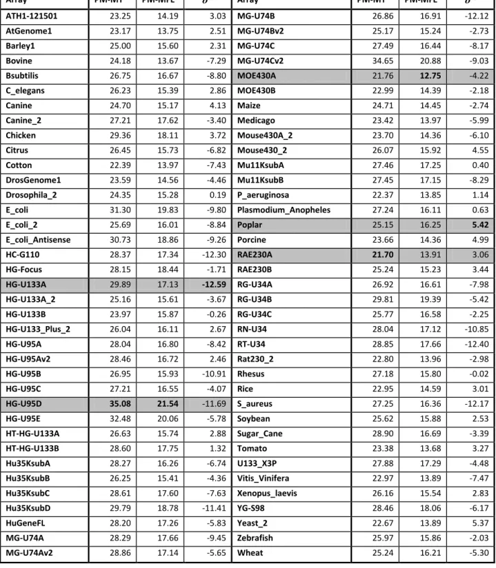
- Thermodynamic evaluation of probe sequences: melting temperatures, perfect match minimum free energies, GC-content.

Each one of these indicators can be used to gauge the quality of the probe sequences or the overall quality of a microarray.

Sequence duplication

The presence of identical probe sequences on a microarray will affect the specificity of those probes and will diminish the signal strength since the same target, if present, could potentially bind to all locations where the given probe is present. A close analysis of the Affymetrix probe sequences (see Table 3) reveals that only those designed for the P.aeruginosa array bear no duplications, the remaining 73 arrays containing up to 9.47 % (11,696 / 123,524) probe duplication for the S.aureus array. A similar analysis of the Affymetrix targets shows one potential cause of the probe duplication problem, namely that only 7 out of 74 arrays have no duplicated targets. The remaining 67 arrays show up to 1.55 % (16 / 1031) target sequence duplication for the rat array RT-U34.

Array Num probes Num Dup Probes % Num targets Num Dup Targets %

ATH1-121501 251,078 212 0.08 22,814 0 0.00 AtGenome1 131,822 894 0.68 8,297 15 0.18 Barley1 251,437 2,575 1.02 22,840 60 0.26 Bovine 265,627 690 0.26 24,128 4 0.02 Bsubtilis 100,584 51 0.05 5,039 9 0.18 C_elegans 249,165 2,987 1.20 22,625 2 0.01 Canine_2 473,162 3,345 0.71 43,035 56 0.13 Canine 263,234 1,254 0.48 23,913 13 0.05 Chicken 424,097 1,879 0.44 38,535 26 0.07 Citrus 341,730 5,269 1.54 30,372 123 0.40

16

Array Num probes Num Dup Probes % Num targets Num Dup Targets %

Cotton 265,516 1,719 0.65 24,132 30 0.12 DrosGenome1 195,994 112 0.06 14,010 1 0.01 Drosophila_2 265,400 481 0.18 18,955 15 0.08 E_coli_2 112,488 108 0.10 10,208 2 0.02 E_coli_Antisense 141,629 547 0.39 7,140 9 0.13 E_coli 141,629 547 0.39 7,312 9 0.12 HC-G110 30,313 19 0.06 1,887 15 0.79 HG-Focus 98,149 339 0.35 8,793 0 0.00 HG-U133A_2 247,899 6,062 2.45 22,283 0 0.00 HG-U133A 247,965 6,067 2.45 22,283 0 0.00 HG-U133B 249,502 977 0.39 22,645 0 0.00 HG-U133_Plus_2 604,258 9,726 1.61 54,675 47 0.09 HG-U95A 201,807 1,717 0.85 12,454 15 0.12 HG-U95Av2 201,800 1,727 0.86 12,453 15 0.12 HG-U95B 201,862 2,671 1.32 12,620 24 0.19 HG-U95C 201,867 1,376 0.68 12,646 16 0.13 HG-U95D 201,858 584 0.29 12,644 16 0.13 HG-U95E 201,863 851 0.42 12,639 17 0.13 HT-HG-U133A 247,719 6,058 2.45 22,268 0 0.00 HT-HG-U133B 249,453 972 0.39 22,665 25 0.11 Hu35KsubA 140,010 59 0.04 8,934 16 0.18 Hu35KsubB 139,996 16 0.01 8,924 15 0.17 Hu35KsubC 140,008 107 0.08 8,928 15 0.17 Hu35KsubD 139,985 254 0.18 8,928 16 0.18 HuGeneFL 131,541 200 0.15 6,633 20 0.30 MG-U74A 201,964 1,121 0.56 12,654 16 0.13 MG-U74Av2 197,993 956 0.48 12,488 16 0.13 MG-U74B 201,960 446 0.22 12,636 15 0.12 MG-U74Bv2 197,131 160 0.08 12,477 15 0.12 MG-U74C 201,963 1,664 0.82 12,728 15 0.12 MG-U74Cv2 182,797 309 0.17 11,934 15 0.13 MOE430A 249,958 4,471 1.79 22,690 18 0.08 MOE430B 248,704 1,505 0.61 22,575 21 0.09 Maize 265,682 4,830 1.82 17,734 44 0.25 Medicago 673,880 8,878 1.32 61,278 167 0.27 Mouse430A_2 249,958 4,471 1.79 22,690 18 0.08 Mouse430_2 496,468 5,978 1.20 45,101 39 0.09 Mu11KsubA 131,280 75 0.06 6,584 15 0.23 Mu11KsubB 119,580 989 0.83 6,002 53 0.88 P_aeruginosa 77,674 0 0.00 5,900 0 0.00 Plasmodium_Anopheles 250,758 4,017 1.60 22,769 149 0.65 Poplar 674,330 11,539 1.71 61,413 280 0.46 Porcine 265,635 519 0.20 24,123 2 0.01 RAE230A 175,477 502 0.29 15,923 5 0.03

17

Array Num probes Num Dup Probes % Num targets Num Dup Targets %

RAE230B 168,984 479 0.28 15,333 4 0.03 RG-U34A 140,317 260 0.19 8,799 21 0.24 RG-U34B 140,312 19 0.01 8,791 15 0.17 RG-U34C 140,284 32 0.02 8,789 15 0.17 RN-U34 21,305 5 0.02 1,322 15 1.13 RT-U34 20,464 57 0.28 1,031 16 1.55 Rat230_2 342,410 968 0.28 31,099 9 0.03 Rhesus 668,485 3,801 0.57 52,865 65 0.12 Rice 631,066 17,890 2.83 57,381 352 0.61 S_aureus 123,524 11,696 9.47 7,775 67 0.86 Soybean 671,762 5,343 0.80 61,170 102 0.17 Sugar_Cane 92,384 1,425 1.54 8,387 23 0.27 Tomato 112,528 198 0.18 10,209 2 0.02 U133_X3P 673,904 42,190 6.26 61,359 903 1.47 Vitis_Vinifera 264,387 2,795 1.06 16,602 74 0.45 Xenopus_laevis 249,678 4,143 1.66 15,611 55 0.35 YG-S98 138,412 3,872 2.80 9,335 114 1.22 Yeast_2 120,855 423 0.35 10,928 6 0.05 Zebrafish 249,752 2,282 0.91 15,617 27 0.17 Wheat 674,353 30,278 4.49 61,290 614 1.00 AVG 249,470.34 3,284.30 0.98 20,162.82 54.70 0.25 MAX 67,4353 42,190 9.47 61,413 903 1.55 MIN 20,464 0 0.00 1,031 0 0.00

Table 3: Duplicate probe and target sequences in Affymetrix arrays.

While the use of multiple probes allows Affymetrix technology to better and widely asse ss the expression levels of numerous target genes, we believe the presence of identical probe sequences as components of various probe sets will negatively influence the final outcomes of the microarray experiments, since the expression signals will have shared components that will act as confounders in the final results analysis.

Sequence homology between probes and non-targets

In Affymetrix arrays, all probes within a probe set should ideally estimate the expression level of the same target, since their sequences are specifically designed to uniquely identify it. Nevertheless, high levels of variation for probe intensities, which are consistent across multiple array experiments that use the same platform, have been reported in the literature (Li & Wong, 1998; Cambon, Khalyfa, Cooper, & Thompson, 2007). It was hypothesized that among the multiple causes of variability of probes within a probe set, the most prominent one is their unintended affinity to bind non-targets (cross-hybridization). A number of very specific studies that focused on Affymetrix arrays designed for various species like Rattus Norvegicus (Cambon, Khalyfa, Cooper, & Thompson, 2007), Homo Sapiens (Barnes, Freudenberg, Thompson, Aronow & Pavlidis , 2005; Harbig, Sprinkle, & Enkemann, 2005; Kapur, Jiang, Xing, & Wong, 2008) and Mus Musculus (Yee, Wlaschin, Chuah, Nissom, & Hu, 2008), were carried out to test this hypothesis. Here we report our findings based on a mass homology search of all Affymetrix array-specific complemented probe sequences against their intended Affymetrix targets and NCBI RefSeq coding sequences.

18

When complements of Affymetrix probe sequences are matched against Affymetrix targets in a homology exact match search using BLAST (word size = 25, e-value = 1e-04), in average 88.09% of the probes match exactly one target, while 10.52% match more than one target and 1.39% do not have a match. The only array that shows an unusually high percentage of probes without a match (90.92%) corresponds to the Rat230 Affymetrix array. The same array proves also to be the only one with 0% single matches. The array with the lowest percentage of mismatched probes (0%) is the P.aeruginosa array, while the array with the highest percentage of probes with multiple matches (89.03%) is the E.coli array.

When RefSeq sequences are used as targets in a homology search we notice a drop of the average percentage of probes that match exactly one target (36.75%) as opposed to when Affymetrix targets are considered. The average percentage of probes that do not match any RefSeq target is much higher (46.78%) than in the previous scenario, possibly suggesting that consensus sequences used by Affymetrix at the time when the array probes were designed were different than the ones available today. The average percentage of probes that match more than one target is only 6% higher (16.47%) than in the previous case. We notice again that the highest percentage of probes that do not match any targets corresponds to the same Rat230 array (94.76%), while the array with the lowest percentage (7.64%) is the HG-Focus array. The array with the highest percentage (71.07%) of probes that match exactly one target is the RN-U34 rat array, while the one with the lowest percentage (0.04%) is again the Rat230 array. The array with the highest percentage of probes (35.89%) with multiple hits is the HC-G110 human array, while the one with lowest percentage (1.48%) is the Citrus array.

Array # probes # targets # s_at % _s_at # x_at % _x_at

ATH1-121501 251,078 22,746 10,415 4.15 1,408 0.56 AtGenome1 131,822 8,297 22,826 17.32 0 0.00 Barley1 251,437 22,840 39,709 15.79 11,790 4.69 Bovine 265,627 24,128 2,859 1.08 1,012 0.38 Bsubtilis 100,584 5,039 320 0.32 0 0.00 C_elegans 249,165 22,625 60,561 24.31 13,530 5.43 Canine 263,234 23,913 23,858 9.06 5,968 2.27 Canine_2 473,162 43,035 148,336 31.35 10,764 2.27 Chicken 424,097 38,535 90,893 21.43 5,071 1.20 Citrus 341,730 30,372 78,759 23.05 17,563 5.14 Cotton 265,516 24,132 102,209 38.49 17,212 6.48 DrosGenome1 195,994 14,010 2,464 1.26 0 0.00 Drosophila_2 265,400 18,955 27,823 10.48 1,204 0.45 E_coli 141,629 7,312 0 0.00 0 0.00 E_coli_2 112,488 10,208 79,267 70.47 1,142 1.02 E_coli_Antisense 141,629 7,140 1,025 0.72 0 0.00 HC-G110 30,313 1,887 6,912 22.80 0 0.00 HG-Focus 98,149 8,793 36,301 36.99 4,257 4.34 HG-U133A 247,965 22,283 87,894 35.45 26,719 10.78 HG-U133A_2 247,899 22,283 87,883 35.45 26,708 10.77 HG-U133B 249,502 22,645 27,606 11.06 15,906 6.38 HG-U133_Plus_2 604,258 54,675 124,377 20.58 46,277 7.66 HG-U95A 201,807 12,454 17,984 8.91 0 0.00 HG-U95Av2 201,800 12,453 17,936 8.89 0 0.00 HG-U95B 201,862 12,620 6,480 3.21 0 0.00 HG-U95C 201,867 12,646 7,230 3.58 0 0.00