Autonomous quadrotor unmanned aerial vehicle for culvert inspection

Autonomous Quadrotor Unmanned Aerial Vehicle

for Culvert Inspection

by

Nathan E. Serrano

S.B., Massachusetts Institute of Technology (2010)

Submitted to the Department of Electrical Engineering and Computer Science

in partial fulfillment of the requirements for the degree of

MASSACHUSETS INSTITUTE OF TECHfNOLCW

AUG 2 2 2011

LiBRARIES

RCHIVES

Master of Engineering in Electrical Engineering and Computer Science at the

MASSACHUSETTS INSTITUTE OF TECHNOLOGY June 2011

©

A uthor ... v..- - - -'" ( - .----...

Department of Electrical Engineering and Computer Science May 20. 2011 Certified by ... Seth Teller Professor Thesis SuDervisor Certified by ... Nicholas 2 Associate Professor Thesja-upervisor Certified by... Te 'ical A ccepted by ... Jonathan Williams

Staff, MIT Lincoln Laboratory

Thwsis Supervisor

Dr. Chritpher J. Terman

Autonomous Quadrotor Unmanned Aerial Vehicle for

Culvert Inspection

by

Nathan E. Serrano

Submitted to the Department of Electrical Engineering and Computer Science on May 20, 2011, in partial fulfillment of the

requirements for the degree of

Master of Engineering in Electrical Engineering and Computer Science

Abstract

This document presents work done to lay the foundation for an Unmanned Aerial Vehicle (UAV) system for inspecting culverts. By expanding upon prior progress creating an autonomous indoor quadrotor, many basic hardware and software issues are solved. The main new functionality needed for the culvert inspection task was to utilize the Global Positioning System (GPS) available outdoors to make up for the relative scarcity of objects visible to the Light Detection And Ranging sensor (LIDAR). The GPS data is fused in a new state estimator, which also incorporates data from the scan matcher running on the LIDAR data, as well as the data from the quadrotor's Inertial Measurement Unit (IMU). This data is combined into a single estimate of the current state (position, orientation, velocity, angular velocity, and acceleration) of the quadrotor by an Extended Kalman Filter (EKF). This new state estimate enables autonomous outdoor navigation and operation of this micro-UAV. Thesis Supervisor: Seth Teller

Title: Professor

Thesis Supervisor: Nicholas Roy Title: Associate Professor

Thesis Supervisor: Jonathan Williams

Acknowledgments

I would like to thank all the staff at MIT Lincoln Laboratory who have helped me on

this project. That includes Justin Brooke, Jonathan Williams, and Matthew Cornick, who all gave me valuable time out of their days, as well as the other members of the Advanced Capabilities and Systems Group (Group 107). Professor Nicholas Roy and the Robust Robotics group made this project possible by sharing their platform with me, and offering me assistance on numerous occasions. Abraham "Abe" Bachrach deserves special thanks for all his help with the quadrotor's software. I would also like to thank my thesis supervisor Seth Teller. Of course I would also like to thank my family for their tireless support of me throughout my academic career.

Nathan Edmond Serrano, 2011

This work is sponsored by the Office of the Assistant Secretary of Defense for Research and Engineering ASD(R&E) under Air Force Contract FA8721-05-C-0002. Opinions, interpretations, conclusions and recommendations are those of the author and are not necessarily endorsed by the United States Government.

Contents

2 Quadrotor System Overview 21 2.1 H ardw are . . . . 21

2.1.1 The Quadrotor: The Ascending Technologies Pelican . . . . . 21

2.1.2 The LIDAR: Hokuyo UTM-30LX . . . . 24

2.1.3 Base Station . . . . 25

2.2 Softw are . . . . 25

2.2.1 LCM... ... . . . . . . . . .. 25

2.2.2 Q uad. . . . . . . 25

2.2.3 The Scan Matcher . . . . 27

3 The State Estimator 29 3.1 T he State . . . . 29

3.2 The Data... . . . . . . . . 30

3.2.1 Scan Matcher Data . . . . 30

3.2.2 G PS D ata . . . . 30

3.2.3 IM U D ata . . . . 31

3.3 The System Dynamics . . . . 31 7

3.4 The Extended Kalman Filter. . . . . 32 3.4.1 Noise Parameters . . . . 33 3.5 Implementation . . . . 34 4 Results 37 4.1 Summary of Results . . . . 37 5 Conclusion 45

5.1 Suggestions for Future Work . . . . 45

5.2 Closing Remarks . . . . 45

A Source Code 47

List of Figures

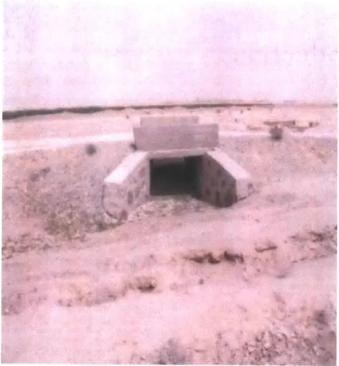
1-1 A culvert typical of those for which routine investigation is required. 16

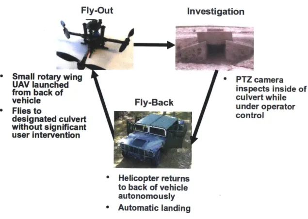
1-2 Mission concept sequence. . . . . 17

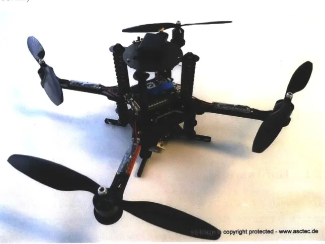
2-1 Image of the Ascending Technologies Pelican . . . . 22

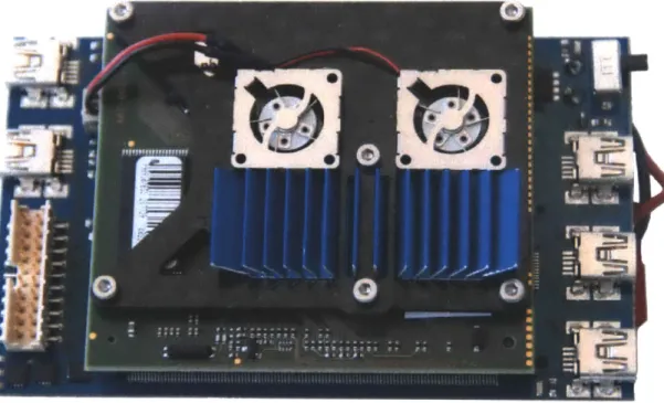
2-2 Image of the Intel Atom-powered Processing Board . . . ... 23

2-3 Image of the Hokuyo UTM-30LX scanning laser range finder. . . . . . 26

2-4 The LIDAR mounted on the quadrotor . . . . 26

2-5 The function of the scan matcher . . . . 28

4-1 Image of the data collection area... . . . . . . . . . 38

4-2 Image of the quadrotor mounted on a cart for data collection. .... 39

4-3 State estimator trial 1: stationary with all sensors . . . . 40

4-4 State estimator trial 2: moving with all sensors . . . . 41

4-5 State estimator trial 3: stationary with no LIDAR . . . . 42

List of Tables

List of Algorithms

Chapter 1

Introduction

1.1

Motivation

MIT Lincoln Laboratory is committed to rapidly developing technological solutions to support the goals of its Department of Defense (DoD) sponsors. One of the DoD's main concerns is always the protection of US servicemen and their allies. Many road-ways within the Central Command Area of Operations (CENTCOM AOO) are raised off of the ground on a dirt berm by about a meter. At frequent intervals, culverts are dug under the road surface to allow for drainage and irrigation (see Figure 1-1). Cul-verts pose a daunting force protection challenge because they are frequently used for explosive emplacement associated with Improvised Explosive Device (IED) attacks.

IED attacks have been a major cause of coalition casualties throughout the wars in

Iraq and Afghanistan. Inspecting culverts is an important, time-consuming, and often dangerous part of counter-IED route clearance patrols. The culvert entrances can be difficult to reach, and while the patrol is stopped it is vulnerable to further attack.

A small Unmanned Aerial Vehicle (UAV), able to be transported and launched by a

small team from the back of a standard HUMVEE, would be able to reach culverts easily while the patrol is at a safe distance and still moving. The key functionality desired for such a system is ease of operation through semi-autonomous operation.

Figure 1-1: A culvert typical of those for which routine investigation is required.

1.2

Mission Concept

A rotary wing UAV has the advantage over a fixed-wing aircraft (in this case) for its

Vertical Take-off and Landing (VTOL) ability which lets it launch and land from a very small area, and to hover outside a culvert while keeping its sensors stable. The solution concept decided on for the present project involves launching and recovering this type of micro-UAV from the back of a military vehicle. The UAV would then

fly to the culvert entrance in question with limited to no input from the operator.

Once outside the culvert, an operator could use a Pan-Tilt-Zoom (PTZ) camera to investigate the culvert. Once satisfied with the inspection of the culvert, the UAV could be told to return to the vehicle autonomously, where it could be readied for the next mission (see Figure 1-2).

Fly-Out Investigation

* Small rotary wing UAV launched from back of vehicle Flies to designated culvert without significant user intervention Fly-Back

/

1.3

Previous Work

The indoor autonomous UAV system developed by Professor Nicholas Roy's Robust Robotics Group was used as a surrogate platform for currently deployed ducted fan military micro-UAVs [1]. It uses a scanning LIDAR and scan matcher to estimate its position, then preforms exploration and Simultaneous Localization and Mapping

(SLAM) in unstructured indoor (GPS-denied) environments . An extended Kalman filter is used to fuse the data from the multiple sensors into one state estimate [2].

Great strides have been made in the control of quadrotors in structured envi-ronments under ideal sensing conditions. The University of Pennsylvania GRASP (General Robotics, Automation, Sensing and Perception) lab has created control al-gorithms for both aggressive maneuvering and cooperative lifting using quadrotors in a motion-capture environment [5].

The Kalman filter was first described in by Kalman in 1960 [4]. It is an optimal estimate of the state of a linear system. When the process to be estimated and/or the relationship of the measurements to that process are non-linear (as it is in all but the simplest robotic systems), the extended Kalman filter is used [8], [9]. The process of using the extended Kalman filter to fuse data from multiple sensors and control a small helicopter has been used on successful systems even before the work done by the Robust Robotics Group [3]. The unscented Kalman filter can give more accurate results than the extended in many circumstances, and has been used successfully for a UAV sensor fusion application, but has a slightly higher computational cost, and is more complex to implement [6].

1.4

Project Overview

The goal of this project was to develop the foundation of an Unmanned Aerial Vehicle

(UAV) system for inspecting culverts. Many basic hardware and software issues

had been solved by previous work, as discussed in the previous section. The main new functionality needed for the culvert inspection task was to utilize the Global

Positioning System (GPS) available outdoors to make up for the relative scarcity of objects visible to the LIDAR. In this project, the GPS data was fused in a new state estimator, which can also incorporate data from the scan matcher running on the LIDAR data, as well as the data from the quadrotor's Inertial Measurement Unit

(IMU). This data is combined into a single estimate of the current state (position

and motion in space) of the quadrotor by an Extended Kalman Filter (EKF). This new state estimator enables autonomous outdoor navigation and operation of this micro-UAV. GPS is not accurate enough to control a micro-UAV alone, and can be easily corrupted further or lost altogether by any structures that introduce multi-path errors or obstruct line-of-sight to the GPS satellites. For this reason, it is essential in all outdoor autonomous robotics to fuse GPS data with other, more accurate sensors to obtain a robust system. The capability of state estimation developed during this work could be of use for many outdoor robotics projects. By changing a handful of constants and coefficients, the filter can be adapted to use data from other sensors, and therefore can be used for a wide variety of systems.

Chapter 2

Quadrotor

System Overview

2.1

Hardware

The hardware portion of the system is made up of the quadrotor (with attached sensors), and the base station computer. Small (under one meter wide) quadro-tors (sometimes referred to as quadrocopters) have gained recent popularity because of the availability of low-cost MEMS-based (microelectromechanical system) IMUs which are required for their construction . Quadrotors have the hovering ability of a helicopter, but are more stable because the two pairs of counter-rotating rotors can-cel out the angular accan-celeration from the motors. Quadrotors are also mechanically simpler than a standard helicopter, as they use fixed-pitch rotors, and maneuver by simply varying the speeds of the rotors individually.

2.1.1

_{The Quadrotor: The Ascending Technologies Pelican}

The Pelican is a quadrotor UAV manufactured and sold by Ascending Technologies GmbH in Krailling, Germany (see Figure 2-1). The Pelican is specifically marketed to-wards academic research applications, where its small size but relatively large payload capacity would be beneficial. It was designed (and in fact, named) in collaboration with Professor Nicholas Roy's Robust Robotics group in the Massachusetts Insti-tute of Technology's (MIT) Computer Science and Artificial Intelligence Laboratory

(CSAIL).

Figure 2-1: Image of the Ascending Technologies Pelican in its off-the-shelf configu-ration.

Specifications

The Pelican has a rotor-tip to rotor-tip size of only 27 inches. In its default con-figuration, the Pelican weighs only 2.869 pounds with its battery. Its four brushless motors can propel it to speeds of 50 km/h and carry a payload of 500 grams. Power is supplied by a lithium polymer (LiPo) battery: 6500 milliampere-hour (mAh) at

11.1 volts.

The Intel Atom Processing Board

One feature that makes the Pelican uniquely suited to autonomy research is the relatively powerful onboard processing board. In addition to the autopilot board that controls the basic stabilization and functions of the quad, the Pelican comes equipped

with a 1.6 GHz Intel Atom processor-powered embedded computer with 1 GB of RAM (see Figure 2-2). Weighing only 90 grams, this computer is powerful enough for all of the computation to be done on-board the vehicle, avoiding communication lag issues. It also contains a Wi-Fi 802.1 In wireless network interface controller (WNIC), allowing high-bandwidth communication.

Figure 2-2: Image of the Intel Atom-powered Processing Board

The Global Positioning System Receiver

The Pelican also comes equipped with a Global Positioning System (GPS) receiver.

GPS is an invaluable navigation tool for outdoor operation. The GPS is made up

of a series of satellites in Low Earth Orbit, which transmit a message that includes the precise time the message was sent, and the exact details of its orbit. Using the messages from four or more satellites, a receiver anywhere on or near the earth can triangulate its position by calculating its distance from each satellite using the time it took the message to reach the receiver. In order to receive the relatively weak signals from the satellites, a system must essentially have unobstructed view of the sky. Under ideal conditions (i.e. unobstructed horizon-to-horizon view), about eight

satellites are visible from any point on the earth at any time. GPS receivers commonly output their current Latitude and Longitude.

The Inertial Measurement Unit

Integral to even the most basic flight operation of the Pelican (and all quadrotors), is the Inertial Measurement Unit (IMU), which consists of a series of MEMS sensors that afford the vehicle perception of its own motion and orientation. The Pelican

IMU includes a three-axis compass and a pressure sensor for altitude measurements.

2.1.2

The LIDAR: Hokuyo UTM-30LX

The Hokuyo UTM-30LX is a lightweight scanning laser range finder or LIDAR (LIght Detection And Ranging) sensor (see Figure 2-3). Scanning LIDARs use a laser, shining on a spinning mirror, to measure distance to a 2-Dimensional arc of their surroundings by precisely measuring the round-trip time of the laser to and from an obstacle. The Hokuyo UTM-30LX scans 270 degrees in front of the sensors, out to a maximum detection range of 30 meters, at 40 scans per second. It offers satisfactory performance at a weight of only 370 grams, allowing it to be used even with the tight size, weight, and power constraints of a micro-UAV. The laser used is classified as a type-1 laser, certifying that it is eye-safe, an important factor for any robot that will be used in close proximity to human operators.

The LIDAR on the Pelican

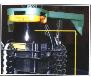
The Hokuyo LIDAR is mounted in the center of the Pelican, above the level of the rotors. Professor Roy's group developed an additional modification to the LIDAR to gain even more data about the quadrotor's surroundings. By adding a new bracket to the top of the LIDAR, mirrors are suspended in the path of the laser redirecting a small portion of the scan vertically, in order to measure the altitude of the quadrotor

(see Figure 2-4). A mirror is positioned on both sides of the LIDAR, at the edge of its scan range, one redirecting the scan down for altitude and one redirecting the

scan up for measuring overhead clearance.

2.1.3

Base Station

The system is tied together by a standard commercial laptop computer running Ubuntu Linux that acts as the base station. Visualization and logging are run on this computer, and it can be used for particularly computationally intensive algorithms (e.g., Simultaneous Localization and Mapping (SLAM)). The laptop is connected to a commercial wireless router, which communicates over IEEE 802.11n Wi-Fi with the computer on-board the UAV.

2.2

Software

2.2.1

LCM

LCM (Lightweight Communication and Marshalling), developed by the MIT DARPA Urban Challenge Team in 2007, is a publish/subscribe architecture where all modules of the robot's software publish data to open channels, and then subscribe to the specific channels necessary for that module. A full description of LCM, including the source code, has been made available on Google Code [7]. LCM is designed for real-time systems, and has the advantage of enforcing modularity, while simultaneously enabling transparency and debugging. As all messages can be viewed and recorded

by another program on the network, complete logs of all data within the system can

be recorded and played back through the system. This system prioritizes low latency over delivery assurances.

2.2.2

Quad

Quad is the software system built by Professor Roy's Agile Robotics Group in MIT

CSAIL, using LCM to control an autonomous quadrotor UAV. It includes modules to

publish all sensor data, as well as all the other tasks needed for autonomous indoor navigation.

Figure 2-3: Image of the Hokuyo UTM-30LX scanning laser range finder.

Figure 2-4: The LIDAR mounted on the quadrotor, showing the path of the mirror-redirected laser. Mirror bracket in green.

[2]

2.2.3

The Scan Matcher

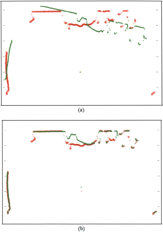
The large number of individual distance measurements that make up each of the scans from the LIDAR are analyzed by using a scan matcher, which estimates a translation and rotation to match up two consecutive scans (see Figure 2-5), using the assumption that the objects viewed have not changed or moved in the fraction of a second between scans [1]. The resulting transformation is then used as an estimate of the motion of the robot.

(a)

)M:0*

(b)

Figure 2-5: Two consecutive scans are shown in green and red. The scan matcher calculates the rotation and translation required to take the raw returns (a) and align

Chapter 3

The State Estimator

The design of the new state estimator is the central research element of this work. An accurate estimate of the current position of the robot is necessary for any type of robotic navigation. The new state estimator works by combining the data of the number of sensors on the robot over time to generate a more accurate combined esti-mate. This software module uses the extended Kalman filter, the most popular tool for robotic state estimation. Furthermore, the design presented below could be easily adapted to another system or extended to other sensors, as the core functionality is independent of the data source.

3.1

The State

The state estimator uses a 15 degree of freedom estimate of the vehicle. In three degrees of freedom each, it records (as well as 5 bias terms for the data from the

IMU) the:

" Position " Rotation " Velocity

o Acceleration

The position and orientation terms are defined in the global frame of reference, which is defined with the origin where the robot is powered on. The other terms are defined in the body frame of reference, where the origin is the center of the robot with the x-axis forward, y left and z up.

Therefore, the state vector x is defined as:

x = (x, y, z, 0, c 0, , , , , ,

,

3.2

The Data

Data is received by the state estimator asynchronously through LCM messages. Each is received at a different rate, and gives estimates of different portions of the state of the vehicle.

3.2.1

Scan Matcher Data

The scan matcher outputs an estimate of the position and yaw of the robot at 40 Hertz.

ZLIDAR (X, y, z, 0)

3.2.2

GPS Data

The GPS outputs Longitude and Latitude measurements at 1 Hertz. These are converted into the global frame using an approximation.

3.2.3

IMU Data

The IMU outputs pitch, roll and the accelerations at 100 Hertz. The IMU data is treated as though it outputs those estimates plus the associated bias

[2].

ZIMU = (<p + Bias., + BiasVp, + Bias₂, j + Biasp, z

+

Therefore: HruM =

(

0

3.3

The System Dynamics

The approximation of the system's dynamics is defined by Gt, where pt = g(pt_1) = G* * ptt_1.

0 0 0 0 0 dt*cos(0) -dt*sin(O) 0 1 0 0 0 0 dtsin(O) dtcos(0) 0 0 0 0 0 0 0 0 0 0 0 0 0 0 1 0 0 0 0 0 dt 0 0 0 0 0 0 0 0 0 0 0 0 0 0 1 0 0 0 0 0 dt 0 0 0 0 0 0 0 0 0 0 0 0 0 0 1 0 0 0 0 0 dt 0 0 0 0 0 0 0 0 0 0 0 0 0 1 0 0 0 0 dt 0 0 0 0 0 0 0 0 0 0 0 0 0 0 1 0 0 0 0 dt0 0 0 0 0 0 0 0 0 0 0 0 0 0 1 0 0 0 0 0dt 0 0 0 0 0 0 0 0 0 0 0 0 0 0 1 0 0 0 0 0dt 0 0 0 0 0 0 0 0 0 0 0 0 0 0 1 0 0 0 0 0 0 0 0 0 0 0 0 0 0 0 0 0 0 0 0 1 0 0 0 0 0 0 0 0 0 0 0 0 0 0 0 0 0 0 0 0 1 0 0 0 0 0 0 0 0 0 0 0 0 0 0 0 0 0 0 0 0 1 0 0 0 0 0 0 0 0 0 0 0 0 0 0 0 0 0 0 0 0 1 0 0 0 0 0 0 0 0 0 0 0 0 0 0 0 0 0 0 0 0 1 0 0 0 0 0 0 0 0 0 0 0 0 0 0 0 0 0 0 0 0 1 0 0 0 0 0 0 0 0 0 0 0 0 0 0 0 0 0 0 0 0 1 0 0 0 0 0 0 0 0 0 0 0 0 0 0 0 0 0 0 0 0 1 0 0 0 0 0 0 0 0 0 0 0 0 0 0 0 0 0 0 0 0 1 0 0 0 0 0 0 0 0 0 0 0 0 0 0 0 0 0 0 0 0 1

3.4

The Extended Kalman Filter

The Kalman filter, introduced in 1960, relies on the fact that observations are linear functions of a state, and that the next state is a linear function of the previous state. Unfortunately, this assumption will not hold in any but the most trivial robotic sys-tems. The extended Kalman filter (EKF) relaxes these linearity assumptions, allow-ing us to filter systems with nonlinear state transition and measurement probabilities. The extended Kalman filter utilizes the first order Taylor expansion to linearize the

measurement function h. Algorithm 3.1 states the extended Kalman filter algorithm. For a full description of the EKF, please see Probabilistic Robotics, Thrun et al., chapter 3.3 [8].

Algorithm 3.1 The extended Kalman filter algorithm [8].

Require: Previous belief state yt-, Et_1, action tt, and observation zt

1: pt = g(ut, y,_t1) 2: It = Gtlt_1GT + R 3: Kt = :tH(HEft H[+

Qt)-1

3.4.1

Noise Parameters

The testing environment used was very constrained, and thus the process noise was assumed to be small. The vehicle was stably mounted on a wheeled platform. For each specific type of environment, the process noise will have to be determined. The matrix of process noise (R) was constructed diagonally using small coefficients to keep the state estimator's covariances from reducing too much and starting to ignore data. The vector of coefficients used to make the diagonal matrix is as follows: (note: it is of length 20, corresponding to the state vector.)

Rt(diagonal)(

dt

IMU

The measurement covariance matrix

Q

to three significant figures here for readability). 4.53 x 10-5 1.28 x 10-5 4.43 x 10-4 -1.30 x 10-4 -7.22 x 10-5 1.28 x 10-5 1.09 x 10-5 1.25 x 10-4 -1.07 x 10-4 -1.37 x 10-5 4.43 x 10-4 1.25 x 10-4 4.52 x 10-3 -1.26 x 10-3 -7.20 x 10-4 -1.29 x 10-4 -1.07 x 10-4 -1.26 x 10-3 1.24 x 10-3 1.44 x 10-4 -7.21 x -1.37 x -7.20 x 10-1.44 x 10-4 3.90 x 10-4

The measurement covariance matrix

Q

horizontal _accuracyt 0.0000 0.0000 2 horizontal-accuracyt Scan Matcher

The measurement covariance matrix

Q

QLIDAR cov.x cov.xy 0 0 cov.xy cov.y 0 0

LIDAR data is constructed from the

0 0 cov.z 0 0 0 0 cov.yaw

3.5

Implementation

The EKF is implemented using the popular, open-source, Eigen matrix math library for C/C++. Data is received by subscribing to a number of LCM messages (those of the GPS, IMU, and scan matcher) in state-estimatorGPSlaserIMU.cpp, which creates and updates an object of the newly created EKF class, defined in EKF.cpp and EKF.h. Each time a message is received by the state estimator, it calls the appropriate

QIU =I

GPS

update function for the EKF. The filter is thereby updated asynchronously, at a rate equal to the combined rate of the multiple data sources, in this case: 141Hz.

Chapter 4

Results

4.1

Summary of Results

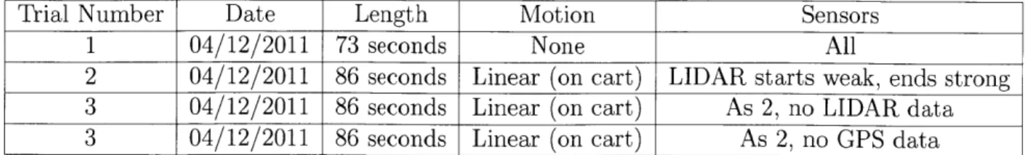
The new state estimator performed satisfactorily to complete the mission of culvert inspection. Performance was evaluated on a number of mission types (see Table 4.1). The data collection area offered clear GPS reception with a section relatively clear of obstructions and one where the LIDAR would have many strong returns (see Figure

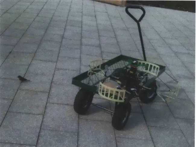
4-1). To achieve predicable motion of the platform, the quadrotor was mounted to a

cart, an rolled along a straight-line path to collect data used to test the state estimator (see Figure 4-2). With constant GPS reception, as well as good returns from the LIDAR, the state estimator was quite accurate. There was only a small degradation in performance when GPS was lost, and even without the highly-accurate LIDAR data, the scan matcher was able to use the GPS and IMU together to smooth the noisy GPS data (see Figures 4-3, 4-4, 4-5, 4-6,).

Trial Number Date Length Motion Sensors

1 04/12/2011 73 seconds None All

2 04/12/2011 86 seconds Linear (on cart) LIDAR starts weak, ends strong

3 04/12/2011 86 seconds Linear (on cart) As 2, no LIDAR data

3 04/12/2011 86 seconds Linear (on cart) As 2, no GPS data Table 4.1: Table of Test Missions

Figure 4-1: Image of the data collection area outside MIT's Stata Center. The am-phitheater in the foreground provided consistent LIDAR returns, while the relatively clear area in the background had few obstructions visible to the LIDAR. The quadro-tor UAV (on its cart) and author are shown near the bottom of the image.

Figure 4-2: Image of the quadrotor mounted on a cart for data collection.

State estimator trial 1: stationary with all sensors

meters from start in X

2 4 6

Figure 4-3: The state estimator is shown running on the data from trial 1, where the quadrotor is stationary. The inaccurate GPS data is shown by blue circles, and the state estimator's output is tightly clustered at 0,0 (its initial position) as a series of red dots.

0 Raw GPS data

x Raw scan matcher data

0 -State estimate -0 State estimate -0 ₀ 0 0 o 0 0 00 0 0 0 0 0 0 00000 0 0 I Nilc,~

State estimator trial 2: moving with all sensors

-20 -15 -10 -5 0

meters from start in X

Figure 4-4: The state estimator is shown running on the data from trial 2, where the quadrotor is pulled along a straight line path. The inaccurate GPS data is shown by blue circles, and the state estimator's output (red) is shown following, but smoothing, the output from the scan matcher (green).

State estimator trial 3: moving with only GPS and IMU data

meters from start in X

Figure 4-5: The state estimator is shown running on the data from trial 2, where the quadrotor is pulled along a straight line path, but where the LIDAR data is removed. The GPS data is shown by blue circles, and the state estimator's output is shown by red dots connected by a black line.

State estimator trial 4: moving with only LIDAR and IMU data

x Raw scan matcher data -- state estimate

state estimate

-20 -15 -10 -5 0

meters from start in X

Figure 4-6: The state estimator is shown running on the data from trial 2, where the quadrotor is pulled along a straight line path, but where the GPS data is removed (simulating a GPS-denied environment). Comparing to Figure 4-4, we can see the state estimator is quite robust against GPS failure.

Chapter 5

Conclusion

5.1

Suggestions for Future Work

The state estimator could be perfected by improving the accuracy of some of the methods used. In particular, The GPS

Q

5.2

Closing Remarks

This new state estimator enables autonomous outdoor navigation and operation of a micro-UAV. GPS is not accurate enough to control a micro-UAV alone, and can be easily corrupted further or lost altogether by any structures that introduce multi-path errors or obstruct line-of-sight to the GPS satellites. For this reason, it is essential in all outdoor autonomous robotics to fuse GPS data with other, more accurate sensors

to obtain a robust system. The capability of state estimation developed during this work could be of use for many outdoor robotics projects. By changing a handful of constants and coefficients, the filter can be adapted to use data from other sensors,

Appendix A

Source Code

./code/state-estimator-GPSlaserIMU.cpp

* state estimator GPSlaserIMU. cpp *

Created on: December 9th, 2010 Author: Nathan Serrano

* _{A new state estimator based on the Extended Kalman Filter that uses}

data from the Quadrotor 's IMU, GPS and the output of the scan matcher running on the LIDAR data.

#include <stdio .h>

#include <bot -core / bot _core . h> #include <lcm/lcm.h>

#include <Eigen/Core>

#include <lcmtypes /quadlcmtypes. h>

#include <quad _cmtypes /lcm channel names .h> #include "EKF.h"

using namespace Eigen;

static carmen3d-odometry-msg-t * smpos-msg = NULL;

static carmen3d-imu-t * imu-msg = NULL;

EKF filter ;

static bot-core-pose-t pose;

static carmen3d-quad-gps-data-msg-t * gps-msg = NULL; static const bool DEBUGOUTPUT = FALSE;

static void gps-advanced-handler(const lcm-recv-buf-t *rbuf

__attribute-_ ((unused)), const char * channel -attribute-_ ((unused) const carmen3d-quad-gps-data-msg-t * msg,

void * user -attribute_ ((unused)))

{

if (gps-msg != NULL){

carmen3d-quad-gps-data-msg-t-destroy(gps-msg);

}

gps-msg = carmen3d _quad-gps-data-msg-t _copy (msg);

//send to the filter , get a updated pose

int sucess = filter . filterGPS (*gps-msg , &pose)

//publish pose if (sucess != 0)

{

bot _corepose t-publish (lcm, "POSEGPSLASERIMUCHANNEL"

&pose); i f (DEBUG-OUTPUT)

fprint f ( stderr ," Published-from _GPSdata.\n")

}

}

static void sm pos-handler(const lcm-recv-buf-t *rbuf __attribute_ ((

unused)) , const char * channel __attribute_- ((unused)), const

carmen3d-odometry-msg-t * msg,

void * user -_attribute__ ((unused)))

{

if (sm-pos-msg != NULL){

}

sm-pos-msg = carmen3d-odometry-msg-t-copy(msg);

/send to the filter , get a updated pose

int sucess = filt er . filterLIDAR (*sm-pos-msg , &pose)

//publish pose

if (sucess != 0)7/If it worked

{

bot core-poseA publish (1cm, "POSEGPSLASERIMUCHANNEL",

&pose); i f (DEBUG-OUTPUT)

fprintf ( stderr ," Published-from-LIDAR-data.\n")

}

}

static void imu-handler(const lcm-recv-buf-t *rbuf __attribute_ ((unused

)), const char * channel __attribute- ((unused)), const

carmen3d-imu-t * msg, void * user __attribute ((unused)))

{

//fprintf(stderr,"imuhandler called.\n");

if (imu-msg != NULL){

carmen3d-imu-t-destroy (imu msg);

}

imu-msg - carmen3d-imut -copy(msg);

/send to the filter , get a updated pose

int sucess = filter filterIMU (*imu-msg, &pose);

/publish pose

if (sucess != 0)

{

bot _corepose t _publish (lcm, "POSEGPSLASERIMUCHANNEL",

&pose) ; i f (DEBUGOUTPUT)

fprintf ( stderr ," Published -from-IMU-data.\n")

}

}

int main(){

fprintf (stderr , "Startin g-GPS/LIDAR/IMU-state-estimator .\n");

lcm = bot lcm-get global (NULL);

carmen3dquadgps-data-msg-tLsubscribe (1cm,

ASCTECGPSADVANCEDCHANNEL, &gps _advanced _handler , NULL);

//longitude and latitude

//Scan matcher channels.

carmen3d-odometry msg-t-subscribe (1cm, SCAN-MATCHPOS-CHANNEL,

sm-pos-handler , NULL); //world coordinates - this is

integrated and relative to the start location where the quad was turned on.

//carmen3d odome trymsg t subscribe (1cm, SCANATCHRELCHANNEL, sm-rel-handler , NULL); /body coordinate relative motion

-I should probably use this and differentiate it myself, but might not matter.

// imu-t contains rotation rates and liner accelerations

carmen3d-imu-t -subscribe (1cm, IMUCHANNEL, &imu-handler, NULL);

fprintf ( stderr ,"Subscriptions -done, -ready-to -run.\n);

// run while (1){ lcm-handle(lcm);

}

}

*

* Created on: Jan 24, 2011

* Author: Nathan E. Serrano

#ifndef EKF_H_ #define EKF_H_

#include <Eigen/Core>

#include <bot core/bot core .h> #include <lcm/lcm.h>

#include <lcmtypes/quad lcmtypes. h>

#include <fstream> using namespace std;

using namespace Eigen;

class EKF { public:

EKF();

virtual ~EKF();

int filterIMU(const carmen3d-imu-t& imu-msg, bot-core-pose-t *pose);

int filterGPS(const carmen3d quad gps _data-msg-t& gps-msg, bot-core-pose-t *pose);

int filterLIDAR(const carmen3d-odometry-msg-t& sm-pos-msg, bot-core-pose-t *pose)

private:

int FilterUpdate (long utime)

MatrixXd g(VectorXd mutminus1, MatrixXd Gt); MatrixXd updateG ( VectorXd mutminus1);

MatrixXd h(VectorXd mutbar, MatrixXd Ht);

MatrixXd Qgps(int num-sats, double horizontal-accuracy); bot-core-pose-t get pose(VectorXd mut, MatrixXd sigmat); MatrixXd Qlidart (carmen3d-point-cov-t cov);

MatrixXd Qgps-t(int num-sats, double horizontal-accuracy); void update-filter-with-data(VectorXd zt);

long current-utime ; VectorXd mutminus1; VectorXd mut; VectorXd mutbar; MatrixXd sigmaO; MatrixXd sigmatminus1; MatrixXd sigmat; MatrixXd sigmatbar; MatrixXd Gt; MatrixXd Qt; MatrixXd Ht;

MatrixXd Rconst ant; MatrixXd Q_IMU; MatrixXd Q_LIDAR; MatrixXd Q-GPS; MatrixXd Kt; MatrixXd HIMIU; MatrixXd HGPS; MatrixXd HLIDAR; BotGPSLinearize gps-linearize bool linearize initialized double dt; ofstream mubarfile; ofstream sigmabarfile ofstream Gtfile ; ofstream ztgpsfile ofstream ztimufile ofstream ztlidarfile ofstream Ktfile ; ofstream mutfile ofstream sigmatfile

};

./code/EKF.cpp

* EKF.cpp *

* Created on: Jan 24, 2011

* Author: Nathan E. Serrano

*7

#include <bot _core / bot _core .h>

#include <bot _core/gps-linearize .h> #include <lcm/lcm.h>

#include <lcmtypes/quad lcmtypes.h>

#include <quad _lcmtypes /lcm channel-names .h>

//#include <quadEKF/quadEKF _utils .hpp>

#include "EKF.h" #include <Eigen/Core> #include <Eigen/LU> #include <iostream> #include <fstream> using namespace std;

static const int STATELENGTH = 20;//The number of state variables static const double INITALSIGMA = 100.0;

static const int NUMLIDARVARS = 4; static const int NUMIMUVARSEKF = 5; static const int NUM GPSVARS = 2;

static const VectorXd mu0 = VectorXd:: Zero(STATELENGTH); /the initial state

static const double LCM-UTIMETOSECONDS = 1.0/1000000.0; // LCM's utime is a long int , corrasponding to microseconds (millionths of a

second) since the unix epoch.

static const bool OUTPUTJNTERNALDATATOFILES = TRUE;

using namespace Eigen;

mutminus1 (STATFTENGTH), mut (STATELENGTH) ,

mut bar (STATELENGTH),

s ig m aO0 (STATELENGTH, STAIIELENGTH), sigmatminus (STATELENGTH,STATELENGTH) s ig m at (STATELENGTH, STATELENGTH) , s ig m at b ar (STATELENGTH,STATELENGTH) ,

Gt (STATELENGTH, STATELENGTH) , //s t a t e t r a n s it i o n

model

R _ c ons t ant (STATELENGTH,STATFIENGTH),

QJMU (NUMIMUVARSEKF, NUMJMUVARSEKF),

QIDAR (NUMLIDARVARS, NUMLIDARVARS),

QGPS (NUMGPSVARS, NUMGPSVARS) ,

Kt (STATELENGTH,STATE[ENGTH) , //Kalman Gain

HIMU (NUMIMUVARSEKF, STATEIENGTH), HGPS (NUM-GPS-VARS,STATELENGTH) , HLIDAR(NUMLIDARVARS,STATELENGTH)

7/

/state vector is X = (x,y,z, theta ,phi,psi ,x ',y ',z ',theta ',phi',

psi ',x '', y '', z '', biasx , biasy , biasz , biastheta , biaspsi)

/theta , phi , psi are the Euler angles

/7 x,y,z,theta,phipsi are represented in the global frame, with origin at where the vehicle is initialized.

//values chosen arbitrarily to be of proper order of magnitude double angleSigma = 100.0;

double angledotsigma = 1.0; double xdoubledotsigma = 100.0;

VectorXd sigmacoeff (STATELENGTH);

sigmacoeff << 100.0, 100.0, 100.0, angleSigma, angleSigma, angleSigma, 1.0, 1.0, 1.0, angledotsigma , angledotsigma,

angledotsigma , xdoubledotsigma , xdoubledotsigma , xdoubledotsigma , xdoubledotsigma , xdoubledotsigma,

xdoubledotsigma , angleSigma , angleSigma;

mutminus1 = mut = mu0;

mu0;

sigmatminus1 = sigma0; sigmat = sigma0;

//covariance matrix of unobservable measurement noise //values determined empirically from covariance matrix of

stationary data collection

//massive numbers of sigfigs because this is copy/pasted from matlab QIMU << 4.53494423651763*pow(10, -05) 1.28573585495108*pow(10,-05), 0.000443408744921134, -0.000129645506516096, - 7.21757489664307*pow(10, -05) 1.2 8573585495108*pow(10,-05), 1.09 3 0 0 6 01750000*pow(10,-05) 0.000124641513337291, -0.000106661424279292, -1.36696431544322* pow(10, _{-05) ,} 0.000443408744921134, 0.000124641513337291, 0.00452196485212367, -0.00126237612649800, -0.000720439848362413, -0.000129645506516096, -0.000106661424279292, -0.00126237612649800, 0.00123768655591818, 0.000144258575568637, - 7.21757489664307*pow(10,-05) -1.36696431544322*pow (10, -05) -0.000720439848362413, 0.000144258575568637, 0.000389509155434245;

QLIDAR << MatrixXd:: Identity (NUMLIDARVARS,NUMLIDARVARS);

QGPS << MatrixXd:: Identity (NUMGPSVARS,NUMGPSVARS);

HIMU << 0,0,0, 0,1,0, 0,0,0, 0,0,0, 0,0,0,

pitch estimate from IMU

0,0,0, 0,0,1, 0,0,0, 0,0,0,

roll estimate from IMU

0,0,0, 0,0,0, 0,0,0, 0,0,0,

xdd estimate from IMU

0,0,0, 0,0,0, 0,0,0, 0,0,0,

ydd estimate from IMU

0,0,0, 0,0,0, 0,0,0, 0,0,0,

zdd estimate from IMU

0,0,0,1,0, / 0,0,0, 0,0,0,0,1, /7 1,0,0, 1,0,0,0,0, / 0,1,0, 0,1,0,00,7/ 0,0,1, 0,0,1,0,0; HGPS << 1,0,0, 0,0,0, 0,0,0, 0,0,0, 0,0,0, 0,0,0,0,0, x 0,1,0, 0,0,0, 0,0,0, 0,0,0, 0,0,0, 0,0,0,0,0; y HLIDAR << 1,0,0, 0,0,0, 0,0,0, 0,0,0, 0,0,0, 0,0,0,0,0, x 0,1,0, 0,0,0, 0,0,0, 0,0,0, 0,0,0, 0,0,0,0,0, y 0,0,1, 0,0,0, 0,0,0, 0,0,0, 0,0,0, 0,0,0,0,0, z 0,0,0, 1,0,0, 0,0,0, 0,0,0, 0,0,0, 0,0,0,0,0; yaw from quad. cfg noise

VectorXd R-params(STATELENGTH);

//1cm process noise

R-params << pow (1.0, -5.0) , pow (1.0, 5.0) ,0, 0,0 ,0, 0 ,0 ,0, 0,0,0, 0,0,0, 0,0,0,0,0;

R-constant. diagonal () = R-params;

current-utime = -1; /long declared in .h file

//bot-timestamp-now (); would get current time. Does not seem to work with logs

linearize-initialized = false; mubarfile .open(" mut _bar . txt");

sigmabarfile .open(" sigma-bar . txt");

Gtfile.open("Gt.txt"); ztgpsfile .open("ztGPS .txt"); ztlidarfile .open("ztLIDAR. txt") ztimufile .open("ztIMU. txt" Ktfile .open("Kt.txt"); mutfile.open("mut. txt"

sigmatfile .open(" sigma-t . txt");

}

int EKF:: FilterUpdate (long new-utime)

{

if (current-utime = -1) // has not been initialized

{

current-utime new-utime;

fprintf (stderr ," _{filter -utime- initialized -to-%li -.\n"}

new utime)

}

dt = new-utime - current-utime;

if(new-utime < current-utime)

{

//printf("ERROR: Data received from utime: %li which is

> the current internal filter utime: %li.\n", new-utime , current-utime);

fprintf (stderr , "ERROR:-old-data-received . -dt-=-%f ,dt_ set -to -. 01 -seconds _\n" , dt ) ;

dt = 10000; /corasponds to the time delay between 100Hz updates //return -1;

}

}

}

MatrixXd EKF:: g(VectorXd mutminus1, MatrixXd Gt)

{

return Gt * mutminus1;

}

MatrixXd EKF:: updateG (VectorXd mutminus1)

{

//fprintf(stderr , "dt is

double yaw = mutminusl(3)

double c = cos(yaw); double s = sin(yaw); double xd = mutminus1 (6) double yd = mutminus1 (7) double dx-dxd = dt double dx-dyd -dt double dx-dt = dt * double dy-dxd = dt double dy-dyd dt double dy-dt - dt * MatrixXd

//

Gupdate (STATELENGTH, STATTEFNGTH);

x, y, z, angles _{x ',y ',z} ',

x Bias x,y,z,pitch ,roll

< 1 ,0 ,0, 0 ,0 ,0 , dx-dxd , dx-dyd ,0 , 0,0,0, 0,0,0,0,0, //x (global) 0,1,0, 0,0,0, dy-dxd,dy-dyd,0, 0,0,0, 0,0,0, 0,0,0,0,0, 0,0,1, 0,0,0, 0,0,0, 0,0,0, 0,0,0, 1,0 dt ,0 ,0 yaw 0,0,0, 0,1 0,dt ,0, pitch 0,0,0, 0,0 0,0,dt roll ,0, 0,0,0, 0,0,0, 0,0,0, 0 ,0,dt, 0,0,0,0,0, 0,0,0, 0,0 ,0 ,0 ,0, 0,0,0, 0,0 ,0 ,0 ,0, 0,0,0, 0,0,0,0,0,

0,0,0, 0,0,0, 0,0,0, dt,0,0, //xdot (body) 0,0,0, 0,0,0, 0,0,0, 0,dt,0,

/ydot

x bias of IMU (body)

0,0,0, 0,0,0, 0,0,0, 0,0,0,

0,0,0,

y bias of IMU 0,0,0, 0,0,0, 0 0,0,0, 0,0,0, z bias of IMU 0,0,0, 0,0,0, 0 0,0,0, 0,0,0,

pitch bias of IMU

0,0,0, 0,0,0, 0 0,0,0, 0,0,0,

roll bias of IMU

,0,0, 0,0,1,0,0, ,0 ,0, 0,0,0,1 ,0, ,0 ,0, 0,0,0,0,1; i f (OUTPUTINTERNALDATA-TOFILES) {

Gtfile << Gupdate << endl << endl;

}

return Gupdate;

MatrixXd EKF::h(VectorXd mutbar, MatrixXd Ht){

return Ht * mutbar;

}

int EKF:: filterIMU(const carmen3d-imu-t& imumsg, bot-core-pose-t * pose)

{

long new-utime = imu-msg. utime;

if(FilterUpdate(new-utime) = -1) /this calls the filter update equations

{

return 0;

dt = new-utime current-utime;

/get the roll , pitch , yaw from the IMU's quaternians

double imurpy [3];

bot-quat-to-roll-pitch-yaw(imu-msg.q, imu-rpy); double accel [3];

double rpy[3] = { imu-rpy[0] , imu-rpy[1] , 0.0 };//ignore yaw since we want acceleration in "body 2D" frame

bot _roll pitch-yaw-to quat (rpy , orientation) ;

//get-accel-from-imu (orientation , imu-msg. linear-accel , accel);

double imu-accel [3] = {imu-msg. linear accel [0] ,imumsg. linear-accel [1] ,imu-msg. linear-accel [2] };

//rotate IMU to vertical and remove gravity

bot-quat-rotate-to (orientation , imu-accel , accel);

double gVec [3] = { 0, 0, -9.81 };

bot-vector subtract 3d ( accel , gVec, accel)

/vehicle acceleration is opposite of IMU

accel [0] = -accel [0] accel [1] = -accel [1]; accel [2] = -accel [2];

//put message data in vector z_t

VectorXd zt (NUMIMUVARSEKF);

7/

zt << imu-rpy [1] , imu-rpy [0] , accel [0] , accel [1] , accel [2];

if (OUTPUTJNTERNALDATATOFILES) {

ztimufile << zt .transpose () << endl << endl;

}

//Q is fixed for the IMU

//measurement noise covarience matrix

Qt = QJMU;

Ht = TMU; /size is NUMIMUVARSEKFxSTATELENGTH

update filter with-data (zt); current-utime = new-utime;

//Algorithm step 6

*pose _{= get pose (mut, sigmat)}

}

int EKF:: filterGPS (const carmen3dquad_gpsdata-msgt& gps-msg, bot-core-pose-t *pose)

{

{

.longitude; /was logitude[sic]

.latitude ,lon };

long new utime = gps msg. utime;

if( FilterUpdate(new-utime) = -1)

{

return 0;

//fprintf(stderr ,"mu-t bar: X: mutbar(1));

dt = new utime - currentutime

//fprintf(stderr,"dt: %f \n",

if (! linearize-initialized )

%f Y: %f \n", mutbar(O),

dt);

bot-gps-linearizeinit (&gps-linearize , 11); //

libbot2 externals file gps-li'nearize. c

linearize-initialized = true;

fprintf (stderr ," Linearize initialized _\n");

}

//fprintf (stderr ,"lon: %f and lat : %f \n", 11 [0], il [1]); double xy [2];

bot gps linearize to-xy(&gps-linearize , 11 , xy);

//fprintf(stderr,"zt: X: %f and Y: %f \n",xy[O],xy[l]);

//put message data in vector z_t

VectorXd zt (NUMGPSVARS) ; //data double double double Ion lat 11

zt << xy(0], xy [1];

i f (OUTPUTINTERNALDATATOFILES) {

ztgpsfile << zt . transpose () << endl << endl;

I

//use this data to update/create Q

Qt = Qgps-t (gps-msg. numSatellites , gps-msg. horizontal accuracy) Ht = HGPS; update-filter-with-data (zt) current-utime = new-utime; //Algorithm step 6

*pose = get-pose (mut, sigmat)

return 1;

}

else

return 0;

}

MatrixXd EKF:: Qgps-t(int num-sats , double horizontal-accuracy)

{

MatrixXd Qgps(NUMGPSVARS,NUMGPSVARS);

Qgps << pow(horizontal-accuracy ,2.0) , 0.0, 0.0 , pow( horizontal-accuracy ,2.0) ;

//fprintf(stderr ,"Qgps diagonal: %f \n",pow(horizontal accuracy ,2.0));

return Qgps;

int EKF:: filterLIDAR (const carmen3d-odometry-msg-t& sm-pos-msg , bot-core-pose-t *pose)

//data in world/global coordinates

/get the roll , pitch , yaw from the quaternians

// LIDAR only measures yaw

double lidar-rpy [3];

bot-quat-to-roll-pitch-yaw (sm posimsg. rot-quat , lidar-rpy);

double xyz [3]= {smipos-msg. trans vec [0] , sm-pos-msg. trans vec

[1] , sm pos-msg. trans vec [2] };

long new utime smpos-msg. utime;

if(FilterUpdate(new-utime) -- -1) //if the call to update the filter fails

{

return 0;

dt = new-utime current-utime ;

//put message data in vector z-t

Ve ctor X d z t (NUMLIDARVARS) ;

// ), y , z ,

zt << xyz[0] ,xyz[1] ,xyz[2] , lidar-rpy [2];

i f (OUTPUTINTERNALDATATOFILES) {

ztlidarfile << zt.transpose() << endl << endl; } Qt = Qlidar t(smpos-msg.cov); Ht = HLIDAR; update-filter-with-data(zt) current-utime = new-utime; //Algorithm step 6

*pose = get-pose (mut, sigmat)

return 1;//sucess!

}

MatrixXd EKF:: Qlidart (carmen3dpointcov-t cov)

{

//updates the EKF with the data in zt as well as the new values of Ht,Kt ,Qt,ect. (which are class variables updated in the filter fuctions).

void EKF:: update-filterwith-data (VectorXd zt)

{

//Algorithm step 3

Kt = sigmatbar * Ht. transpose () * ((Ht * sigmatbar. transpose () * Ht. transpose () + Qt) . inverse () );

i f (OUTPUTINTERNALDATATOFILES) {

Ktfile << Kt << endl << endl;

}

//Algorithm step 4

mut = mutbar + Kt*(zt - h(mutbar,Ht)); i f (OUTPUTINTERNALDATATOFILES) {

mutfile << mut. transpose() << endl << endl;

}

//Algorithm step 5

sigmat = (MatrixXd:: Identity (STATELENGTH,STATELENGTH)

* sigmatbar;

Kt * Ht) 0,

i f (OUTPUTINTERNALDATATOFILES) {

sigmatfile << sigmat << endl << endl;

}

}

bot-core-pose-t EKF::get-pose(VectorXd mut, MatrixXd sigmat)

{

bot-core-pose-t pose; pose utime = current utime pose.orientation [3] = 0;

for (int i = 0; i<3;i++)

{

pose. pos[i] mt(i); pose. vel[ i] mut( i +6);

pose. orientation[ i] = mut(i+3); pose. rotation-rate [i] = mut(i+9);

pose. accel[i] = mut( i+12);

}

//fprintf(stderr,"%f, %f, %f,%f \n", pose. pos fO, pose. pos [1], pose .vel[0],pose. vel[1]);

return pose;

}

EKF::EKF() {

Bibliography

[1] Abraham Bachrach, Ruijie He, and Nicholas Roy. Autonomous flight in unknown

indoor environments. International Journal of Micro Air Vehicles, 2010.

[2]

[3]

helicopter. In Digital Avionics Systems Conference, 2002. Proceedings. The 21st, volume 2, pages 8C1-1 - 8C1-19 vol.2, 2002.

[4] R E Kalman. A new approach to linear filtering and prediction problems 1.

Journal Of Basic Engineering, 82(Series D):35-45, 1960.

[5] D. Mellinger, N. Michael, and V. Kumar. Trajectory generation and control for

precise aggressive maneuvers with quadrotors. In Proceedings of the International

Symposium on Experimental Robotics, Dec 2010.

[6] Seung-Min Oh. Multisensor fusion for autonomous uav navigation based on the

unscented kalman filter with sequential measurement updates. In Multisensor

Fusion and Integration for Intelligent Systems (MFI), 2010 IEEE Conference on,

pages 217 -222, sept. 2010.

[7] MIT DARPA Grand Challenge Team. lcm: Lightweight communications and

marshalling. http://code.google.com/p/lcm/, 2007.

[8] Sebastian Thrun, Wolfram Burgard, and Dieter Fox. Probabilistic Robotics. The

MIT Press, September 2005.