Birdcage resonator design in magnetic resonance imaging

BIRDCAGE RESONATOR DESIGN

IN MAGNETIC RESONANCE IMAGING

by

PETER SPRENGER

Interkantonales Technikum Rapperswil, Switzerland, 1989

Submitted to the Department of Nuclear Engineering and the Department of Electrical Engineering and Computer Science

in Partial Fulfillment of the requirements for the Degrees of Master of Science in Electrical Engineering and Computer Science

and

Master of Science in Nuclear Engineering Massachusetts Institute of Technology

June 1995

¢ Peter Sprenger, 1995. All rights reserved

The author hereby grants to MIT permission to reproduce and to distribute publicly copies of this thesis document in whole or in part

Signature

of

Author

...

....

...

...

Certified

by

...

,,,., . , ...

...

.... ...

J Jerome L. Ackerman, Massachusetts Genearal Hospital 9parntm nt of ~lectri al Engineering and Computer Science Thesis Advisor

Certified

by.. ...

Ribert M. Weisskoff, Massaeiusetts General Hospital Massachusetts General Hospital, Imaging Center Thesis Advisor

Certified

by....

David G. Cory, Professor at the De u of Nuclear Engineering Thesis Reader

Accepted

by

... ...

...

AllaF. HemI*Ti~rmaa NID Committe on Graduate Students

Accepted by .. y, , ... · · · · .

F.R. Morgeithaler,'air, EECS Committee on Graduate Students

Barker Eng

BIRDCAGE RESONATOR DESIGN

IN MAGNETIC RESONANCE IMAGING

by

PETER SPRENGER

Submitted to the Department of Nuclear Engineering and the Department of Electrical Engineering and Computer Science

in Partial Fulfillment of the requirements for the Degrees of Master of Science in Electrical Engineering and Computer Science and

Master of Science in Nuclear Engineering

ABSTRACT

Circuit equations for the general Birdcage resonator are solved with a polyno-mial approach and an expression for the resonant frequencies is derived. The results are compared with numerical calculations and with experiments on a 12 mesh, low pass Birdcage. A design procedure for low pass Birdcages, which follows directly from the polynomial analysis, is presented. It is shown that the resonant frequencies can be divided into low and high impedance res-onant modes and that the total number of resres-onant frequencies is equal to the number of meshes. The angular current distribution in the legs of the resonator is derived using the polynomial approach. Two methods of measuring the cur-rents in the legs of the resonator are proposed and verified experimentally. A resonator tuned to its second mode can be viewed as a surface coil wrapped around the sample and thus yields an increased Signal to Noise ratio at the edge of the resonator. This increase is calculated theoretically for a spherical sample and the experimental value is in good agreement.

A description of the transmission line is included since the concept is useful for the understanding of the Birdcage resonator.

Thesis Supervisor for NED: Dr. Robert M. Weisskoff Thesis Supervisor for EE: Dr. Jerome L. Ackerman

Table of contents

3.

Birdcage resonator

3.2 Principle of the Birdcage Resonator 35

3.3 Resonance frequencies 38 3.4 Current distribution 52 3.5 Numerical Methods 58 3.6 RF Field distributon 67 3.7 SNR considerations 72 3.8 Experimential results 76

4.

Practical consideration

7.

Final remarks / Acknowledgements

103

Appendix

1.

Introduction

1.1

Thesis description

Magnetic resonance imaging (MRI) is one of various mapping modalities that have been applied for the creation of images. The most important applica-tion is its use as a medical diagnostic tool. One of the main advantages of MRI over conventional CT (X-ray) tomography are the relatively low photon ener-gies, in the order of 10- 7eV, compared to 10-1000keV used in CT's [1]. This advantage however results in a much weaker received signal. Several experi-mental techniques can be applied to enhance the sensitivity of an MR image. In particular, if the object does not change in time, the MR experiment can be repeated and the collected information averaged yields an enhanced signal to noise ratio. In medical diagnostics however imaging time is limited and patients cannot be assumed to be rigid objects.

A particular important piece of the MRI scanner hardware is the sensor which picks up the electro magnetic radiation, produced by the magnetic moments of the nuclei inside the object. Several types of different sensors (in fact these are wire loops called coils) are used in MRI, depending on the object to be imaged and the type of experiment used. A particular design of such a coil is subject of this thesis. It provides an increased sensitivity over a limited spatial section. Since this sensor is intended to be used for functional MRI, the region of interest is the cortex of the human brain. Surface coils have previously been used to pick up the signal at a specific spatial point. The approach used here, is a special design of a Birdcage resonator [2], tuned to a resonance mode which covers a spatial area close to the one of the human cor-tex.

The thesis introduces the basic concepts of coil design in NMR (chapter 2) and presents a new way of predicting the resonance frequencies of Birdcage resonators and compares the results with existing theories [2,3] (chapter 3.3 .. 3.5) The improved sensitivity of a Birdcage tuned to the second mode (gradi-ent Birdcage) is shown (chapter 3.7). Theoretical predictions are compared with experiments. (chapter 3.8) A useful tool to adjust Birdcage resonators is presented in chapter 4.

1.2

The MR experiment

In order to understand the objective of this thesis, it is useful to first sum-marize the NMR experiment [4,5].

Consider a system at the microscopic level characterized by the quantum mechanical angular momentum L = j, wherej is the angular momentum quantum number, and h is Planck's constant. The absolute value squared of the angular momentum is given by

EQ1

L2 = [j (j+ 1) ] 2.

A particle with angular momentum has a magnetic dipole moment whose magnitude is given by

EQ2

= yhfj)(j

+)

where y is the magnetogyric ratio. The energy of the magnetic moment g in the presence of a static magnetic field H is,

EQ3

E = - . H = -Hcos0 ,

where 0 is the angle between the magnetic moment and the magnetic field. Classically, a magnetic moment can assume any orientation with respect to the magnetic field i.e. 0 can have any value from 0 to nr. However, quantum mechanics restricts the number of such orientations such that the projection of

It upon the magnetic field direction is limited to a finite set of values. Its

pro-jection upon the magnetic field is ymf, where m is restricted to the follow-ing,

EQ4

m = j, (j - 1), (j- 2), ...

(j-2), -(j- 1), -j

-The proton has an intrinsic angular momentum (spin) of S=1/2. -The magnetic moment associated with spin is given by,

EQ5

IlI = yh-lS(S+l) .

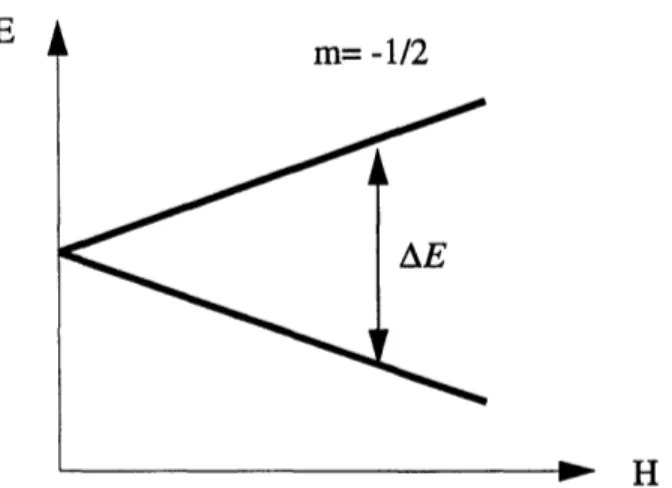
For the proton, y is 265.5x106 rad s-T l. Thus a proton in a magnetic field has only two allowed states (i.e. +/- 1/2). The energy separation between these states are given by,

EQ6

AE = yhH .

E

m= -1/2

AE

14

Fig. 1: energy difference as a function of magnetic field

Classically, the change of angular momentum over time (i.e. dL/dt ) is equal to the applied torque t = x . Hence, a magnetic dipole moment in a magnetic field will experience a time rate of change of angular momentum. From EQ1 and EQ2 we know that

EQ7

= yL, and thus we can write:

EQ8

d

= Y(aX

t.

Since the torque acting on a system is perpendicular to both !t and 1, the resulting motion will be a precession of ft about the magnetic field. Let z be the direction of the magnetic field and Mx, My and Mz be the components of

t . Now suppose a radiation field of frequency o = yHo is impressed upon a system of protons having an x-component whose time dependence

0

isHx = Hxcos (cot) . Such a linearly polarized field may be expressed as the

a field that rotates about the z-axis in a counter clockwise manner, while H1

rotates about the z-axis clockwise. The only component of Hxthat affects the

magnetization vector is H, which rotates in the same sense as does the preces-sion of the magnetization vector. In the rotating frame, Hr remains in phase with M imparting a constant torque upon the latter. This torque causes M to undergo a continuous increase in its polar angle 0 . The increase in0 will con-tinue as long as the system is exposed to the oscillating field H. The angular motion of M is called nutation. Clearly the nutation frequency depends lin-early on the strength of the of the oscillating field H.

Suppose the oscillating field H is applied for a period of it/20 0 then the

magnetization M will be aligned parallel to the y axis. This is not a state of thermal equilibrium; hence the system will move towards thermal equilibrium. During this time the oscillating magnetization will induce an EMF in the antenna which previously generated the oscillating field H.

A special antenna (called Birdcage resonator) which creates the field H and receives the magnetization M is subject of this thesis. An improved antenna design will affect both, the nutation frequency and the intensity of the induced EMF [6].

2.

Coil design

2.1

Introduction

The purpose of an NMR coil is to create a magnetic RF field to perturb the spin system. Therefore the design is focused on the optimization of the

mag-netic field produced by the coil. The photon energy is proportional to the static magnetic field Bo and is in the order of 0.5eV which corresponds to a fre-quency of approx. 100MHz (see 1.2). This frefre-quency range is heavily used by broadcasting stations, telecommunications etc. and thus a well investigated field of engineering is available to the coil designer. In fact we will use basic knowledge in radio engineering i.e. impedance matching, resonance networks, transmission lines etc. to develop a new coil design. An ideal NMR coil has the following characteristic:

a) magnetic field intensity and phase is the same at any point in space b) no heating of the coil (i.e. no resistive losses)

c) no power break down

d) no electrical field within the subject

In practice none of these ideal characteristics can be met. The optimization of a particular characteristic has to be compromised by a decreased performance of another aspect. For this reason many different coil designs are used. In this work we concentrate on the optimization of the sensitivity in a particular region of interest. First however we want to introduce a few basics in the world of coil design.

2.2

Transmission Lines

Transmission lines in the coil design for NMR have a two fold significance. First they deliver the electromagnetic energy from the radiation source (i.e. the

RF amplifier) to the coil and the small signal received by the coil (i.e. the NMR signal) to the RF receiver. To have an optimum energy transfer, the

devices (coils, receivers transmitters etc.) inter connected with transmission lines have to be matched. In chapter 2.3 we will explore the concept of match-ing. Second, transmission lines can be used as models to gain a better under-standing of special NMR coils (i.e. Birdcage resonators). Here the concept of transmission lines is introduced as it is applicable to the design of NMR coils.

2.2.1 Overview

According to the electromagnetic model [11], time varying charges and currents are sources of electromagnetic fields and waves. The waves carry electromagnetic power and propagate in the surrounding media with the velocity of light (in vacuum). In open space power transmission is very ineffi-cient. Even when a source radiates with the aid of highly directive antennas, its power spreads over wide range and thus resulting in a low power density. For an efficient point to point transmission of power, the source energy must be guided. Here we consider the transmission of transverse electromagnetic waves (TEM) in coaxial transmission lines, since this is most commonly used in NMR.

The general transmission-line equation can be derived from a circuit model in terms of resistance, inductance, conductance and capacitance per unit length of the line. From these equations, all the characteristics of wave propagation along a given line can be derived and studied. The investigation of time-har-monic steady state properties of transmission lines are facilitated by the use of graphical charts, which eases the necessity of repeated calculations with com-plex numbers. The best known and most widely used graphical chart is the Smith Chart.

2.2.2 General transmission line equations

conductors. The distance of separation between them is small in comparison with the operating wavelength. Since ordinary electric networks have physical dimensions much smaller than the operating wavelength, they can be repre-sented by lumped parameters. The voltage between the conductors and the currents along the line are closely related to the transverse components of the electric and magnetic field. We find that the dependence of these field compo-nents on the transverse coordinates is the same as under static conditions. Thus the parameters of a transmission line can be determined by methods used under static conditions. Transmission lines differ from ordinary electric cir-cuits in one important feature. The physical dimensions of electric networks are very much smaller than operating wavelength whereas transmission lines are usually longer than the operating wavelength and may even be several wavelengths long. In lumped element circuits it is assumed that there are no reflection and standing waves. Therefore a lumped parameter model of the transmission line can only be valid if the line is much shorter than the operat-ing wavelength. This leads to the concept of distributed circuits parameters throughout the entire length of the transmission line and lumped element parameters are given for a differential length dz. Consider a transmission line with length dz and the following parameters:

-R, resistance per unit length [ f/m] -L, inductance per unit length [Vs/Am]

-G, conductance per unit length [-1 /m] -C, capacitance per unit length [As/Vm]

Then we can draw the equivalent lumped electric circuit for the length dz: The quantities v(z,t) and v(z+dz,t) denote the instant voltages at position z and z+dz and i(z,t), i(z+dz,t) the currents at z and z+dz along the transmission line. We can apply Kirchoff's voltage law,

R dz _i(z+dz,t)

i(z,t)

G dz v(z+dz,t)

Fig.2: Transmission line equivalent circuit EQ9

v (z + dz, t) - v (z, t) = Ri(, t) dz

Similarly we apply Kirchoffs current law, EQ10 i (z + dz, t) - i (z, t) = Gv(z+dz,t) + dz

+ L4i(z,t)

at

C-v (z

As dz approaches zero EQ 9 and EQ 10 reduce to, EQ11

a

+

ai

(z, t)

at

at

EQ11 and EQ12 are the general transmission line equations. Since here we are primarily interested in harmonic time dependence, we can rewrite EQ11 and EQ12,

v(z,t)

EQ13

-V(z)

= (R +joL)I(z)

a-I(z)

= (G+jo(C)V(z)

where 0) is the frequency of the sinusoidal signal. EQ13 and EQ14 are linear and thus no harmonics can occur. Note that the current and the voltage are function of the spatial coordinate (i.e. z) only. Extracting V(z) from EQ 14 and substituting into EQ13 and similarly solving for I(z) in EQ13 and substituting into EQ14 yields the time harmonic transmission line equations,

EQ15 2 V(z) = 2V(z) dz2 EQ16 d2 dz2(z) = 21 (z)

where is a complex number called the propagation constant: EQ17

y

= /(R+joL) (G+joC) = a+j

.

We can clearly see that the transmission line is completely defined by its dis-tributed parameters R,L,G,C. In general, these quantities depend on 0 in a complicated way. However we will assume that these transmission line param-eters depend only on the physical dimensions of the transmission line.

2.2.3 Coaxial transmission line parameters

As we have seen, the knowledge of R,L,G,C allows us to completely char-acterize the transmission line. A coaxial cable consists of an inner conductor and an outer conducting shield separated by a dielectric medium. This struc-ture has the important advantage of confining the electric and magnetic fields entirely within the dielectric region and little external interference is coupled into the line. Most NMR instruments use coaxial cable as wave guides since they are very easy to handle and the cable losses (represented by R and G) are reasonably small. A cross section of the line is shown in the figure below.

rwt. · qP- Fvln .1 ,r

(hieLld)

inner aonc

di leao tr

taterial

Fig.3: Cross section of a coaxial transmission line The transmission line parameters are,

EQ18

R = 21(1+

[/m]

EQ21

G

=

IS/m]

log (a/b)

where a is the conductivity, the permeability, the dielectric constant of the material between the inner conductor and the shield. gc and c represent the permeability and the conductivity of the conductor material. Note that in EQ18 the square root term is the real part of the intrinsic impedance which is related to the skin effect. For our purposes we can set R=O since the conductiv-ity of the conductors in a transmission line is high and the frequency low (order 10OMHz) that the effect of R on the computation of the propagation constant is negligible.

2.2.4 Wave characteristics of an infinitely long transmission line

From EQ15 and EQ16 we know the time harmonic spatial functions I(z) and V(z) along the transmission line. Solving these equations yields

EQ22

V(z) = Vtle -Yz + VteYz

EQ23

I(z) = Itle-Yz + Iteyz

where the indices tl and ts denote a wave traveling toward the load (i.e. in +z direction) and toward the source (i.e. in -z direction). Assuming the case of an infinitely long cable we do not expect a wave traveling in the -z direction. Thus we can neglect the right terms in EQ22 and EQ23. The impedance at the input of the infinitely long transmission line is V(z)/I(z). Substituting EQ22and EQ23 into EQ13 yields

EQ24

Z V(z)_ (R+jo)

R+joL

°

= I (z)

-

+joC

Neglecting the resistive parts in EQ24, the characteristic impedance Z is

AJE7C and does not depend on the frequency. Note that ZO is a characteristic property of the transmission line whether the cable is infinitely long or not. An infinitely long lin simply implies that there are no reflected waves and thus its input impedance is Z0. The phase velocity in the lossless transmission line

is wo/ and thus with EQ17 (LC)-1 /2.

2.2.5 Wave characteristic of the finite transmission line

Using EQ22 and EQ23 again and substituting I(z) and V(z) into EQ13 and EQ14 we can see that,

EQ25

Vt Vts lti I ts

Now consider a finite length transmission line with an arbitrary chosen imped-ance Z1 at the end of the line (i.e. z=l) and a sinusoidal voltage source VO at the

input of the transmission line.(i.e z=O) as depicted in the following Fig.4. As suggested above ZO is a property of the transmission line and depends only on the physical dimensions. Zlis any complex impedance. EQ22 and EQ23

must be satisfied at all positions and in particular at z=l and z=O. First let z=l and solve EQ25 for Vtl and Vts.

EQ26

EQ27 II Vts --= (Z _{l-Z O) e}- l 2,

7Z

Fig.4: Finite length transmission line with complex impedance Z1

Substituting EQ26 and EQ27 into EQ22 and EQ23 yields, EQ28

II

V(z) = (+ Zo) e(l- z) + (Zl - Zo) e-Y(l-z) ]

EQ29

I

I(z) = 2Z

_(Zl

₊

_Z)

_{e(I-z) - (Z}

_)e-(-z)]

2o

With help of the figure above we can substitute l-z with z' and using the hyper-bolic functions sinh (yz') and cosh (yz') we can write EQ28 and EQ29 in the simpler form, EQ30 V(z') = I, (Zlcoshyz' + Zsinhyz') EQ31 Ii I (z') = Z (Zlsinhyz' + Zocoshyz')

along the transmission line in terms of Z1,Zo,I1 and y . With the impedance at any point along the line being Z(z') = V(z')/I(z') EQ30 and EQ31 reduce to,

EQ32

Z + ZOtanhyz'

Z ) = ZO + Ztanhyz

At the source z=0, z' is 1 and thus the input impedance is, EQ33

Z + Ztanhyl

Zin = Z(l) = ZO 0+

Z

hI.

Since the generator "sees" the input impedance Zin we could replace the trans-mission line and the load Z₁with the impedance Zin. From the above equations it is also clear, that for Z₁=Z0 the input impedance will always be Z0 no matter

how long the transmission line is. With EQ27 we find that Vts (i.e. the magni-tude of the reflected wave) is 0 for the Zi=Z case.

2.2.6 Standing waves and reflections on transmission lines

From above discussion we know that there is reflection atZ1if different

from Z0. The reflection coefficient is a convenient measure of the amount of

reflection. It is simply the ratio between voltage traveling towards the source (i.e. reflected from the load) and the voltage traveling towards the load. With Vt (z) = Vte-yZ (i.e the wave traveling towards the load) and

Vts (z) = Vteyz we can take the ratio to yield the (in general complex) reflection coefficient,

EQ34

Vts2z

_tl

To calculate the reflection at the load Z1we can substitute EQ26 and EQ27

into EQ34, EQ35

IF Z, - ZO

Note that the voltage reflection coefficient is measured at the load which is connected to the voltage source with a transmission line of length 1. With EQ25, we find the current reflection coefficient to be the negative of the volt-age reflection coefficient. From EQ35 we can also see that the load impedance Z1is directly related to the amount of reflection occurring at z=l. This allows

an indirect measurement of complex impedances. The bilinear transformation in EQ35 is the basis of a widely used graphical chart (i.e. the Smith-Chart) to perform otherwise tedious complex calculations.

2.2.7 The Smith Chart

In general the reflection factor defined in EQ35 is a complex number that is written as,

EQ36

zi-zo=

rl ezr

l+ Zo

Dividing denominator and nominator of EQ36 by Z0 results in

EQ37

Zl+ 1 IIejF

where Zl=Z/Zo is the normalized impedance. Solving EQ37 for zl yields

EQ38

l+F

Z.'= 1-r

With z = r +jx and

r

rr

+Ji

1 + r+jri

r+jx

-

-r -ri

Multiplication of the numerator and denominator of EQ39 with its complex conjugate yields separated real and imaginary parts. Thus we can write

EQ40

il-r

2

_-r2

(l-rr)

2

_+r?

2ri

(1 Frr)

_+F2

If we vary the imaginary part of the normalized impedance z1(i.e. x) and keep

its real part r fixed, the bilinear transformation of EQ37 yields a circle in the complex reflection plane. To see this, we rewrite EQ40

EQ42

-r =

r2

+

r

l+

r

/

Adding r2/ (1 + r) 2 on each side yields EQ43

1 2

C

which can be recognized as a circle with its center at { r/( 1 + r), 0} and

radius 1/( 1 + r). Im 0 jx Z-plane r=O Im _7-plane 1 1 -Re -1I

Fig.5: Mapping of impedance with varying imaginary part to the reflection plane

Similarly we rewrite EQ41 to yield EQ44

(1)2

=

_(r-1)2

_i-12

Thus varying the real part of the normalized impedance z yields a circle with

=

1

ram AZ

its center at { 1, 1 /x} and radius 1 /x . Fig.6 depicts this transformation Im 0

Z-plane

x=l

Fig.6: Mapping of impedance with varying imaginary part to the reflection plane

The Smith chart is a collection of several above derived circles.

Fig.7 Impedance Smith Chart

- |

-Notice that any point P positioned on the Smith chart represents a unique impedance that can be determined by EQ38 and the characteristic transmis-sion line impedance ZO (undo of normalization).

In many cases it is helpful to look at the transformation of the reciprocal value of the impedance to the reflection factor (i.e. admittance <=> reflection trans-formation).

Let Fz be the complex reflection of the impedance z and b be the complex

reflection of the admittance b = /z . Using EQ37 we can write: EQ45

l/z - 1

b 1/Z +1

Multiplying denominator and numerator by z yields EQ46

b Z+ 1 - Z

Thus the reciprocal operation applied to an impedance corresponds to a angu-lar rotation operation of in in the reflection plane. This relation is particularly useful when dealing with parallel impedances and transmission lines. Per-forming this transformation on the impedance Smith chart of Fig.7 yields the admittance Smith chart of Fig.8

1

-1

-1 1

Fig.8: Admittance Smith Chart

The length of the arrow in Fig.7 represents the magnitude of the voltage or current reflection according to EQ34 i.e Vt/Vtl. It follows that the magni-tude of the reflection factor (i.e the length of the arrow) can similarly be expressed as a function of the transmitted and reflected power:

EQ47

i n

This relation is very useful since (as we will see in chapter 4) the reflected power is easily measurable with a special device called a reflection bridge. Therefore, by measuring the complex power reflection coefficient of an ele-ment or device yields the impedance value.

In NMR, the Smith chart is a useful tool to tune and match coils to the charac-teristic transmission line impedance Z0. (i.e. F should be zero at the frequency

of interest)

Since the coil impedance itself has a relatively small real part and a relatively large imaginary part, a transformation network is needed. The following chap-ter will introduce the basics of this transformation.

2.3 Matching of MR coils

Most of the common MRI coils are single wire loops or surface coils which will be used here to describe the concept of matching. The approx. n/2 phase shift between the sinusoidal current and voltage (as a direct consequence of the voltage induction law) in a coil is expressed by the complex impedance, EQ48

Zcoil =

r +joL

where L is a proportional constant between magnetic flux and the current through the coil (i.e. the inductance), o the angular frequency of the sinusoi-dal voltage and current applied and r the resistive part that models losses of the sample and the coil itself. It is clear that if we connect the coil to a trans-mission line with a characteristic impedance Z0, there will be a reflection and

the energy transfer from the RF amplifier/receiver to/from the coil will be inefficient. What is needed is an interface between the coil and the transmitter/ receiver to transforms Zcoil into ZO. The Smith chart can be used to derive and understand these interfaces.

The transformation of Zcoil yields the reflection represented by point P1 in

impedance, EQ49

r +jcoL

ZP 1 - 2_{LCt +jroC}

t

By varying Ctboth the real and imaginary part of Zp can be varied. The locus

A in Fig.9 shows this. Two particular values of Ctyield a real part of Zp that is

equal to Z (P2and P3in Fig.9).

EQ50

Z (Ctl) = Zo+ jX and Zp (Ct2) = Zo-jX

Adding an element (i.e. a capacitor for the Ctl case and an inductor for the Ct2 case) which cancels jX yields an overall impedance of Z0 and thus a

reflec-tion coefficient of 0 (locus B₁ and B2 in Fig.z). The locus B1 represents the

cancellation of jX with a series capacitor and thus the curve starts at the +1 point in the complex reflection plane (i.e. Cm=O). For the cancelation of

-jX with an inductor, the curve starts at P3 since an serial inductance of 0

does not change Zp.

Note that above equations are not normalized.

This is the matched condition where all the power from the source is dissi-pated in r (assuming ideal inductors and capacitors). Fig.9 shows the develop-ment of the matching condition in the reflection plane.

Fig.9: Matching corresponding to the circuits Fig. lOa and Fig. lOb

Notice that the graphs represent increasing element values in the direction of the arrow. For example curve A represents the parallel capacitor Ct. Clearly if

Ct increases towards infinity the impedance Zp decreases towards 0 and thus

F -1->1 which is the position where the arrow points. The design with the Smith chart provides more insight than tedious complex algebra.

There are four possible networks for transforming the coil impedance to a characteristic transmission line impedance. Each of these circuits can be developed in a similar way as described above. Fig.10 shows the four basic

circuits: L r L r a)

0t

Fig. 10: Four basic matching schemes

The knowledge of the basic concept of matching a basic resonant circuit will be useful later when we discuss the Birdcage resonator. There it can be seen that resonant modes can be understood as a superposition of parallel (upper two circuits in Fig.10) or serial LC circuits (lower two circuits in Fig.10). Then it will be clear that the matching scheme as we derived it before selects the serial or parallel mode.

3.

The Birdcage resonator

3.1 Motivation

Using a simple Surface coil for imaging has a the disadvantage that the RF field strength has a strong spatial dependency and thus different signal intensi-ties on the MR image for different local points in space. To see this we can use Biot-Savarts law of magnetostatics. Assume a wire loop with a constant cur-rent I0 (this curcur-rent is in the form of A cos (ot - qp) ). Since the wave length is much larger than the actual size of the wire loop we will assume static con-ditions. The surface coil configuration is depicted in the following figure:

z

wire (

x Fig. 11: Single turn surface coil

The object that is to be imaged is placed in the region z>O where P is an arbi-trary point chosen for simplicity along the z axis. We can apply the Biot-Savart law for the above configuration,

EQ51

a

golodl

x

i C R2

cylindrical coordinates, Io the current through the wire loop, R the distance between the differential length dl and the point of interest P. The contour inte-gral has to be evaluated along the wire loop. Rewriting EQ51 yields,

EQ52

=

{dB,

Using cylindrical coordinates, dl and

P

d = abd,

A = azz-ab

where ar, a<, a_z are the unit vectors in cylindrical coordinates. Note that the vector

P

d, we calculate the cross product: EQ55

ar a a_z

d

x

-b 0 z

EQ56

= oloo arbzd4 + azb2do

4Xc C (b2 + Z2) 3/2

i'Io 2n arbzd + 2r azb2 _d

1

4-C

0 l

II

The first part in EQ56 is zero since the ar component is canceled by the con-tribution on the opposite side of dl. EQ56 evaluated around the wire loop (i.e. form 0 to 27t ) yields

EQ57

z2

Fig. 12 shows the flux density for a surface coil with a radius of 5cm and a cur-rent of 2 A.

[cm]

I

Fig. 12: Flux density of the single turn surface coil with 5cm radius

The B field intensity is directly related to the nutation frequency (see chap. 1) of the spins and thus to the It/2 pulse. We can clearly see the spatial

depen-dency of the field intensity along the z-axis and thus the distance from the sur-face of the object to the points of interest inside the object. Images taken with such a surface coil will show different intensities for points with equal spin density. Therefore surface coil images are much harder to analyze and are only

useful for limited fields of view.

Principle of the Birdcage Resonator

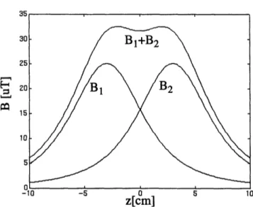
An obvious approach to improving the spatial characteristic of the surface coil configuration from the previous section, is to use a second wire loop a dis-tance apart from the first one, with the current in the same direction. The B field between the wire loops shows less fluctuation than with the single loop coil. This configuration is depicted in the next figure:

z d x wire loop 1 y wire loop 2

Fig. 13: Two current rings form a Helmholz coil

We can use EQ57 and the principle of superposition to get an idea about the field inside these two wire loops. Fig. 14 shows the field intensity for two wire loops separated by 6cm. Note that this is the plot of the intensities along the z

Fig. 14: Flux density profile for the Helmholz coil

axis. (i.e. x=y=O) For intensities with x, y O0 the field has even larger humps than depicted in Fig. 14. Stretching the coil along the y axis would certainly improve the situation for y 0 . That would result in a setup depicted in Fig.15:

z

Since all the current intensities I0 are the same we could connect the wires above in the right way to get a setup which is known as the saddle coil. This design must have a better field distribution than the two wire loop setup, but that the humps along the x and z axis are still apparent. A setup with more than 4 wires and different currents Io, would improve the B field characteristic fur-ther.

The saddle coil, as we will see later, can be viewed as a 6 mesh Birdcage reso-nator. A Birdcage resonator is simply a ladder network which is wrapped around a non metallic cylinder[2]. Fig.16 illustrates this:

ZL

ZR

"legs" of bird cage

Fig.16: A cylindrical ladder network is a Birdcage resonator

The object to be measured is located inside the resonator. The complex imped-ances ZL and ZR represent either lumped elements or distributed impedimped-ances or both. In most cases the "legs" of the Birdcage are simple wires or thin shims. Then a part of ZL would count for the inductance of this wire or shim.

It is important to note that ZR and ZL are not necessarily lumped elements, they represent the physical construction of the Birdcage. The currents through each of the legs contribute to the overall magnetic field distribution according to the superposition principle.

Resonance frequencies of the Birdcage resonator

Our objective in this section is to find an expression for the resonant fre-quencies of the Birdcage from which we can then find the leg currents that cre-ate the magnetic field inside the resonator. Two approaches will be used. First we derive the currents from Kirchhoff's laws with the appropriate boundary conditions and then we will compare it to a transmission line approach [2]. Of course the two methods should deliver the same results.

iI (ii)

7: Equivalent for a Birdcage resonatorcircuit

Fig. 17: Equivalent circuit for a Birdcage resonator

3.3

The network in Fig. 17 represents the resonator which has been cut "in the middle" of impedance ZL at leg position N/2. N is the total number of legs. Note that the connection of the points labeled A and B yields the original reso-nator. Thus the impedances at point N/2 are twice as high as ZL. We recognize that the ladder network is symmetric and thus currents and voltages on the right side of leg 0 are the same as currents and voltages on the left side of leg 0. Therefore the indices used to determine voltages and currents can be applied on either side. Considering an initial current Io in the leg at position n=0, and using Kirchoffs relation:

EQ58

Vk =O ,

Ik

=O

k k

We can see that J0 = -Io/2 . Assuming the knowledge of ZLand ZR and

using Kirchhoffs voltages law we can write: EQ59

IOZL- 2JOZR - I ZL = 0

and EQ60

J1 = Jo- II

Combining EQ59 and EQ 60 yields: EQ61

I = Io 1 +

and EQ62

Ji = -Io +

for-mulae can be obtained by applying Kirchhoffs law to the next meshes using the knowledge of the previous currents. This yields the following recursive equations:

EQ63

In + 1 = I-2Jn

ZL

Jn+ 1 - Jn-In+ l

Substituting k = ZR/ZL and carrying out the above recursion, the currents In and Jn can be expressed as a polynomial in k

EQ64 I n Jn (k) -2 dni i=O n In (k) = o cniki i=O

Appendix A shows how to calculate the coefficients ciand di . At this point, it

is only important to note that the current in each leg can be represented by a polynomial function and the coefficients can be computed. The argument of the polynomials (i.e. k) is directly related to the impedances ZR and ZL (i.e. ZR/ZL). Thus the polynomials are totally independent of the physical con-struction of the Birdcage. The only constraint is that ZR and ZL are equal in every section of the resonator. Notice that the Birdcage is still "open" i.e. the ends of the ladder network of Fig. 17 have not been connected yet and N (the number of legs) is still undetermined. Before reconnecting the resonator, we have to account for the doubled impedances at the end of the ladder, for the calculation of the polynomial functions IN/2(k) and JN/2(k). Appendix Al

Define positive indices for currents and voltages on the right side of the ladder network in Fig. 17 and negative indices for voltages and currents on the left side. By Defining Vn as the potential voltage between two impedances ZL and

due to symmetry it follows that: EQ65

Vn = V n

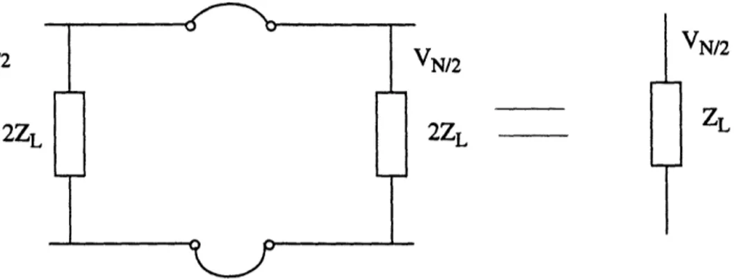
and consequently this has to be true for n=N/2 and n=-N/2. Now consider to connect the points A and B (i.e. closing the ladder network to get the original Birdcage). Fig. 18 depicts this "closing procedure"

2 VN/2

N/2

22L

--

lz

Fig. 18: Reconnecting the ladder network to yield original Birdcage

From EQ65 we know that the two potentials VN/2 and VN/2 are equal. Thus we can say that the currents JN/2 and J-N/2 have to be zero. This applies a

boundary condition to the polynomials which represent JN/2 and J-N/2 i.e.:

EQ66

JN/2(k) = J-N/2 (k) = 0

Since this polynomial has the order N/2, a maximum of N/2 roots are possible i.e. only N/2 k values satisfy EQ66. No information has been given about

ZR and ZL, thus EQ66 is valid for any N mesh Birdcage resonator.

V-N/2

Considering a low pass Birdcage (i.e. a resonator with inductive ring elements and capacitive leg elements) with known parameters ZR and ZL and assuming the most simple model (i.e. the ring impedance is a pure inductor

ZR = jL and the leg impedance is a pure capacitor ZL = -j/ (OC) we

can express k as: EQ67

k

=

Since k is restricted to N/2 distinct (kl,k2,k3,..kN/2) values and L and C are

constant (i.e. the physical inductors and capacitors of the resonator), the boundary conditions of EQ66 can only be met if the frequency w is:

EQ68

j=

LC

where kj are the roots of JN/2(k). The roots are certainly the same on the right

and left side of the ladder network and can be viewed as a two fold degeneracy [3]. In section 3.3 we will use numerical methods to verify the resonance fre-quencies of this particular Birdcage..

This simple resonator has been described earlier [2] with a transmission line model. The results of the two approaches are compared.

The resonance frequencies in [2] are: EQ69

2 . rM

Co = sin

J7I

N'

where M corresponds to the mode (i.e. j in our notation), L1 is twice the ring

inductance of one segment of a low pass Birdcage (i.e. L in our notation), N the number of legs and C the value of the leg capacitor.

EQ68 and EQ69 should yield the same resonance frequencies since the same elements are assumed. (i.e. ring impedances are inductors with value L = 1/

2L1 and leg impedances are capacitors with value C)

Changing EQ69 to our notation (i.e. L₁= 2L) yields: EQ70

2

Oi=

-LC

N

Note that j refers to the mode as in EQ68. Comparing EQ68 and EQ70 yields: EQ71

A2 sin N = V/kj

A verification of EQ71 can be done by using the values for kj from Appendix Al for the 12 mesh Birdcage (i.e. N=12). The following table shows the results:

Table 1:

Verification of polynomial approach by comparison with transmission line

approach of Hayes et al 1 mode j /2 sin 1 0.3660 0.3660 2 0.7071 0.7071 3 1.0000 1.0000 4 1.2247 1.2247 5 1.3360 1.3360 6 1.4142 1.4142

The polynomial approach seems to be a little more complicated than the sim-ple sine function from Hayes et al [2]. The concept however can be used for any kind of leg and ring impedances and is therefore more general.

In order to get a reasonable RF field homogeneity it is advisable to design Birdcages with more legs. As a consequence, adjacent meshes are spatially close and therefore coupling between the leg wires may exist. An inductance that models the self and mutual inductances of the legs can be added to get a more exact model of the Birdcage. This is suggested in [2] but there is no fol-low up. In [3] the model for the mutual inductance has been included and the resonance frequencies are obtained by solving an eigenvalue problem. Here again the polynomial approach should yield the same result.

The new Birdcage model changes the leg impedance ZL to a series LC circuit: EQ72

ZL =j(OL - )

where L1is the inductor which models the self and mutual inductance of the

legs. The ratio ZR/ZL = k changes to:

EQ73

k

o02_L 1C- 1

Remembering that the boundary condition for JN/2(k) yields N/2 solutions for k and thus N/2 resonance frequencies. EQ73 can be solved for o,

EQ74

I C L kj

Since kj is the same for any N mesh resonator, introducing Llresults in a shift of resonances to higher frequencies, which is consistent with [3].

3.3.1 Birdcage design procedure including mutual inductance

From a practical perspective, it is rather difficult to exactly measure the inductances of L and L1. This knowledge, however, is needed to predict the

resonance frequencies with EQ74. Since it is much easier to measure the reso-nance frequencies of a Birdcage, the resoreso-nance spectra can be used to deter-mine L and L₁. Solving EQ74 for L and L1yields,

EQ75 L=2 1 2 o2Ct 02 (k2 - k) 'i EQ76

kLoD

- k

2

L

=

where k1 and k2 are any two roots of the polynomial JN2(k), o and o02the

corresponding measured resonance frequencies.

Since the capacitor values C are easy to measure, the following low pass Bird-cage design procedure is applicable:

1.Construct an N mesh low pass Birdcage with arbitrary capacitor value

Cstart.

2.Measure the N/2 resonance frequencies

4.Use EQ77 (derived from EQ24,EQ25,EQ26) to determine Cd for the desired frequencycod and desired mode m:

EQ77

-k O 2

C =Cm 1 9

d startd [k1(a - 1) -kma]

with the variable a defined as: EQ78

k 0) - k )2

a

-2 (k-2-kf)

3.3.2 Comparison of polynomial approach with [3]

As a verification of the polynomial approach (including the leg inductors) we use the resonance frequencies obtained by [3].

His resonator is a 8 mesh low pass Birdcage and his equation [6] for the reso-nant frequencies is:

EQ79

oj2 = 22 [1 - cos (2iEj/N)] / [ 1-2 (a/Cb) 2_{cos2; (j/N) ]}

where 20a is the resonance frequency of a single mesh and cob is the reso-nant frequency of a single leg. coa and cob have to be adjusted to yield the 4 resonant frequencies observed by the experiment ([3] page 53)

for j=2 EQ79 reduces to EQ80

CO2 = 22

EQ81

2CO2cos (r/4)

_2 (

1

Using the calculated frequencies col and 0)2 ([3] page 53), EQ80 and EQ81 (which are derived from his equation [6])the following resonant frequencies are calculated:

Table 2:

resonant frequencies calculated with Tropp's equation [6]

i fj [MHz]

1 34.7

2 54.5

3 63.0

4 65.3

With the parameters coa and cob we can extract the inductance of the ring inductor and the mutual inductance between the legs ([3] page 52)

EQ82

M

l/C2,

EQ83

L = 1/(20aC)-M

where M is the mutual inductance between the legs, L the inductance of the ring inductor and C is the given leg capacitor with value 62pF. Note that in the polynomial approach we used the variable L1to express the mutual inductance

At this point we have determined the resonant frequencies w3and (04, the

ring inductances and the mutual inductances for a 8 mesh low pass Birdcage with the method proposed in [3].

Now the polynomial approach is used to determine the resonance frequencies of the same 8 mesh low pass resonator. It is sufficient to show that with the same physical parameters (i.e. leg capacitor C, ring inductor L and mutual inductance M) the polynomial method yields the same resonance frequencies. First we need to find the polynomial J4(k) of the 4 mesh ladder network with

the same procedure as we did it for the 12 mesh Birdcage example in Appen-dix Al. Executing the procedure and applying the boundary condition yields: EQ84

J4(k) = 8k4 + 40k3 + 68k2 + 44k + 8 = 0

The solutions of EQ84 are:

Table 3:

roots of J4(k) for 8 mesh Birdcage

j kj

1 -0.2929

2 -1.0000

3 -1.7071

4 -2.0000

Again, these roots are the same for all 8 mesh Birdcages no matter what impedances we use. The system is constrained to a low pass Birdcage by defining ZR = jo)L and ZL = jO)M + 1/ (j0C) . Using the parameters cal-culated from [3] (i.e. L, C, M) and applying EQ74 yields the resonant frequen-cies using our method.

nota-tion. Table 4 shows the results:

Table 4:

resonant frequencies using polynomial approach

i fj [MHz]

1 34.7

2 54.5

3 63.0

4 65.3

By comparing table 2 and table 4 exactly the same results.

we can see that the two methods yield

Additional initial conditions

The derivation of the N/2 resonance frequencies in the previous section is based on the assumption that the current I is present at leg 0. With this initial condition, we derived the resonance frequencies for a general Birdcage. Let us use the same concept to derive the resonance frequency of a simple parallel circuit of two pure imaginary impedances Z1and Z2as shown in Fig. 19.

Z1 Z₂

Fig. 19:

parallel circuit to show concept of high impedance mode 3.3.3

As we did for the Birdcage we assume a given current Io and apply Kirchhoffs law again:

EQ85

10(Z1+Z2) = 0

Using the substitution Z1/Z2 = k we get:

EQ86

Io(k+l) = 0

which can be viewed as a polynomial in k of degree 1. The solution of course is k1 = -1 . If Z1 is a capacitor C and Z2 an inductor L we get:

EQ87

Z1 1 ₁

Z2 o2LC

which yields of course the resonance frequency of a parallel LC circuit. Since the system is resonating unperturbed (i.e. no energy is dissipated) it can be viewed as a high impedance (infinite resistance) circuit. This parallel LC cir-cuit example should make clear, that the assumption of the initial current IO yields the high impedance resonance frequency. Therefore the derivation of

the Birdcage resonant frequencies in the previous chapter yields high imped-ance modes.

If we now reconsider the transmission line model, we know that it acts as a low impedance at certain frequencies. (i.e. reflection factors of -1) This is eas-ily shown by considering EQ34 in chapter 2.2.6:

EQ88

V

r (z) = VtSe2yz

Consider the position

z to be fixed and the complex propagati

Y = j[ = jo/v the reflection as a function of frequency is, EQ89

(

o)

where v is the phase velocity.

Clearly EQ89 crosses low and high impedance points (i.e. -1 and 1) in the complex reflection plane as a function of the frequency cO . Since the ladder network which models the Birdcage is similar to the transmission line model of Fig.2, we can intuitively conclude that the Birdcage must have resonant fre-quencies which correspond to low impedances or, with the LC analogy, series resonant modes.

Let us again consider the ladder network in Fig. 17. If the input impedance across the leg impedance at position 0 has to be zero (corresponding to a reflection factor of -1), then there is no current present in leg 0. Therefore the initial condition is,

EQ90

o = o0

and with connecting a current source across leg 0 EQ91

1

JO=

0 2

Note that Jo can be any constant since the roots of the polynomials are not affected by a constant multiplier. Here we use 1/2 for convenience. With these initial conditions we use EQ63 again to recursively compute the coefficients for the J and I polynomials. The resulting coefficients are shown in Appendix

A2.

'high impedance' case, yields the ring current JN/2- Applying the same bound-ary condition as before (i.e. JN/2=0) for a 12 mesh Birdcage we get:

EQ92

J6(k) = (32k6 + 192k5 + 432k4 + 448k3 + 210k2+ 36k + 1) = 0

The k values which satisfy EQ92, shown in Appendix Al, are related to the frequencies with zero input impedance (and hence the name low impedance resonance frequencies).

The conclusion therefore is that an N-mesh Birdcage resonator has a total of N resonance frequencies, i.e. N/2 high impedance and N/2 low impedance reso-nances. The selection of either mode can be done with the matching circuit. (as in the case for parallel and serial LC circuit; see chapter 2.3)

3.4

Current distribution

The RF-field distribution inside the bird cage resonator is a superposition of the induced magnetic field due to the current flux through each individual leg. (see 3.1) In order to compute the magnitude and phase of this field, the currents must be known. We have already derived an expression for these cur-rents In in order to arrive at the resonance frequencies (i.e. the polynomial

functions in

ZR/ZL)-Each polynomial In represents the current flux through the leg at the angular

position 27n/N , where n is the leg number and N the total number of legs as shown in Fig.20.

leg

Fig.20:

Definition of angular position p

Suppose we express the current as: EQ93

In = 10u(np)

where u(x) is an unknown function of the current distribution and (p is 2/N (with N the total number of legs).

From EQ61, the current through the first leg (I1) is EQ94

I1 = Io(1 +k).

Applying EQ93 to the first leg and combining combine EQ93 and EQ94, EQ95

Io (1 +k) = Io (u(p)

Solving EQ95 for k yields, EQ96

Note the index i is introduced since we know that only N/2 k values and thus N/2 distinct unknown functions are possible. Replacing kiin EQ64b (i.e. the

polynomials for the leg currents) with EQ96 yields to the following set of polynomials:

EQ97

u_i(0) = 1

ui(q)

= l +

(ui()-

1

)

ui(2qo) = +4(ui(p)-1)

+2(ui(9p)-1)

ui(3(q) = 1 +9(ui((p) -1) + 12(ui((p) - 1)

_{+4(ui((p) -1)}

Expanding and rewriting yields: EQ98 Ui() = 1I ui((P) = i (() Ui(2q0) = - 1 + 2u (p) ui(3qp) = - 3ui ((p) + 4u3₍₎ ui(4(p) = 1 - 8u (p) + 8u4 (p) or EQ99 n

ui(ny) = ,al[u() ]l

Cheby-chev polynomials[9]. They are defined as: EQ100

Tn(x) = cos (n(p) with x = cos ((p)

The Chebychev polynomials can be derived from the identity[9]: EQ101

cos ((n + l)(p) + cos ( (n - 1)(p) = 2cos ((p) cos (n(p)

The coefficients in EQ100 are equivalent with the coefficients obtained in EQ98. Thus unknown functions ui(P) must becos (ip) .

for i=1..N/2.

By summarizing above steps the leg current distribution for a Birdcage tuned to the high impedance modes is,

EQ102

In= Icos (nqp) with (p 27m

where N is the total number of legs and m = 1..N/2.

The concept of splitting the leg impedance at leg position N/2 and using the boundary condition JN/2(k)=O, implies that the leg current distribution must be

an even function around N/2.

What is the current distribution when the Birdcage is tune to the low imped-ance mode?

In this mode the current through the first leg is zero and that the current distri-bution function has to be even around both the first leg and the leg at N/2. (symmetry argument) Let us now consider a given current IN/2 at leg position

N/2. If we split the resonator at this position, we are left with half of IN/2 and a

doubled leg impedance. Fig.21 illustrates this:

VN/2 ZL IN/2 VN/2 2_ZL V-N/2 2_ZL 1/2 IN/2

Fig.2 1: Splitting of leg at N/2 to show current distribution in low impedance mode

With the N/2 mesh shown in Fig.22:

ZR ZL IN/2-1

I

I

Fig.22: Mesh at leg N/2

Writing down Kirchhoffs law: EQ103 IN/2ZL-2ZRJN/2 -IN/2 -1 ZL = 0 I

c

and JN/2 = we get: JN12 -2 N/2 EQ104 IN/2- = _IN/ 2 ( 1 k) and EQ105 JN/2 = IN/2(

+ k

EQ 104 and EQ 105 are equivalent with EQ61 and EQ62 except for 'backwards running' indices. Therefore the same recursion can be applied and the same

polynomials as in EQ64 result (except the n index). Thus we can write, EQ106 N/2 -n In (k) = 2 2 CN/2n i k i i=O N/2-n Jn (k) = 2 E dN2-n,i i=O

where the coefficients cniand dniare shown in Appendix Al.

We can now use the zero current in the first leg as the boundary condition. Doing this yields a set of k values which satisfy this boundary condition. For a 12 mesh Birdcage these k values are identical with the ones calculated in Appendix A2.

In the previous section we have shown that the evaluation of the polynomial at leg position n yields a cosine function.

For the low impedance modes we have shown that the same polynomials can be used if the starting point of the recursion is N/2. Thus the current distribu-tion has to have a cosine shape starting at N/2. Since the zero current con-straint has to be met for the first leg the current distribution function has to be

IN/2COS ( [N/2-i] (p/2) with i being the leg number and ( = 2/N

This expression can be written as, EQ107

Ii = -IN/ 2sin 2

i)

Since we have again N/2 polynomial roots which meet the boundary condi-tions we get the set of low impedance current distribution funccondi-tions by using EQ107 with (p = 2cm/N where m is an integer from 1...N/2.

3.5

Numerical methods

The analytical description of the Birdcage derived in the previous sections, provides a basic understanding of how the resonator works. However all the derivations are made with the assumption of symmetry i.e. all components have the same values and the leg and ring spacings are equal. The numerical tools described in this chapter simulate a Birdcage numerically. This allows a verification of the previous analytical derived results and provides some insight of the non symmetric case. A particular example of a low pass

Bird-cage which will be shown and will be constructed later (chapter 3.4). We use two numerical methods to compute resonant frequencies and current distribu-tion for this example. The element values have been chosen to yield approxi-mate resonance frequencies in the range of 10-100MHz.

PSpice computation

The first numerical tool is a electrical analysis program called PSpice. The input of this software package is a list with all the elements used, combined with an instruction set of how to connect them. Further, the experiment to be performed on the circuit and the format of the result have to be defined. As a first step, Birdcage has to be designed. This is illustrated in Fig.23

L12 rFV'Y L1 _L2 C1 11 L7 C2 12 5 23 1,11 25 C3 L8 13 29 L24 111 L23 49 51

Fig.23: LC network with node labels for Spice analysis

Note that every node is labeled with a number that is used to instruct PSpice how to connect the elements. This example is a 12 leg Birdcage. Appendix B shows the script to perform a frequency response analysis. As a first experi-ment the leg inductors have been set to zero. The program has problems with 3.5.1. 1 II - -:Cll L -,

pure imaginary numbers near the resonance frequencies since the currents and voltages approach infinity. Adding small resistors in series with the reactive elements solved this problem.

The voltage source is connected via a resistor to the first leg. For the high impedance resonant modes, the voltage at node 2 should approach the value of the voltage source (i.e. V0) and for the low impedance modes the voltage at

node 2 should be zero. The next figure shows the frequency response at node 2 for a low pass Birdcage with ZL = -j/oC ,C=55pF and ZR = joL,

L=68nH.

0 20 40 60 80 100 120

freq [MHz]

140

Fig.24: Spice frequency rersponse

J

-Using the same terminology as in the analytical derivation, we can say that the zero points correspond to the series resonant modes and the points where the node 2 voltage approaches 1 correspond to the parallel resonant modes. This is in agreement with the N resonance frequencies derived analytically.

Using the same leg and ring impedances, the resonance frequencies are calcu-lated analytically:

a) high impedance resonant frequencies:

from Appendix Al we get the 6 solutions of J6(k):

Table 5: k solutions for 12 mesh bird cage -2.000 k5 -1.866 k4 -1.500 k3 -1.000 k2 -0.500 kl -0.134

Using the simple model quencies are defined as, EQ108

discussed in chapter 3.3 where the resonant

fre-i---

LC'

yield,

Table 6: high impedance resonant frequencies for 12mesh Birdcage example

res freq MHz c06 116.39

Table 6: high impedance resonant frequencies for 12mesh Birdcage example

(04 100.79

03 82.30

°02 X58.19

co1 30.13

These resonance frequencies are equivalent with the frequencies observed with the PSpice frequency plot at the points where the graph approaches 1.0 in Fig.24

b) low impedance resonant modes

Similarly we use the roots (from Appendix A2) for the low impedance

polynomial J6(k) to compute the second set of resonant frequencies.

Table 7: low impedance resonant frequencies for 12mesh Birdcage example

0)6 115.39 0)5 107.53 (04 92.33 o3 70.85 (02 44.54 01 15.19

These frequencies correspond to the zero points in the PSpice output plot.

The PSpice calculation and the analytical solution for the resonant frequencies yield the same values for a 12 leg low pass Birdcage example as expected.

3.5.2 MATLAB computation

The second method uses the program MATLAB which is a widely used pack-age to perform general numeric calculations. A recursive function performs an impedance calculation as a function of frequency. To see how the algorithm works, let us again consider the Birdcage ladder network where the leg at N/2 is split.

I]

i_

Fig.25: Equivalent circuit for a Birdcage resonator

First consider only one half of the network. Define the impedance at N/2 Zinit.

Zinit has the double value of the leg impedance ZL due to the splitting of the resonator at position N/2. A MATLAB function, with Zinit as input parameter, is called to compute the last mesh i.e. a parallel circuit calculation of

ZLH (2ZR +-Zinit) to yield a complex impedance Ztmp. Ztmp can now be entered into the same function (i.e. as Zinit of a N-1 leg resonator) This recur-sion is repeated N/2 -1 times. With the last call of the routine (i.e. when N=1) the network has "shrunk" to an equivalent circuit shown in Fig.26.

Iiz

I ZR ZR

Zinit ZL Zinit

ZR ZR

Fig.26: Birdcage compressed with recursive function

The series circuit of Zinit and 2ZR yields the total impedance of one side of the resonator without considering ZL (define Z'=Zinit+2ZR). Since we are inter-ested in the impedance of the whole resonator and the left and the right side are identical we conclude that the total impedance without the center ZL is Z'/ 2. Therefore the last recursion call computes ZL// [ (2ZR + Zini) /2] which is the total impedance of the Birdcage resonator.

We can define a frequency vector to compute the total impedance as a function of frequency. Fig.27 shows the frequency response.

x10S

20 40 60 80 100 120 140

-irsa f[MHz]

Fig.27: resonance frequencies using the recursive method

3 A 2.5 Ztot 2 1.5 1 0.5 cl

Note that the intensities of the peaks vary since a discrete set of frequency points is used to determine the impedances. The impedance values at the high impedance resonance frequencies is infinity, sampling between these points yields the observed variation.

Expanding the y axis of Fig.21 reveals the position of the low impedance reso-nance frequencies. This is shown in Fig.28.

,n-&u 8 6 4 2 0 20 40 60 80 100 120 140

Fig.28: Expansion of Fig.27 to see low impedance resonance frequencies Note that the position of the peaks and the valleys in Fig.27 and Fig.28 are identical with the resonance frequencies derived analytically and listed in table 6 and table 7.

Fig.29 shows the structure of the recursive function calc_bg. function calcbg(N,Zinit)

N>1?

Y n

calc_bg(N- 1 ,ZL//Zinit+2ZR) Zres=[(Zinit+2ZR)/2]IIZL

IF structure of recursive functionig.29: Fig.29: structure of recursive function

In appendix C a listing of the above recursive function can be found.

This recursive numerical method is considerably faster than the approach with the PSpice program for the same number of frequency samples and there is no need to add small resistors.