Bayesian Approaches to Bilinear Inverse Problems
Involving Spatial Evidence: Color Constancy and
Blind Image Deconvolution
by
Barun Singh
Submitted to the Department of Electrical Engineering and Computer Science
in partial fulfillment of the requirements for the degrees of Engineer of Computer Science
and
Master of Science in Electrical Engineering and Computer Science at the
MASSACHUSETTS INSTITUTE OF TECHNOLOGY
June 2006@
Massachusetts Institute of Technology 2006. All rights reserved.A uthor ... . ...
Department of Electrical Engineering and Computer Science
26, 2006 Certified by ...
William T. Freeman
-ingisor
Accepted by....- nith
Chairman, Department Committee on Graduate Students
BARKER
MASSACHUSETTS INSMTT-JTOF TECHNOLOGY
Bayesian Approaches to Bilinear Inverse Problems Involving
Spatial Evidence: Color Constancy and Blind Image
Deconvolution
by
Barun Singh
Submitted to the Department of Electrical Engineering and Computer Science on May 26, 2006, in partial fulfillment of the
requirements for the degrees of Engineer of Computer Science
and
Master of Science in Electrical Engineering and Computer Science
Abstract
This thesis examines two distinct but related problems in low-level computer vision: color constancy and blind-image deconvolution. The goal of the former is to separate the effect of global illumination from other properties of an observed image, in order to reproduce the effect of observing a scene under purely white light. For the latter, we consider the specific instance of deblurring, in which we seek to separate the effect of blur caused by camera motion from all other image properties in order to produce a sharp image from a blurry one. Both problems share the common characteristic of being bilinear inverse problems, meaning we wish to invert the effects of two variables confounded by a bilinear relationship, and of being underconstrained, meaning there are more unknown parameters than known values. We examine both problems in a Bayesian framework, utilizing real-world statistics to perform our estimation. We also examine the role of spatial evidence as a source of information in solving both problems. The resulting blind image deconvolution algorithm produces state-of-the art results. The color constancy algorithm produces slightly improved results over the standard Bayesian approach when spatial information is used. We discuss the properties of and distinctions between the two problems and the solution strategies employed.
Thesis Supervisor: William T. Freeman
Acknowledgments
Thanks go first and foremost to my advisor, Bill Freeman. Not only were his insights and assistance critical in helping me conduct the research presented in this thesis, he was also particularly understanding of the fact that life can take myriad twists and turns that set you on new and exciting paths. He allowed me to make the most of my MIT graduate experience and I doubt most advisors would have been so supportive. Thank you to all of my colleagues who have answered so many questions and helped me learn much more about computer science through casual conversations than I could have through any class. In particular, Marshall Tappen has been my officemate for the last four years and a great person to ask questions, discuss ideas with, and debate.
The deblurring research that constitutes about half of this thesis was conducted jointly with Rob Fergus, without whose tireless efforts that work likely would never
have seen fruition. It was great to be able to work with him on the project.
The time I have spent in the AI/CSAIL lab has been made particularly enjoyable
by all of the great people I get to interact with on a day-to-day basis, not just within
my research group but also the other vision and graphics groups. More generally, I have had the fortunate opportunity to become friends with some spectacular people throughout this Institute and to all of you, I say thank you for being part of my life.
I will always owe my family, my mother and father in particular, an enormous
debt of gratitude for all of the sacrifices they have made for me, for teaching me, and for guiding me so that I would have the opportunities I have today.
Words aren't anywhere near adequate to express my deep appreciation for my wife, Sara. Her intense love and support has seen me through the most difficult times in my life, and has made every day we're together seem like a blessing. Thank you, thank you, thank you.
This thesis is dedicated to my brother, Bhuwan. He lived his life filling the hearts of everyone around him with love, and left this earth far before he should have. I always looked up to him, and I can only hope to one day live up to the memory he has left behind.
During the time this research was conducted, I have been supported by the National Science Foundation, Shell Oil, the National Geospatial Intelligence Agency NGA-NEGI, the Nippon Telegraph and Telephone Corporation as part of the NTT/MIT Collaboration Agreement, and the MIT Office of the Dean for Graduate Students Ike Colbert.
Contents
1 Introduction
1.1 Color Constancy . . . . 1.2 Blind Image Deconvolution . . . .
1.3 Spatial Characteristics of Natural Images . . . .
1.4 Outline of Thesis . . . .
2 Bayesian Methods
2.0.1 Probability Distributions . . . . 2.1 Estimation by Minimizing the Bayesian Expected Loss . . 2.1.1 Implementation and Local Minima . . . . 2.2 Variational Bayesian Approach . . . .
2.2.1 Probability Mass Versus Probability Value . . . . . 2.2.2 Implementation . . . .
3 Color Constancy
3.1 Standard Problem Formulation . . . .
3.2 Related W ork . . . .
3.3 Hyperspectral Data . . . . 3.4 Using Spatial Information: Spatio-Spectral Basis Functions 3.4.1 Characteristics of Spatio-Spectral Basis Functions . 3.4.2 Reducing the Number of Parameters . . . .
3.5 Bayesian Color Constancy Using Spatial Information . . .
3.5.1 Choice of Probability Models . . . .
3.5.2 Implementation Issues . . . .
3.6 R esults . . . .
4 Blind Image Deconvolution
4.1 Related W ork . . . . 9 10 11 12 13 15 . . . . . 16 . . . . . 18 . . . . . 20 . . . . . 21 . . . . . 22 . . . . . 24 27 27 31 33 35 37 40 . . 42 42 43 . . 45 49 49
4.2 Problem Formulation . . . . 4.2.1 Image Formation Process . . . 4.2.2 Blur Process . . . . 4.2.3 Image Model . . . . 4.3 Blur Kernel Estimation . . . . 4.3.1 Choice of Probability Models 4.3.2 Variational Bayes Estimation 4.3.3 Coarse-to-Fine Estimation 4.3.4 Inference Algorithm Details 4.4 Blur Removal . . . . 4.5 Complete Deblurring Algorithm . . .
4.6 Results . . . .
5 Discussion
5.1 Estimation Techniques . . . . 5.2 Prior Probability Models . . . . 5.3 Use of Spatial Information . . . .
5.4 Conclusions . . . . . . . . 50 . . . . 50 . . . . 5 3 . . . . 56 . . . . 56 . . . . 5 7 . . . . 59 . . . . 6 1 . . . . 64 . . . . 6 5 . . . . 6 7 . . . . 68 81 81 82 83 84
Chapter 1
Introduction
We often take our ability to process visual stimuli for granted. In reality, however, images are very complex objects, and processing the information contained within them is a difficult task. The image formation process involves the characteristics of and interactions among the items in a scene, the light sources shining upon and within the scene, and the imaging device. Humans are able, for the most part, to separate out many or all of these effects into their component parts, an important step in being able to extract useful information from visual data. Examples of this include our ability to recognize objects within an image and ascertain their three dimensional nature, deduce the true shape and characteristics of objects in blurry images, differentiate between shadows and changes in material properties, determine the illumination-independent color of items in a scene, and so on.
Though it encompasses a number of sub-fields, most of computer vision can be thought of as ultimately seeking to replicate the abilities of the human visual system. It is often helpful to break down this general category of research into two sub-categories: low-level and high-level computer vision. Low-level vision problems are those that relate to the process of light being shone from a source, reflecting off a set of surfaces and being recorded by an imaging device, and how to understand the characteristics of that process. These often involve operations at the pixel or sub-pixel level. In contrast, a high-level vision problem involves understanding concepts about the scene being imaged, or objects within that scene. One can think of low-level vision as involving image processing, while high-low-level vision deals with image understanding.
Much of the challenge of solving a high-level vision problems is being able to define it in mathematical terms. For example, identifying how many cars are present in a given scene is intuitively obvious for people to understand, but defining some
mathematical notion of what a car looks like for use by a computer algorithm is very challenging. Low-level vision problems have a benefit over high-level problems in that they are usually very straightforward to describe mathematically. However, they are often very difficult to solve because nearly all of them are underconstrained. That is, there are more unknown parameters than there are known values. This thesis examines a particular class of underconstrained low-level problems known as bilinear inverse problems.
An inverse problem is one in which we observe some effect, and we wish to un-derstand the causes that led to that effect. In computer vision, the effect is generally the observation of a particular image, and the causes are some set of properties of the scene and image capture device. A bilinear problem is one in which the unknowns are related to the known value by a bilinear function, i.e. a function with two unknowns that is linear with respect to each variable if the other is held constant.
The simplest example of an underconstrained bilinear inverse problem is
y =ab, (1.1)
where we observe y and we wish to determine the values of the unknown variables a and b. Clearly, without any additional information, there is no way for us to obtain an answer, as there are two unknown variables and only one data point. We approach this sort of problem using Bayesian methods. Bayesian methods are built upon a probabilistic framework that allows us to incorporate statistical information about the world into our solution. In the types of problems we are concerned with, the unknown variables will represent properties of natural images, and as we will see, the statistics that govern these properties can provide very strong cues to solving low-level vision tasks.
This thesis examines in particular how statistics regarding the spatial configura-tion of natural images might help in low-level computer vision tasks. To do so, we consider two specific problems: color constancy and blind image deconvolution.
1.1
Color Constancy
Color is important in our understanding of the visual world and provides an effective cue for object detection and recognition. In general, however, the observed color of an object differs from its "true" color due to contextual factors such as lighting and orientation. An example of this can be seen in Figure 1 which shows the difference
between an outdoor scene as it would look under white light and as it actually appears at dusk. Color constancy refers to the ability to perceive the color of an object as approximately constant regardless of any such contextual factors. We are able to reliably use color for a variety of vision tasks largely because of our ability to perform color constancy well.
(a) Outdoor scene under white light (b) Outdoor scene at dusk
Figure 1-1: Example of an outdoor scene under two different lighting conditions. In performing color constancy, we wish to determine what a given image would look like under some canonical illuminant (white light). In this particular example, we would want to obtain the image on the left given the image on the right.
The color constancy problem, even in its simplest formulation, is inherently un-derconstrained. The image formation process consists of an illumination reflecting off of a surface, then being passed through a set of sensors. The input to the sensors is the product of the illumination spectrum and the surfaces reflectance spectrum. Different combinations of illumination and reflectance spectra can produce the same spectrum impinging on the sensor, and various sensor inputs can result in the same sensor responses. Due to these ambiguities, it is generally impossible to uniquely separate the effect of the illumination and the surface reflectances in an image. The goal of computational color constancy, therefore, is to optimally (under some metric) estimate either the reflectance and illumination spectra, or the effect of these spectra, at each point in the image.
1.2
Blind Image Deconvolution
Blind image deconvolution is used to restore images that have been corrupted by some stationary linear process. The corrupted observation is the result of a convolution between the original image and some unknown point spread function (PSF). Image deconvolution is referred to as blind if the PSF is unknown, and non-blind if it is known.
Corruption caused by an unknown PSF is common in a variety of imaging appli-cations, including astronomical and medical imaging. For natural images, the most common form of PSF is a blur kernel that is caused by camera shake during the image capture process (in which case the corrupted image is a blurry version of the original sharp image). An example is shown below in Figure 1-2. Camera shake is a signifi-cant problem for the average consumer-level photographer, particularly in situations where longer exposure times are needed to capture the scene because of low ambient light. In this thesis, blind image deconvolution will be synonymous with deblurring images that have been corrupted by camera shake.
(a) Actual (sharp) scene (b) Camera motion (c) Captured (blurry) image
Figure 1-2: Example of a blurry image caused by camera shake. Figure 1-2(a) shows what the image would have looked like if the camera remained still. The camera motion is shown in 1-2(b), where the magnitude of the grayscale value is inversely proportional to the length of time that the camera spent in a particular location. The resulting blurry image is shown in 1-2(c).
1.3
Spatial Characteristics of Natural Images
A great deal of recent work in computer vision has shown that images of real-world
scenes exhibit particular spatial characteristics that can be helpful in performing a wide variety of tasks. Although natural images do not obey well-defined distributions in terms of their absolute color values, there is a great deal of regularity in the distribution of their gradients and their responses to a variety of linear filters. In particular, these distributions are heavy-tailed; that is, they have most of their mass close to zero, but they also have some probability mass at large values as well. A Gaussian distribution, in comparison, would have much less probability mass at these large values. This property describes our intuitive understanding of natural images: they consist primarily of regions that are mostly "flat" or have slight gradients due to shading, interrupted occasionally by abrupt changes due to albedo, occlusions, or edges.
Heavy-tailed natural image statistics have been very useful in producing state-of-the-art results for many computer vision tasks, including denoising [40], superresolu-tion [43], estimating intrinsic images [46], inpainting [27], and separating reflecsuperresolu-tions
[26]. Encouraged by these results, this thesis explores if these types of statistics can
be utilized to achieve better results when applied to the problems of color constancy and blind image deconvolution.
- Empirical Distribution
0 Gaussian Approximation
2-8
-200 -100 0 100 200
Gradient
(a) A typical real-world image (b) Distribution of image gradients for the scene at left Figure 1-3: Example of heavy-tailed distribution in the gradients of a real-world image. The figure at right is shown on a logarithmic scale to emphasize the heavy-tailed nature of the distribution and its non-Gaussian nature.
1.4
Outline of Thesis
The remainder of this thesis is divided into four sections. The first of these gives an overview of Bayesian methods, introducing concepts and notation that are necessary in order to understand the remaining chapters.
The third chapter in this thesis discusses the color constancy problem in depth. This begins with an outline of the standard problem formulation and prior work. We then introduce the concept of spatio-spectral basis functions as a means of describing
spatial statistics. We present the results of color constancy when using these spatio-spectral basis functions, and find that for this particular problem, the use of spatial information helps to an extent in synthetic examples, and less so in real-world images. Chapter four deals with the blind image deconvolution problem. We again for-mulate the problem and discuss previous work. This is followed by an overview of algorithmic details involved in solving the problem, as well as a discussion of im-portant factors that must be considered and dealt with in order to achieve optimal performance. We present results for the application of deblurring images corrupted
by camera shake, showing that the algorithm provides state-of-the-art performance
for this application.
The final chapter discusses and compares the results of the color constancy and blind image deconvolution algorithms. In particular, we offer explanations as to why the use of spatial information assisted us in the case of deblurring but less so in the case of color constancy. We also compare the approaches utilized in solving both problems and describe inherent differences between the two problems that dictated the algorithmic choices made.
Chapter 2
Bayesian Methods
The work in this thesis relies on Bayesian methods. The primary characteristic of these methods is that they frame problems probabilistically and thus are able to produce solutions that incorporate a wide variety of statistical information, from the general characteristics of real-world processes to the assumed noise models for the particular problem at hand.
The probabilistic framework utilized by all Bayesian methods is based on three fundamental probability distributions - the prior, the likelihood and the posterior. Consider a problem of the form
y = f(0) + w (2.1)
where y is a set of observed data, 0 {Oij[1,nI} is a set of n unknown variables that describe the inner state of the system we are observing,
f(-)
is some known function, and w is a stochastic noise term that corrupts our observation. Our goal is to determine the inner state of the system 0 given a set of observations y.We model the system through its posterior probability, P(1y). The posterior is a mathematical representation of the probability that the internal state 0 takes on a specific set of values given that we make a particular observation y. It can be calculated using Bayes' rule as
11
P(AY) = P(y|6)P(0), (2.2)
Z
where P(yj0) is known as the likelihood, P(0) is the prior probability, and - is a normalization constant that is independent of the parameters to be estimated.
being estimated and the data. This includes both the functional relationship that maps the internal state to the observation in a noise-free environment,
f(-),
as well as the effect of the stochastic noise process.The prior, given by P(O), describes the probability that a certain set of values for
0 is the correct estimate without taking into account what we have observed. Any
constraints we have on the state variables (such as positivity or threshold require-ments) are described by the prior. This term also encodes the statistics we would expect 0 to observe in general (if we know nothing of these statistics, the prior will be uniform within whatever range of values 0 is allowed to take).
The posterior combines the information encoded within both the prior and the likelihood, and is the most descriptive model of the system available to us. Given the posterior probability, there are a variety of methods to obtain what may be considered an "optimal" estimate. These methods all rely on the notion of minimizing some cost function dependent upon the posterior probability, but differ in the type of cost function used.
2.0.1
Probability Distributions
Throughout this thesis, we will utilize several forms of probability distributions to describe the statistics of various image and scene properties. For the purpose of clarity, these distributions are described below:
Gaussian A Gaussian distribution, also known as a normal distribution, over a
random vector X is given by
G(XIL, E) = 1 exp (X - 1i)T -(X - /) (2.3)
where y E[X] and E = E[(X - p)(X - p)T] are the mean and covariance of X, respectively. Note that all of the terms multiplying the exponential can be combined into one normalizing constant, and we will generally ignore this constant and simply use the relation that
G(X1p, E) oc exp - (X - P)TE-1 (X - t)). (2.4)
In the case where X is a single random variable, y and E are both scalars.
Truncated We shall refer in this thesis to a truncated Gaussian distribution as a
Gaussian distribution over a random vector X that obeys the following:
(f
G( Xja b) ifO <AX +B <G(Trnc)(XIa, b, A, B) o 0 other e , (2.5)
0 otherwise
for some matrix A and vector B. Unlike the standard Gaussian distri-bution, none of the parameters of the truncated Gaussian distribution correspond directly to the mean or variance of the distribution.
Rectified A rectified Gaussian distribution shall refer in this thesis to a specific
Gaussian instance of the truncated Gaussian distribution in which we are dealing with a single random variable x, A = 1, and B = 0. This results in a distribution similar to the standard Gaussian distribution over a random variable except that it enforces positivity:
ReXp (- Zx - a)2 for x > 0
G(R)(xla, b) oc 2f - (2.6)
0 otherwise
Exponential The exponential distribution is defined over a random variable x as
{
A exp(-Ax) for x>00 otherwise
where A is known as the inverse scale parameter.
Gamma The gamma distribution is defined over a random variable x as
--E'-)x exp (- ax) for x> 0
Gamma(xja, b) () orwise (2.8)
0 otherwise
where a > 0 is the shape parameter and b > 0 is the scale parameter.
Mixture A mixture model does not refer to a specific form for a probability Models distribution. Rather, it refers to a method of combining many
distri-butions of the same functional form, known as mixture components, into a single distribution over the random vector X:
N
Mixture(X) = 7riP(XOj), (2.9)
where N is the number of mixture components being combined, 7ri is a weight assigned to component i, and Oi is the set of parameter values associated with component i, and
N
7r 1. (2.10)
i
P(X0j) may have any functional form so long as it is a valid
probabil-ity distribution and all mixture components have the same functional form (with different parameter values for each). In this thesis we will be using mixtures of Gaussians and mixtures of exponentials.
2.1
Estimation by Minimizing the Bayesian
Ex-pected Loss
The most common Bayesian estimation techniques operate by minimizing the Bayesian expected loss:
L ('l y) = OC (0, 0') P(0 1y)d6, (2.11)
Oopt = min L (O'l y), (2.12)
where C(0, 0') is a cost function that defines a penalty associated with a parameter estimate of 0' when the true value is 0, and 0opt is the optimal estimate.
Maximum a posteriori (MAP) estimation is one specific instance within this family of approaches in which
CMAP(0, 0') -6(0 - 0'), (2.13)
OMAP= max P(Oly). (2.14)
0
That is, MAP estimation produces the set of parameter values that, as its name would suggest, maximize the posterior probability. A very closely related technique is maximum likelihood (ML) estimation, which is equivalent MAP estimation under the assumption that the prior P(0) is uniform. In this case, the prior has no effect on the shape of the posterior, so that the set of parameters that maximizes the posterior are the same parameters that maximize the likelihood.
(MMSE) estimation, defined by the cost function:
CMAl SE (0, 0') = (0 _ 01)2. (2.15)
The value that minimizes the minimum mean squared error is the expected value of the probability distribution, OMAISE = E[0]p(oly).
Which of these techniques is best to use depends upon the problem being consid-ered. An advantage to the MAP solution is that it does not require any additional computation beyond knowing the posterior probability. However, there may not be a unique solution when using the MAP approach. This is often true in the case of underconstrained problems in which there are more unknowns than known values. For these problems, there may be an infinite number of solutions that explain the data equally well, and many of these solutions may have the same prior probability as well - hence, it is possible that there is not a unique set of parameter values for which the posterior probability is maximized.
Conversely, the minimum mean squared error estimate is in general unique but it is also computationally very expensive, requiring an integration over the entire posterior probability distribution for every point that is evaluated. An additional downside to it is that it can be very sensitive to small amounts of probability mass located at extreme points in the parameter space.
Other techniques that minimize the Bayesian expected loss have also been pro-posed, including maximum local mass (MLM) estimation, for which the cost functions is given by
CALM(0, O')= - exp(-KL (0 - 0)) (2.16)
and KL is set ahead of time. The MLM solution, like the MMSE estimate, requires an integration over the entire posterior probability distribution if computed exactly. However, good approximations exist which allow much more efficient computation that takes advantage of the fact that the MLM cost function only has non-negligible values in a very localized region [6]. The MLM estimate still requires more compu-tation than the MAP estimate, but it has the advantage that by taking into account the value of the posterior probability distribution in the region surrounding a certain estimate, it is more likely to provide a unique estimate without being affected by minor probability mass at the edges of the parameter space.
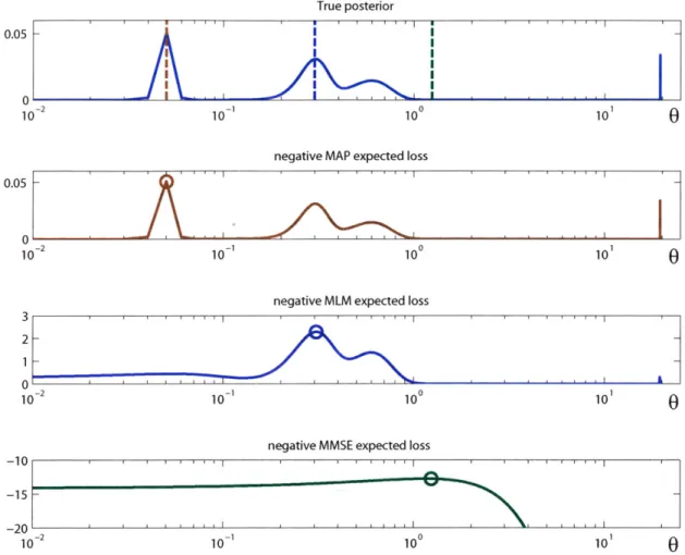
illustrates the differences between the MAP, MMSE, and MLM approaches. True posterior 0 1c 0.05 0 ic 3 2 1 0 -10 100 101
negative MAP expected loss
10 100 101
negative MLM expected loss
-210-1 10 0 10 1 0
A- 1
negative MMSE expected loss
10' 10 0 10 0
Figure 2-1: Example illustrating the effect of using different cost functions when minimizing the Bayesian expected loss. The top blue curve is a simple toy posterior probability distribution, as a function of a single scalar parameter 0. The three curves below illustrate the negative of the cost function being minimized when utilizing the maximum a posteriori (MAP), maximum local mass (MLM) and minimum mean square error (MMSE) approaches. The optimal solution is shown as a circle on these graphs, and the dashed lines on the top curve show the "optimal" estimate for 0 when using these methods. The x-axis for all plots is shown with a logarithmic scale in order to make the differences between the three methods more readily visible.
2.1.1 Implementation and Local Minima
In the discussion above, we have assumed that it is possible to find the true minimum of a given cost function. In reality, though, this can be very difficult. The form of the posterior probability is unknown, so finding the optimal solution for a given problem requires searching the entire space of 0 in order to evaluate the cost function at every
I I I I I I I I
IK-~
IA
I --0.05 - --15L -20 10point. In toy examples where 0 is one dimensional, such as the one illustrated in Figure 2-1, this may be possible. In real-world applications, however, 0 can often have millions of dimensions. Consider, for example, the fact that an average consumer-level digital camera produces an image with 4 million or more pixels. In a computer vision application, each of these pixels may have a unique 0, parameter associated with it (if we deal with color images, there may actually be three parameters for every pixel value associated with the red, green and blue color channels). In such a case, it is simply impossible to search the entire space of all pixels for the specific set of values that produces the maximum posterior probability, much less to evaluate a cost function at every point.
The construction of efficient algorithms for searching high-dimensional parameter spaces is a widely studied field of research. All existing approaches are, to some extent, still susceptible to local minima (or maxima). These local extrema are often characterized by strong nearby gradients that prevent search routines from being able to find more optimal solutions far away in the search space.
In real-world computer vision problems, the true posterior probability is generally plagued by many local maxima scattered throughout the search space. Initializations can play an important role in both the MAP and MLM approaches, and dimension-ality reduction methods, if they can be applied, may help. The MMSE approach, because it requires a global integration, is usually intractable in these applications. In the color constancy problem described in the next chapter, the problem is simply reformulated in a manner that greatly reduces the dimensionality of the search space (though problems of local minima can and generally do still exist even in this lower dimensional space).
2.2
Variational Bayesian Approach
An alternate way of looking at the maximum a posteriori approach described above is that it attempts to approximate the true posterior with a delta function, and the location of this delta function is the MAP estimate. Variational Bayesian methods
[1, 33] build upon this idea and instead seek to fit more descriptive functional forms to the true posterior, and apply the methods of the previous method to this functional form. This results in an approach that is sensitive to probability mass rather than probability value.
Let us denote by Q(0) an approximation to the true posterior probability distri-bution. The variational approach seeks to find the optimal approximation Qpt(0)
that minimizes the Kullback-Leibler (K-L) divergence, DKL, between the two
distri-butions:
Qopt() = min DKL (Q P) (2.17)
Q(O)
min Q(6) log dO. (2.18)
Q(O) fo P(O|y)]
The K-L divergence is a measure of the "distance" between two probability distribu-tions, and is non-negative with DKL(Q
IP)
= 0 if and only if P =Q.
Use of the K-L divergence has foundations in information theory, and DKL(QII)
can be described as the difference between the cross-entropy of P andQ and the entropy of P. In the
context of information coding the K-L divergence tells us the number of extra bits that must be transmitted to identify a particular value of a signal if the code being used corresponds to a probability distributionQ
instead of the true distribution P.In general, it is often desirable to obtain a single estimate for 0 as a solution. Because we know the analytical form of Q(0), marginalizing over the distribution becomes tractable. This allows us to calculate the mean of the optimal approximation, which is often taken to be the optimal estimate:
Oopt = E[Q(O)]. (2.19)
However, this need not be the case. The solution presented in Equation 2.19 is the
MMSE estimate over the approximate distribution Q(0). We may alternatively choose
to apply any of the other methods described in Section 2.1 to produce a single point estimate simply by replacing P(O1y) in Equation 2.11 with
Q(O).
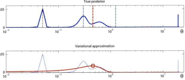
In this thesis we will be utilizing MMSE estimation in conjunction with the variational approach, so the optimal solution will be as defined above.Figure 2-2 shows the result of using the variational approach on the same posterior probability used earlier in Figure 2-1. In this example, a Gaussian distribution is chosen for Q(0).
2.2.1 Probability Mass Versus Probability Value
One of the primary advantages to the variational approach is that by fitting a distri-bution to the posterior it is able to describe where the probability mass is located, and the mean of the variational approximation provides the center location of this mass. This differs from the maximum a posteriori approach, which (in the ideal case)
0.05 0 Uc True posterior - -Variational approximation 0.05
--00
Figure 2-2: Example illustrating the effect of approximating the posterior probability with a Gaussian when using the variational approach. The top curve shows the same toy posterior probability illustrated in Figure 2-1. The light dashed lines are also the same as in Figure 2-1, illustrating the "optimal" estimate when using the MAP, MLM, and MMSE approaches. The thick dashed line shows the optimal estimate under the variational approach. This is identical to the mean of the approximate Gaussian distribution, which is shown in red on the bottom graph. Note that the Gaussian does not have the standard "bell" shape only because it is plotted along a logarithmic axis. The Gaussian is centered along the area of greatest probability mass of the posterior.
provides the single highest probability value location of the posterior. In general, describing the probability mass can oftentimes be more useful than describing the single point of highest probability.
The maximum local mass estimate is also more sensitive to probability mass than the MAP approach. However, the MLM technique is only sensitive to the probability mass in the local vicinity of a given value for the parameters, whereas the variational approach is sensitive to the probability mass of the posterior distribution as a whole. An alternate way of viewing the MLM approach is that it attempts to find the set of parameter values whose local vicinity is best described by a Gaussian with a pre-selected variance KL (as defined in equation 2.16). This is similar to the variational approach in the case where Q(O) is chosen to be Gaussian, except that the variational approach treats the variances as a free parameter to be estimated rather than a fixed value. Thus, the variational approach provides increased flexibility over the maximum local mass approach in order to find a more descriptive solution.
To illustrate how the MLM and variational approaches are related, suppose we run the variational Bayes algorithm using a Gaussian for Q(O) and a solution of
(Ovar, Kvar) as the mean and covariance of this Gaussian. If we then run the MLM
algorithm with KL = Kvar, we would get a solution of OMLAI = var. That is, the
optimal estimate under the maximum local mass estimate is identical to the mean of the variational approximation if the MLM variance is set to the variance of the variational approximation. In actuality, though, when running the MLM algorithm, we would not know what KL should be set to.
2.2.2 Implementation
As with the other techniques discussed in Section 2.1, there are limitations to what can be done with the variational approach in order to make it feasible to implement. We wish to produce a set of analytic update equations that can be used to optimize the settings for the approximate posterior distribution Q(O) (determining the values of these parameters through a search would be impractical even for small problems). In order to do this, we start with the assumption that the priors for each of our parameters are independent:
P(0) = JP(02). (2.20)
to the parameters:
Q(O) =JQ( 2). (2.21)
In this case, Equation 2.22 can also be rewritten as:
Q't (O) = Mil Q() log dO, (2.22)
= min jQ(0) log
(2)
dO, (2.23)Q(O> (o P(YjO)P(O))
=minf
Q(0j)
log(i
(02) dO, (2.24)Mi i Q(O) log
()
log P(yO) dO. (2.25)We can then marginalize over all but one of the parameters to get
Q't (j) = min Q(O ) [log Q(02) - log P(2) - (log P(yO))Q(ojo,)] dO1, (2.26)
Q(Oi) ,i (226
where (-) represents the marginalization operation, i.e.,
(log P(yO))Q(oIo) j Q(OIO)P(yjO)dO3 ,,gj. (2.27)
Solving equation 2.26 yields
QOPt (0i) + P(z) exp ((log P(y0))Q(oIoi)) , (2.28)
Zi
J
P(2) exp ((log P(yO))Q(olo,)) dO2, (2.29)where Zi acts as a normalizing term [33].
Equation 2.28 does not have a closed form solution. However, for particular forms of the prior probability, likelihood, and approximate posterior, iterative update equations may be derived that are practical to implement on real-world problems. These probability distributions must belong to the exponential family, as defined by
P(x) oc exp
(S
aifi(x)) . (2.30)There are only particular combinations of distributions in this family that will lead to iterative analytic solutions. Luckily, many of these combinations are practical for
use in real-world problems, and in Chapter 4 we will describe how the variational approach can be used for blind image deconvolution.
Chapter 3
Color Constancy
3.1
Standard Problem Formulation
Maloney [31] categorizes color constancy algorithms into two general forms: those that presuppose a "Flat World" environment and those that allow for a "Shape World" environment. The former class of algorithms do not account for the effects of geome-try, assuming that the true scene is flat. In this case, each point in the scene is fully described by a reflectance spectrum, a function only of wavelength. Any effects of geometry are folded into this reflectance spectrum. By contrast, the "Shape World" class of algorithms attempt to provide three dimensional models of the world, de-scribing each point in a scene using a bidirectional reflectance density function which is a function of wavelength and geometry. Such algorithms generally assume that something is already known about the geometry of the scene, and the models they utilize are not able to describe the complexities of real world scenes. In this work, we refer to color constancy in the context of the "Flat World" environment.
In order to frame the color constancy problem, it is first necessary to clearly articulate the process by which an image is formed. We assume that there is one uniform illuminant in the scene. All effects other than this uniform illumination are
considered to be due to the surface reflectances within the scene.
We assume image sensors that respond only within the visible range of 400nm to 700nm, and so are only concerned with the components of reflectance and illumination spectra that fall within that range. In order to make computations possible, we consider discretizations of these spectra, sampled at 10nm intervals to yield vectors of length 31.
prod-uct of the illumination and local reflectance spectrum. Let A index the discrete wave-length samples. For a surface reflectance S(A) and illumination E(A), the response at position x of a photoreceptor with a spectral response of Rk(A) is
y = Rk(A)E(A)Sx(A), (3.1)
where we have assumed zero sensor noise.
The illumination and surface reflectance spectra can be written as linear combi-nations of a set of illumination basis functions Ei(A) and reflectance basis functions
Sj(A), with coefficients ej and sj, respectively, at position x:
L E(A) =
Y
E(A)ej, (3.2) i=1 L Sx(A) = 5 Sj (A)sj, (3.3) j=1where L = 31 is defined as the number of elements in the A vector (i.e., the number of wavelength samples). Doing so allows us to write the rendering equation as
L L
y Z R(A) Ei(A)ei E SS (A)s>. (3.4)
Ai=1 j=1
Summing over A, we get a bilinear form,
L L
y = etGij,k sj, (3.5)
i=1 j=1
where Gi=,k Rk (A)Ei(A)Sj(A).
Given training data, principal components analysis (PCA) can be used to calculate the reflectance and illumination basis functions. An n-dimensional reconstruction of the training data using these bases is optimal in the sense that it provides the mini-mum mean-squared error between the actual data and its reconstruction as compared to any other n-dimensional reconstruction.
The number of basis functions used in the linear models of (3.2) and (3.3) are equal to the number of wavelength samples, so that the model fully describes the entire illumination and reflectance spectra exactly. In general, however, we wish to approximate the true illuminant E(A) and surface spectra Sx(A) using lower
dimen-sional linear models. Thus, we can define dE E(A) = E Ei(A)ej, (3.6) i=1 ds Sx(A) = Sj (A)sj, (3.7) j=1
where dE is the dimensionality of the illuminant approximation E(A), ds is the di-mensionality of the surface approximation Sx(A), and 0 < (ds, dE) < L. We now
decompose (3.5) as:
dE dS dE L L ds L L
yZ eGij,ksZ + eiGi,s
>+
> eiGi,k s+>
e.Gi,k sji=1 j=1 i=1 j=dS+1 i=dE 41 j=1 i=dE41 j=dS41
dE ds
= e Gjj,ksj +Wk,
i=1 j=1
(3.8)
where wx is the aspect of the sensor response that is not described by the lower dimensional approximations to the true illumination and reflectance. We refer to this as the "model noise" for the remainder of this thesis. Mathematically, this model
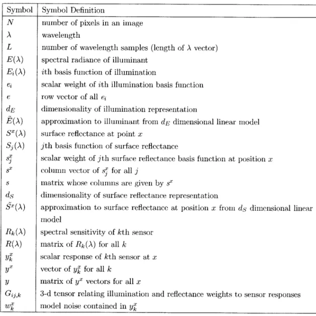
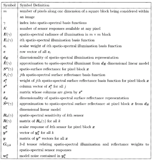
noise can be treated in the same manner as observation noise produced by the camera. An outline of all the symbol notation introduced above is given in Table 3.1.
While lower dimensional linear models allow for fewer parameters to be computed, they also produce larger amounts of model noise. Many researchers have examined the question of what dimensionality is required for these linear models in order to provide a "good" description of the data. For surfaces, it has been shown [30, 31, 35] that between 5 and 8 (depending on which data set was used) basis functions are needed to get a representation that accounts for greater that 99.5% or so of the variance of all surface reflectance spectra. Using as few as 3 basis functions can account for greater than 98% of the variance in these spectra. For natural illuminants, a 3 dimensional linear model accounts for 0.9997 of the variance according to [38]. Artificial lights, however, are not found to be very well fit by linear models since their spectra are not smooth.
Symbol Definition
N number of pixels in an image
A wavelength
L number of wavelength samples (length of A vector)
E(A) spectral radiance of illuminant
Ej (A) ith basis function of illumination
ej scalar weight of ith illumination basis function
e row vector of all eC
dE dimensionality of illumination representation
E(A) approximation to illuminant from dE dimensional linear model
SX(A) surface reflectance at point x
S (A) jth basis function of surface reflectance
six scalar weight of jth surface reflectance basis function at position x
sX, column vector of s, for all j
s matrix whose columns are given by sx
ds dimensionality of surface reflectance representation
Sx(A) approximation to surface reflectance at position x from ds dimensional linear
model
Rk(A) spectral sensitivity of kth sensor
R(A) matrix of Rk(A) for all k
yX scalar response of kth sensor at x
vector of yx for all k
y matrix of yx vectors for all x
Gij,k 3-d tensor relating illumination and reflectance weights to sensor responses
WX model noise contained in yx
Table 3.1: Symbol Notation for Standard Color Model I
3.2
Related Work
Color constancy has a long history in the image processing community, and the many existing approaches may be distinguished from one another not only by the differences between their solution strategies, but also by their formulation of the problem and the assumptions that they make. In this section we describe the most significant approaches found in the literature. Some of these methods (gray world, subspace, and Bayesian) model the image formation process explicitly and attempt to determine the full illumination and reflectance spectra at every point in the image. Others (gamut mapping, retinex, neural networks, color by correlation) attempt to find a single mapping from the input RGB image to the color corrected image without ever dealing explicitly with spectra. In this thesis we shall refer to these as inverse-optics and transformational approaches, respectively.
One approach to color constancy is to simply reformulate the problem so that it is not underconstrained. The subspace method does this by assuming the reflectance spectra can be adequately modeled using only two coefficients rather than three [32, 451. Given a trichromatic visual system and a three-dimensional illumination, an
N pixel image contains 3N data points and, under the subspace assumption, only
2N + 3 unknowns. In theory, we should be able to solve for all data points exactly.
This method fails in real images, however, because of the model noise (we will revisit the subspace method in Section 3.4.2).
The gray world algorithm [8] is an inverse-optics approach that assumes the aver-age reflectance of an imaver-age scene is equal to some known spectrum or, as an alternate formulation, that the average sensor response is equal to some constant value. In either case, the additional constraint allows for a straightforward solution. How-ever, because the gray world assumption is not very accurate one, solutions obtained through this method are not very accurate.
Retinex is a transformational algorithm that relies on the assumption that il-lumination causes only slowly varying color changes in an image, and attempts to
construct a color-corrected image by removing this effect [25, 24, 19]. The original
implementation of Retinex takes random walks across an image starting at randomly chosen pixels. The sensor responses at every pixel along a walk are scaled by the value of the starting pixel, and all ratios that are close to unity are set equal to 1. The out-put of the algorithm is the average of all scaled and thresholded values at each pixel. With the exception of the thresholding effect, the remaining computations amount to a scaling of the image by the brightest sensor value within the image. Other variants
of the Retinex algorithm have been presented which essentially differ from the original in that they scale the image by the mean (rather than the maximum) sensor value.
An alternate approach to color constancy is to take advantage of physical con-straints in the imaging system. Gamut mapping approaches [14, 13] utilize the prop-erty that the gamut of all possible RGB sensor responses under a given illumination can be represented by a convex hull. They model the effect of an illumination change as a linear transformation in RGB space, so that the convex hull of RGB values under one illuminant is related by a linear mapping to the convex hull of RGB values under another illumination. Thus, the illumination of a scene is estimated by finding the linear transformation that best maps the convex hull of the observed sensor responses to the known convex hull of all real world objects under white light.
The neural network approach [15, 16] examines the color constancy problem as if it were a classification problem. The image is transformed from the 3-d RGB color space into a 2-d RG-chromaticity space (in which the R and G channels are scaled by the sum of all three channels so that all values are between 0 and 1).
A discrete histogram of the RG-chromaticity values are fed into a neural network
which is trained to output the RG-chromaticity values of the illuminant. While this approach has produced some promising results, all of the assumptions it makes are implicit within the neural network and it is therefore difficult to understand exactly what it is doing.
The Bayesian approach to color constancy was introduced by Brainard and Free-man [6] as a means of incorporating both image statistics and physical constraints in an explicit manner. They began from the inverse-optics formulation of the problem and utilized truncated Gaussian distributions as priors on illumination and surface reflectance coefficients. In order to make estimation feasible, they performed estima-tion over the illuminaestima-tion coefficients using the maximum local mass technique, and solved for the surface reflectance coefficients at every iteration given the illuminant at that iteration. Nearly all of the other color constancy algorithms can be seen as a special instance of the Bayesian approach. Results using the general Bayesian formu-lation, however, have only been shown for synthetic images. Difficulties in modeling natural image statistics and implementation issues have prevented this approach from being used more extensively on real-world images.
Color by correlation is a transformational algorithm that borrows from the Bayesian approach. It uses a correlation matrix to estimate the scene illuminant given an observed image. This correlation matrix is equivalent to a discrete nonparametric likelihood function that describes how likely a set of surfaces are given a particular
illumination. Recent work more clearly reformulates the color by correlation method in a Bayesian framework and has been shown to achieve very good results [39]. This work explicitly models the imaging process as a linear transformation in RGB space with diagonal transformation matrix and incorporates a prior over the color-corrected image as well as a prior over illuminations that enforces physical realizability.
Many of the methods described above incorporate some form of information or statistic about the overall set of values in the reflectance image or the color-corrected image. None of them, however, incorporate any information about local image statis-tics of the form described in Section 1.3. We wish to examine if natural image statisstatis-tics that describe this local structure can assist in color constancy. To do so, we will build on the Bayesian color constancy algorithm of [6] as this method can most easily be extended to use additional statistical information.
3.3
Hyperspectral Data
To perform simulations, we use a hyperspectral data set of 28 natural scenes collected at Bristol University by Brelstaff, et. al. as described in [7]. Each of these images is
256 x 256 pixels in size and contains sensor responses in 31 spectral bands, ranging
from 400nm to 700nm in 10 nm intervals. Each scene also contains a Kodak graycard at a known location with a constant reflectance spectrum of known intensity. The scene illuminant is approximated as the spectrum recorded at the location of the graycard divided by its constant reflectance. The reflectance is then found by factoring out the illumination from the given hyperspectral signal (the reflectance images had to be thresholded to be less than or equal to one in some places). Our dataset therefore
consists of 256x256x28 reflectance spectra and 28 illumination spectra.
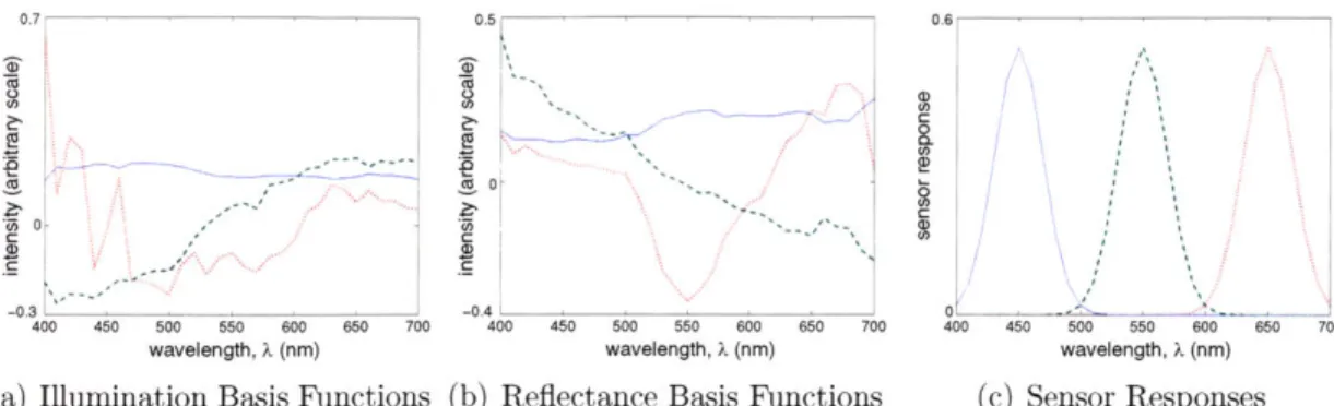
The first three illumination and reflectance basis functions, obtained by applying principal components analysis (PCA) to this data, are plotted in Figure 1(a) and
3-1(b), respectively (PCA is performed on all 28 illumination spectra and approximately
half of the available reflectance spectra). We assume, without loss of generality, a Gaussian model for sensor responses centered at 650nm (red), 550nm (green), and 450nm (blue) as shown in Figure 3-1(c). Sample images from the dataset, after being passed through these Gaussian sensors, are shown in Figure 3-2.
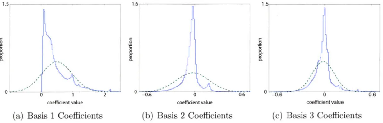
Normalized histograms of the coefficients corresponding to the first three re-flectance basis functions are shown in Figure 3-3. The best fitting Gaussian dis-tributions are shown as well. It can be seen that all of the coefficients associated with the first basis function are positive. This is as we would expect, since the first basis
0.7 0 -0.31 400 450 500 550 600 650 700 wavelength, X (nm) 0.5 0 -0.4 400 450 0 0 (0 a 500 550 600 650 700 wavelength, X (nm)
(a) Illumination Basis Functions (b) Reflectance Basis Functions
Figure 3-1: Linear models of reflectance and illumination spectral dataset, and assumed linear sensor responses.
400 450 500 550 600 650 700
wavelength, k (nm)
(c) Sensor Responses
obtained from the
hyper-Figure 3-2: Sample images from dataset of 28 hyperspectral images after being passed through the sensors of Figure 3-1(c). The hyperspectral images contain information from 31 spectral bands at each pixel, and the graycards in each of the images is used to find the true illumination of the scene.
IR - ;a -- M 103 -- ^ - - - -4-j
function is essentially constant (thus acting as a bias term), and all reflectance spec-tra must be nonnegative. The distributions for the next two coefficients are centered close to zero, and exhibit much greater kurtosis than the Gaussian approximation (as indicated by the "peakiness" of the histograms).
1.5 1.6 1.5
.0 0 0
0 1 2 0-0.6 0 0.6 006 0.6
coefficient value coefficient value coefficient value
(a) Basis 1 Coefficients (b) Basis 2 Coefficients (c) Basis 3 Coefficients
Figure 3-3: Histograms, obtained from the full hyperspectral dataset, of the coeffi-cients corresponding to the PCA reflectance basis functions shown in Figure 3-1(b). The best fit Gaussian (dashed) probability distributions are also shown.
3.4
Using Spatial Information: Spatio-Spectral
Ba-sis Functions
Although the existing Bayesian approach to color constancy allows a great deal of flexibility, it is limited to considering all image pixels to be independent of one another. In reality, the spatial configuration of image pixels are governed by physical properties of the world and are far from independent. By ignoring the spatial statistics of images, the existing approach does not utilize all of the information available.
The existing approach can be modified to incorporate the relationship between neighboring pixels by using linear models to describe the reflectance of groups of pixels, rather than individual pixels. Without loss of generality, we can group pixels into m x m blocks and use the same basic formulation as was developed in Section
3.1. In order to do so, it is necessary to convert blocks of pixels into vector format.
We do this by rasterizing the pixels within the block. The reflectance of a block of pixels is defined as a vector of length m2L consisting of the reflectance of each pixel
within the block stacked on top of each other in raster order. The same process is used to describe the sensor response of the block as a vector of length m2K and the
The basis functions used to model the reflectances of the blocks of pixels are now referred to as spatio-spectral reflectance basis functions, since they implicitly describe both the spectral and spatial (within an m x m block) characteristics of a block of pixels.
We shall denote a group of pixels by x, so that the illumination and reflectance of a block of pixels is given by:
m2L
E(y) - E (-y)e, (3.9)
m2 L
SX () Z S ()si, (3.10)
j=1
where Ej (-y) and S (-y) are the spatio-spectral illumination and reflectance basis func-tions, ej and si are the weights associated with these basis functions, E( ) is the illumination of all blocks in the image, and Sx(-y) is the reflectance of the block of pixels x. Note that the elements of the scene are now written as a function of 'Y rather than A. This is due to the fact that the spatio-spectral representation contains information about both the frequency and spatial characteristics of the scene, so it cannot be parameterized by the wavelength (A) alone. Approximating these models with fewer dimensions, we can define
dE
E(y) = E(-) e, (3.11)
ds
SXQ(b) =- Sj ()Si, (3.12)
j=1
where E(-y) is the approximate illumination of all blocks in an image, constructed using a dE dimensional model, and Sx(-y) is the approximated reflectance for the block x, constructed using a ds dimensional model.
We define an m x m block of pixels as having m2K sensor outputs, with K sensor
block diagonal matrix
R(A) 0 0
R(7) R(A) .. (3.13)
0 0 0 R(A)J
with m2 blocks along the diagonal, where
R(A) = [R 1(A) R2(A) ...
RK(A)]-We let Rk(7) refer to the kth column of the matrix R(y).
Following a derivation analogous to that presented in Section 2, we can write the sensor output in a bilinear form with noise as:
dE ds
y =
S
esGij,ksj + wT, (3.14)i=1 j=1
where y- is the sensor response of the block of pixels x, Gij,k is defined as
Gij,= Rk(-) Ej(-) Sj (y), (3.15)
and w' is the noise introduced from using a lower-dimensional linear model.
3.4.1 Characteristics of Spatio-Spectral Basis Functions Figure 3-4 plots the first 12 spatio-spectral reflectance basis functions when consider-ing a 2 x 2 pixel blocksize. These basis functions were extracted from our hyperspectral data using the calibration gray card in each image of the dataset, as described in Sec-tion 3.3. The correlaSec-tion between neighboring pixels in the 2 x 2 block is apparent when examining these basis functions. Discarding sign, it can be see that the first three spatio-spectral basis functions are essentially the same as the basis functions for the single pixel shown in Figure 3-1(b), repeated across all four pixels in the 2 x 2 block. That is, the first three basis functions exhibit virtually no spatial variation. To some extent, Figure 3-1(b) shows a separability between the spatial and spectral characteristics of the reflectance. Ruderman [41] has shown a similar result when examining images in terms of their L,M,and S cone responses.