Acceptable Reforms of Agri-environmental Policies
Philippe Bontems
University of Toulouse (INRA and IDEI)
Gilles Rotillon
University of Paris 10 Nanterre (THEMA)
Nadine Turpin
INRA Rennes and Cemagref Clermont Ferrand
Selected Paper prepared for presentation at the American Agricultural
Economics Association Annual Meeting, Providence, Rhode Island,
July 24-27, 2005
Copyright 2005 by Bontems, Turpin and Rotillon. All rights reserved. Readers may make
verbatim copies of this document for non-commercial purposes by any
Acceptable reforms of agri-environmental policies
Philippe Bontemsy Gilles Rotillonz Nadine TurpinxApril 2005 Preliminary draft.
Abstract
We consider a model of regulation for nonpoint source water pollution through non linear taxation/subsidization of agricultural production. Farmers are heterogenous along two dimensions, their ability to transform inputs into …nal production and the available area they possess. Asymmetric information and participation of farmers to the regulation scheme put constraints on the optimal policy that we characterize. We show that a positive relationship between size of land and ability may exacerbate adverse selection e¤ects. We then introduce acceptability constraints and show that the intervention under acceptability amounts to reallocate production towards ine¢ cient farmers who bene…t from the reform at the expense of e¢ cient producers. Last, we calibrate the model using datas on a french watershed (Don watershed). Simulations indicate that satisfying a high degree of acceptability does not entail high welfare losses compared to low degree of acceptability.
JEL: D82, Q19.
Key-words : Non Linear Taxation - Asymmetric Information - Non Point Source Pollution - Water Pollution.
We acknowledge …nancial support from EU through AgriBMPWater project (5th PCRD). Senior author-ship is not assigned. Corresponding author: Gilles Rotillon.
yUniversity of Toulouse (INRA, IDEI). zTHEMA, University of Paris-X Nanterre.
1
Introduction
The use of economic incentive instruments such as green taxes in environmental policy has become increasingly popular in many countries and in particular in Europe. However, new taxes are often unpopular in polluting sectors that usually prefer traditional command and control regulation. When designing a green tax scheme, the regulator has thus to take into account the potential losses imposed to the polluters when comparing with the pre-reform (or status quo) situation. In other words, the design of green reforms is subject to a political acceptability constraint.
On the one hand, the tax scheme can be designed such that no producer looses through a reimbursement rule using lump sum transfer. This means that any polluting …rm would enter voluntarily in the environmental regulation scheme given that there are no losses compared to the status quo situation. Such a highly acceptable policy comes usually at an ine¢ ciency cost: in order to be acceptable by everybody, the environmental regulation should not impose too much e¤ort. Otherwise, a high level of abatement would be too costly. On the other hand, the government might impose the term of regulation without fearing about losses imposed to polluters. In such a case, the strong commitment power of the government allows it to push forward a mandatory regulation. Of course, such a political power might be limited by laws protecting polluters’revenues by limited liability up to a given amount. The resulting policy would be highly e¢ cient from an environmental perspective but would gain very low political support in the polluting industry. (ex taxe CO2, rapport OCDE)
The concern about political support for reform is particularly deep in the agricultural sector in Europe. Rising concerns about environmental quality depressed by highly intensive agriculture have given birth to a series of reforms relating the level of subsidy to the environ-mental e¤ort of farmers. Up to now, those policies have largely relied on voluntary adoptions by farmers and have gained little success. Some have argued that o¤ered compensations were insu¢ cient to cover the compliance cost and that uncertainty about the durability of
envi-ronmental voluntary programs have undermined their success. A large rate of participation is obviously needed to attain environmental protection goals, so that ensuring this rate in a voluntarily way might be excessively costly. This situation raises the issue of how to regulate agricultural pollution abatement while sustaining a given level of political support.
In this paper, we consider water pollution caused by agricultural activities and we ana-lyze how to regulate farmers’ behavior while taking into account the pro…t potential losses induced by the reform. Of course, it is well known that regulating agricultural pollution is quite di¢ cult because of the non point source feature: individual emissions cannot be mea-sured and controlled easily (see Shortle and Horan (2001) for a survey). To overcome this di¢ culty, we consider the regulation of nonpoint source water pollution by an environmental agency through non linear taxation/subsidization of agricultural production and land. Those variables are more easily observable than individual emissions. The population of farmers we consider is heterogenous along two dimensions: their ability to transform inputs into …nal production and the available area they possess. Productive ability is assumed to be private information to the farmers while available area is an observable characteristic which may be part of the regulatory scheme. Hence, private information makes self-selection necessary. In addition, we assume that farmers’pro…ts are protected by limited liability such that the reform cannot yield negative pro…ts.
We introduce political acceptability as part of the constraints that the regulator has to take into account. Following Lewis et al. (1989), the regulator has to satisfy a given proportion of farmers through intervention and a farmer is satis…ed if he does not loose from regulation compared to the status quo situation.1 When this proportion is zero, the resulting policy is such that the political acceptability constraint is non binding and hence it can be labelled as a mandatory policy, which however does not allow the agency to impose negative pro…ts to farmers because of limited liability constraints. On the contrary, when this proportion is
1
The properties induced by the use of this criterion have been rarely studied in the economic literature. A recent exception is Demange and Geo¤ard (2002) who analyzed the physician regulation.
one, the policy is voluntary by its very nature as any farmer is ready to accept the reform. Bontems et al. (2004) analyze the mandatory case in details and show that asymmetric information yields to a larger range of less e¢ cient farmers that are induced to quit the sector and a lower production level for any type of farmers compared to what prevails when individual ability is perfectly known to the agency. Overall, the total level of pollution is reduced because …rst the less e¢ cient and most polluting farms are shut down and second because the remaining active farms are required to produce less intensively and therefore pollute less compared to the pre-reform situation.
This paper is devoted to the case where the proportion of farmers who have to be satis…ed is strictly positive. The identity of winners is endogenous and determined by the agency as part of the optimal policy. Two regulatory regimes are identi…ed. When the required level of acceptability is low, the regulatory pattern is similar to the mandatory one except that all farmers are now provided with a strictly positive level of pro…t which allows the agency to meet the acceptability constraint. When this level of acceptability is high, the regulatory pattern is quite di¤erent and entails pooling for a subset of farmers at the equilibrium, due to the presence of countervailing incentives. The regulatory regime depends on the observable farm area. We indicate the optimal rule of allocation of satis…ed farmers according to their characteristics. Importantly, an acceptable reform amounts to reallocate production towards less e¢ cient farmers who bene…t from the reform at the expense of more e¢ cient producers. In the last part of the paper, we calibrate the model using data from a French watershed (Don watershed) and we simulate the optimal policy under di¤erent scenarii concerning the weight of acceptability constraints from farmers. For this, we elaborate a speci…c method to classify farmers along a one dimensional type that represent their productive ability. We also use the results of a hydrological model calibrated on the watershed in order to estimate nitrogen emissions. Damages are estimated by computing the retreatment cost necessary to meet water quality standards actually enforced in Europe (upper limit on nitrogen water concentration). We show that, on our particular application case, satisfying a high degree of
acceptability does not entail high welfare losses compared to a low degree of acceptability. However, the environmental damages varies highly with the level of political support required. The paper is organized as follows. Section 2 is devoted to assumptions and notations and analysis of regulation under complete information. Regulation when self selection is necessary is analyzed in section 3 while section 4 is devoted to the empirical application to the Don watershed. Section 5 concludes. Most proofs are relegated into an appendix.
2
The model
2.1 The farmer’s behavior
We consider a farmer whose …nal output y (say milk) is produced using a quantity s of land devoted to feed crops and a polluting input such as fertilizers. Let us denote c(y; ) the production cost per unit of land. We introduce heterogeneity among farmers through parameter that belongs to the set = ; and that represents the farmer’s ability to transform feed crops into the production of milk. Parameter can be understood as a function of several on-farm characteristics (management skills, soil quality, genetic value of the herd...).
We assume that the cost of production c(:; ) is increasing convex in y. We also normalize the set of types by assuming that cost c is decreasing in . In addition, the marginal cost of producing milk is also decreasing with ability (cy < 0): In other words, a more e¢ cient farmer (higher type) is also associated with lower optimal rates of input use.2
Total land available for the production we consider is denoted by S which belongs to the set S = S; S . Land capacity S is distributed according to land density function h(S) with cumulative H(S). We also normalize the total land devoted to agriculture to unity. For each land capacity S, there is a continuum of farmers characterized by their ability, with mass unity. Farmers are distributed along this line segment according to ability density function f ( ; S) with cumulative function F ( ; S): We assume that f ( ; S) > 0 for every and S: Note
2
In addition, we make the following technical assumptions: cyy < 0, c y > 0. These assumptions will help us in obtaining optimal policies that e¤ectively separate the di¤erent farmers.
that we also assume that the set does not depend on S.3 However, this assumption does not presume that and S are independent. Moreover, the risk ratios 1 F ( ;S)f ( ;S) and F ( ;S)f ( ;S) are assumed to be strictly increasing in .4
Let us describe the private optimum of the pro…t-maximising farmer with ability and land capacity S, assuming there is no intervention by the environmental agency (status quo situation). It is given by solving the following program :
max
s;y (s; y; ) (py c(y; ))s
s.t. s S
where p is the (exogenous) product price. We assume that market and production conditions are such that all farms are active in the status quo situation. Hence the constraint s S is binding everywhere.5 We denote y ( ) as the optimal production level of type- farmer. Given our assumptions on c(:; :), it is easy to check that both the optimal production level y ( ) and the corresponding pro…t level ( ) are increasing in the farmer’s ability .
2.2 The Environmental Agency objective
Agricultural lands not only di¤er according to their productive e¢ ciency but also in the environmental impacts of production. We assume that pollution is represented by a pol-lution production function per hectare, denoted g(y; ), that estimates the emissions using simulation models, where g(:; :) is increasing with y and depends on . We do not impose assumptions on the sign of g that may vary: this is indeed the case on our empirical appli-cation. As a consequence, a more e¢ cient farmer may or may not pollutes less at the margin
3This assumption can be relaxed but at a much higher cost of complexity for the analysis. In that case, it is possible to diminish incentives costs because private information is partially veri…able by the regulator (see Green and La¤ont 1986).
4These regularity conditions are made in order to prevent the incidence of “pooling” in the optimal policy resulting from the probability function, that is policy in which the same allocation is selected for di¤erent values of .
5
Alternatively, we could have considered that the optimal cropped area s is interior, simply by adding a …xed cost k(s) for land in the pro…t function: (s; y; ) (py c(y; ))s k(s):This extension is straightforward and does not modify drastically the features of the optimal policy derived in the paper.
ceteris paribus. We denote E the total pollution level for the watershed: E = Z S S Z sg(y; )f ( ; S)d h(S)dS
The problem of the regulatory (utilitarian) agency is to maximize a social welfare function W, written as the sum of taxpayers surplus, the farmers total surplus and the environmental damage D. We assume that the social cost of pollution D(E) depends on total pollution emitted and is increasing, convex. Note that we do not include any consideration to the consumer surplus in the welfare function. As the regulation is implemented on a small watershed in our empirical application, we expect that any variation in the agricultural production given the regulation will have negligible impacts on total production sold on the market.
As emphasized in the introduction, both the land e¤ectively used and the level of pro-duction are assumed to be observable and veri…able by anybody. Suppose that the regulator requests the -type farmer with land capacity S to produce output y( ) using land s( ) S and o¤ers the monetary transfer t( ):6 The corresponding pro…t of the -type farmer can be written as follows:
( ) = (py( ) c(y( ); ))s( ) + t( ) (1)
Note that if the regulator requests s( ) to be strictly inferior to S then set-aside is part of the regulatory proposal for a -type farmer with land capacity S. In particular, the regulator may …nd optimal to shut down some farmers by assigning them s( ) = 0.
The regulatory’s objective can be expressed as
W Z S S Z [ ( ) (1+ )t( )]f ( ; S)d h(S)dS D Z S S Z s( )g(y( ); )f ( ; S)d h(S)dS !
where is the (positive) marginal cost of public funds. Eliminating the transfer t(:) and
6
using (1), we obtain a reduced formulation of the regulator’s objective function: W = Z S S Z [(1 + )(py( ) c(y( ); ))s( ) ( )]f ( ; S)d h(S)dS D Z S S Z s( )g(y( ); )f ( ; S)d h(S)dS !
Finding the optimal policy amounts to …nd the land allocation s(:); the production level y(:) and the net pro…t (:) (or equivalently the transfer t(:)) that are feasible in a sense to be precised below and that maximize the welfare function.
2.3 Incentive compatibility and acceptability constraints
Feasible allocations are …rst constrained by the information set of the regulator. Information asymmetry arises from the impossibility for the regulator to identify each farmer’s ability. Alternatively, one may assume that ability is observable but that institutional or political constraints prevent the regulator from perfectly discriminating farmers on that basis. Thus, a self-selecting policy remains the only option available to the regulatory agency. Following the Revelation Principle (Myerson, 1982) we can restrict our attention to the set of direct revelation mechanisms fs( ); y( ); t( )g 2 .
By choosing a particular contract among all o¤ered contracts, say a production level y(^), a forage area s(^) in exchange of a tax/subsidy t(^), a farmer implicitly announces to be of type ^. Hence, incentive compatibility requires to satisfy the following constraints:
( ) ( ; ^); 8 ; 8 ^ (IC)
where ( ; ^) = ps(^)y(^) s(^)c(y(^); ) + t(^) and ( ) ( ; ), which ensures that any farmer …nds optimal to reveal his true type.
The regulator’s problem is to design policies which are not only incentive compatible but also politically acceptable. Consequently, the regulator has to operate under the additional constraint that the policy has to be acceptable compared to the status quo policy, and can therefore be implemented and enforced. This allows the regulator to take into account the
regulatory history in the agricultural sector before formulating the reform. Following Lewis, and al. (1989), suppose that only the farmers who bene…t from the policy will support it, and that the probability that a farmer will support the policy is strictly positive if only if his pro…t after the reform is greater than before, i.e. ( ) ( ). More precisely, we denote ( ( ) ( )) this probability and we assume for simplicity that (:) = 1 whenever ( ) ( ) and 0 either: The political implementation of the policy requires that the following acceptability constraint should be taken into account:
Z S S
Z
( ( ) ( ))f ( ; S)d h(S)dS (AC)
which indicates that the probability that the policy is accepted must be superior to a (exoge-nous) level 2 (0; 1].7 In addition, we assume that any farmer is free to leave the agricultural sector following the reform. This implies that the pro…t obtained after the reform cannot be lower than the reservation pro…t. Assuming that the best outside option for any type of farmer yields a constant (not type dependant) pro…t, we normalize this reservation pro…t to 0 and we obtain the following individual rationality constraints:
( ) 0; 8 (IR)
In this setting, the regulator is thus able to enforce its policy as long as it does not entail any net loss for farmers and provided that a proportion of farmers gets after the reform at least the income earned before.
Finally, we impose that the optimal production level after the reform cannot be greater than the level under the status quo situation (8 ; S; y( ) y ( )). Hence we forbid any re-allocation of production across farmers such that some of them may be given incentives to produce more than their private optimum absent any regulation. First, we believe that this constitutes a reasonable property of the optimal policy as it should facilitate political support for the regulatory intervention given that all farmers have to make some e¤ort by reducing production. Second it helps us in deriving the optimal policy as will be clear below.
7
This way of modelling political constraints is also recently investigated by Demange and Geo¤ard (2002) in a model of physician regulation.
Given the various constraints faced by the regulator, the program to be solved is as follows:
max
s(:);y(:); (:)W s.t. (IC), (IR), (AC), s( ) S and y( ) y ( ) 8 ; S.
Obviously, it is clear that the addition of the acceptability constraint to the regulator’s maximisation program always induces a loss in welfare compared to the situation of a so-called mandatory policy which is obtained for the special case = 0. It remains important to ascertain the qualitative changes in the optimal regulatory policy when varies. Moreover, when = 1, it is also interesting to note that our model belongs to the class of adverse selection models with type-dependant participation constraints (Jullien (2000)).8 However, in the general case where 2 (0; 1), the type-dependant participation constraint only applies to an endogenous subset of types (the “winners” of the reform) which must be identi…ed as part of the optimal policy.
2.4 Regulation under complete information
Before analyzing the optimal self-selecting policy, we characterize in this section the optimal policy under complete information, ignoring incentive compatibility constraints (IC). The program to be solved is:
max
s(:);y(:); (:)W s.t. (IR), (AC), s( ) S and y( ) y ( ) 8 ; S.
Ignoring the constraint y( ) y ( ) for the moment, we di¤erentiate the objective w.r.t. y( ) and we obtain the following necessary conditions:
(1 + )(p cy(yP I( ); )) = D0 EP I gy((yP I( ); )) (2)
where P I denotes perfect information and EP I =RSSR sP I( )g(yP I( ); )f ( ; S)d h(S)dS. Equation (2) indicates that for an active farmer the optimal production level yP I( ) is deter-mined by equalizing social marginal bene…t and social marginal damage. Given the linearity
8
In this class of adverse selection models, countervailing incentives are generally part of the optimal policy because of the interaction between the incentive compatibility constraints and the type-dependant participation constraints. See also Lewis and Sappington (1989) and Maggi and Rodriguez-Cläre (1995) for earlier analysis on countervailing incentives.
of pro…t function with respect to the land input, the optimal production does not depend on the land capacity S. Moreover, it can be checked readily from equation (2) that the optimal regulation entails a decrease in production per hectare compared to the private optimum (i.e. yP I( ) < y ( ) for any ).
Then, di¤erentiating the objective w.r.t. s( ) we get: @W
@s( ) = ( )f ( ; S): where
( ) = (1 + )(pyP I( ) c(yP I( ); )) D0 EP I g(yP I( ); )
denotes the social net marginal surplus of land. We assume that ( ) is increasing and that ( ) > 0 otherwise all farmers should be shut down.9 It follows that when ( ) < 0 there exists a unique threshold type P I(S) such that for any S, whenever P I, the farmer is not allowed to produce (8S, sP I( ) = 0, 8 P I(S)). On the contrary, the more e¢ cient farmers produce using their total land capacity (8S, sP I( ) = S, 8 > P I(S)). Finally, when ( ) > 0, then all farmers are allowed to produce at the optimum involving complete information.
To complete the description of the optimal policy under perfect information, it remains to characterize the redistribution policy (through the transfer) inside the population. As the objective is decreasing in the rent ( ) left to any agent, it is clear that the regulator would like to bind all participation constraints at the optimum ( ( ) = 0, 8 ; 8S). Of course, such a policy is not politically acceptable as long as is strictly positive. In the limit case where all farmers must be compensated ( = 1), the regulator has to o¤er a compensation tP I( ) = ( ) ~P I( ) > 0 to any -type farmer (with land size S) where ( ) is the pro…t before the reform and ~P I( ) = (pyP I( ) c(yP I( ); )sP I( ) is the pro…t gross of transfer under the reform.
9Di¤erentiating ( )w.r.t. and using (2) leads to 0( ) = (1 + )c (yP I( ); ) D0 EP I g (yP I( ); ): ( )is increasing given that c < 0 and provided that g is negative or not too positive, which is guaranteed in our empirical application.
In intermediate cases when 0 < < 1, the identity of compensated farmers is determined by the shape of ( ) ~P I( ). Unfortunately, this results in very various situations depending on the model speci…cation. As we will see now, incomplete information puts more structure on the shape of the optimal pro…t and gives clearer predictions on the identity of compensated farmers.
3
Regulation under incomplete information
The regulator has now to solve the following program: max
s(:);y(:); (:)W s.t. (IC), (IR), (AC), s( ) S and y( ) y ( ) 8 ; S.
Standards arguments (see Guesnerie and La¤ont, 1984) indicate that incentive constraints can be replaced by the following set of constraints:
0( ) = c (y( ); )s( ) (IC1)
s0( )c (y( ); ) s( )c y(y( ); )y0( ) 0 (IC2)
Because the rate of growth of rents is positive ( 0( ) > 0), then participation constraints reduce to ( ) 0:
3.1 Preliminary analysis
Denote ya( ), sa( ), a( ) as the optimal second best allocation o¤ered to any type- farmer for a given land capacity S. For each land capacity S, we know that the set of farmers allowed to produce will be an interval a(S); . Now, let us examine the constraint (AC). At least for some S, the continuous functions a( ) and ( ) must clearly intersect or touch at least once, otherwise (AC) would be violated or it would not bind, which is suboptimal.
We will proceed in two steps. First, we characterize the optimal policy for a given class of surface S under the constraint that the proportion of farmers that gain from the reform is at least (S) which is given, i.e.
Z
Second, we determine the optimal pro…le for the proportions (S) under the constraint RS
S (S)h(S)dS = .
For that purpose, let us denote WS the welfare function (partially) restricted to the class of surface S, assuming that the policy for any S0 6= S is …xed to the optimal level (i.e. ya( ), sa( )):
WS = Z
[(1 + )s( )(py( ) c(y( ); ) ( )] f ( ; S)d D(E) where the total level of pollution E is rewritten as follows:
E = Z S S Z sa( )g(ya( ); )f ( ; S0)d h(S0)dS0+ Z s( )g(y( ); )f ( ; S)d h(S) + Z S S Z sa( )g(ya( ); )f ( ; S0)d h(S0)dS0:
Actually, the following lemma indicates that, for a given S, the function a( ) intersects once ( ) from above at a point (S) if (S) is interior.
Lemma 1 For a given S, if (S) 2 (0; 1), then
(i) a( ) intersects ( ) once and from above at a point (S) 2 , (ii) (S) satis…es (S) = F ( (S); S).
Proof. see appendix A.
As shown by Lemma 1, it is important to note that incentive compatibility constraints and the constraint 8 ; S; y( ) y ( ) together imply that the set of farmers who bene…t from the reform is composed of the less e¢ cient producers whether they are active or not. Furthermore, the relative position of the threshold type a(S) and the intersection point (S) is crucial for the pattern of the optimal policy. First the function ( ) intersects a( ) on the ‡at part of a( ). This case occurs when (S) is "small" and we have a(S) > (S). Then necessarily ( (S)) = a( a(S)). On the contrary, the function ( ) intersects a( ) on the increasing part of a( ): This occurs when the proportion (S) is "large" and we have
3.2 The case when the proportion (S) is "small"
By a continuity argument, when (S) is "small", we expect that the optimal policy looks like the optimal mandatory one (i.e. for (S) = 0). This is shown in the following proposition.
Proposition 1 For any S such that (S) is "small", the set of farmers that are allowed to produce using their land capacity S is a(S); with a(S) > (S) and the optimal level of production for any type ( ; S) farmer is given by:
p cy(ya( ); ) = 1 1 + D 0(Ea) g y(ya( ); ) 1 + c y(y a( ); )1 F ( ; S) f ( ; S) where the total pollution level is
Ea= Z S S Z a(S)Sg(y a( ); )f ( ; S)d h(S)dS
Moreover, for any such that < a(S), production is not allowed (sa( ) = 0) and a( ) = a( a(S)) = ( (S)).
Proof. See appendix B.
As indicated by proposition 1, when (S) is "small", the optimal policy is similar to the mandatory one (i.e. when (S) is nil), except that the production levels and the range of excluded farmers are modi…ed because of the global pollution level Ea which is a priori dif-ferent. In particular, a positive distortion is added to the marginal damage when determining the optimal level of production for active farmers. Also, the minimum level of pro…t is now higher and equal to ( (S)) > 0 in order to ful…ll the acceptability constraint.
Finally, it is obvious that if the optimal repartition of the weights (S) across the classes of surface is such that (S) is "small" everywhere, then the optimal policy is totally identical to the mandatory one, except for the basic level of pro…t given to all farmers. Formally, we would then have Ea= E and (ya( ); sa( ); a(S)) = (y ( ); s ( ); (S)) for every S. However, the total welfare level is lower (and decreasing in (S)) compared to the mandatory one because of the social cost of giving a strictly positive minimum pro…t to every farmer. To sum up, in
that particular case, the introduction of the acceptability constraint only implies to translate upwards the minimum pro…t level for all farmers and does not change anything else to the optimal policy nor to the optimal level of pollution.
3.3 The case when the proportion (S) is "large"
We now turn to the opposite case where a(S) < (S) which occurs when (S) is "large". The optimal policy in that case is described in the following proposition.
Proposition 2 For any S, when (S) is "large", the set of farmers that are allowed to produce using their land capacity S is an interval a(S); with a(S) < (S) and the optimal level of production for any type ( ; S) farmer is continuous and de…ned by:
p cy(ya( ); ) = 1 1 + D 0(Ea) g y(ya( ); ) + 1 + c y(y a( ); )F ( ; S) f ( ; S); 8 2 [ a(S); 1(S)) , ya( ) = y(S); 8 2 [ 1(S); 2(S)] , p cy(ya( ); ) = 1 1 + D 0(Ea) g y(ya( ); ) 1 + c y(y a( ); )1 F ( ; S) f ( ; S) ; 8 2 2(S); , where the total pollution level is
Ea= Z S S Z a(S)Sg(y a( ); )f ( ; S)d h(S)dS
and where ya( ) denotes the quantities that maximizes WS and with y(S) maximizing expected welfare over [ 1(S); 2(S)] with a(S) 1(S) (S) 2(S) .. Moreover, for any such that < a(S), production is not allowed and a( ) = a( a(S)) > 0.
Proof. See appendix C.
As indicated in the proposition, the output pro…le is generally not e¢ cient. Indeed, holding the total level of pollution constant, we …nd that ine¢ ciently high levels of production are induced for low ability types while ine¢ ciently low levels of production are induced for highly productive farmers. The intuition is as follows. We knows that the acceptability constraint imposes that a( (S)) = ( (S)). For all types such that > (S), the farmer’s pro…t increases with its type at the rate of Sc > 0. The agency will thus tend to induce
lower output on this range in order to limit the rate of growth of informational rents. On the contrary, for < (S), the farmer’s pro…t decreases with its type at the rate of Sc < 0 and consequently, the agency tends to limit rents by inducing high levels of output. The pooling interval on [ 1(S); 2(S)], where all types of farmers are required to produce at the same constant level y(S) appears because around (S) the two tendencies exhibited above would require that output would decrease with ability which contradicts incentive compatibility (IC2). Thus, the agency has to induce the same level of production y(S) in the interval [ 1(S); 2(S)] around (S). Also the farmers in this range receive the same transfer level.
To sum up, the optimal policy involves an intermediary range of types producing the same level of production which maximize expected welfare while the farmers with lower ability are required to overproduce and the farmers with higher ability are required to underproduce. Compared to the situation where acceptability is not required (mandatory policy), it is clear that political participation induces the agency to reorganize production in a way that bene…t to the farmers with low ability. This is because essentially the revenue under status quo increases more rapidly than the revenue after intervention. Indeed for an active farmer, under the status quo we have 0( ) = Sc (y ( ); ) and incentive compatibility requires that 0( ) = Sc (y( ); ): Moreover, we have assumed that y( ) y ( ) and c is decreasing with y. Hence the revenue is more equally distributed in the population, so that the low-types farmers bene…t at the expense of high-low-types farmers. Subsidies given to the low-low-types farmers in order to induce them to leave the sector are …nanced through implicit taxation of high-types farmers. However, in our model, it is clear that the total level of pollution always decreases after intervention. Indeed, given that for any active farmer we have y( ) y ( ) and that the range of active farmers is smaller after regulation, total pollution is lower.
3.4 The optimal allocation of proportions (S)
In this subsection, we indicate the rule that determines the optimal allocation of proportions (S) across the surface classes. The regulator seeks to solve the following maximization
program: max (:) W = Z S S W Sh(S)dS s.t. WS = Z
[(1 + )sa( )(pya( ) c(ya( ); ) a( ) D(Ea)] f ( ; S)d
= Z S
S
(S)h(S)dS
We introduce a state variable (S) de…ned by _ (S) = (S)h(S) with the conditions (S) = 0 and (S) = . Let (S) denote the associated co-state variable. The lagrangian can be written as follows: L = Z S S W Sh(S)dS + Z S S (S) [ (S)h(S) _ (S)] dS = Z S S W S+ (S) (S) h(S)dS + Z S S _ (S) (S)dS (S) (S) + (S) (S)
and pointwise maximization leads to the following necessary conditions (for an interior opti-mum): @L @ = _ (S) = 0 ) (S) = 8S @L @ (S) = dWS d (S)+ = 0
Using the envelop theorem, it is easy to prove that dWS d (S) = 0( (S)) + Sc (y; (S)) @ (S) @ (S) = S c (y ( (S)); (S)) c (y(S); (S)) f ( (S); S) < 0:
Thus the marginal impact of (S) on expected welfare which is negative should be equalized across the di¤erent classes of surface.
4
Empirical application to the Don watershed
For this application, we used the same set of data from dairy farms collected for year 2000 on the Don watershed (Loire Atlantique, France) by Bontems et al. (2004). We shall summarize
here the main features of this empirical work.10 First, the critical issue in the application is to de…ne a unidimensional measure called “ability”( ) which allows to reduce the dimensionality of the set of acute parameters. Second, we have to estimate the density functions h(S) and f ( ; S) describing the population of farmers. Last, production cost, pollution and damage cost functions are estimated.
4.1 Determination of parameters
The parameter represents the ability for a given farmer to transform his forage area into dairy production. Its determination proceeds in two steps. Firstly, some experts in local extension services built a relative (one-dimensional) classi…cation of the surveyed farms, using observed variables such as the amount of dry matter produced by grasslands, the amount of milk produced per cow, the balance in forage feed between proteins and energy and the amount of required concentrates. Secondly these variables have been combined to recover the classi…cation proposed by the experts, and hence to determine a function which de…nes the one-dimensional parameter . A farmer who manages to obtain high grass yields, who breeds high productive cows, who gives them good quality forages and who needs low rates of concentrates to produce milk is considered to possess a good ability to transform his forage crops into milk, and thus his -parameter is high.
The distributions h(S) and f ( ; S) have been estimated using a discrete approximation of Beta density functions. Hence, farms are classi…ed into ten di¤erent classes of surface while ability falls into hundred di¤erent classes for each S.
Following Yiridoe et al. (1997), the amount x(y; ) of N fertilizer used is expressed as a quadratic function of production y. The cost function c(y; ) is then written as follows :
c(y; ) = w#( )x(y; ) + !( )y + %
where w is the inorganic N price, #( ) is a proportionality factor of fertilizers in forage operation costs, and !( )y + % represents the cost related to breeding operations.
Moreover, individual emissions have been estimated using a local hydrologic model (Turpin et al., 2001) from data collected on the surveyed farms and other data concerning soils, hy-drology and local climate on the Don watershed. Type-dependent emissions have been de-termined from these estimations, using a quadratic function and a constrained maximum likelihood method (Gouriéroux and Montfort, 1995). Finally, the cost of social damage is valued as being the cost of water treatment for transforming brut water into drinking water (Falala, 2002).
4.2 Analysis (to be completed)
Instead of exploiting the …rst order conditions exhibited in the theoretical part of this paper, the optimal policies for the mandatory and the political regulation cases have been more easily determined by solving the regulator maximisation program directly. For this purpose we used Gams software (Brooke et al., 1998) and Conopt optimisation procedure (Drud, 1994).
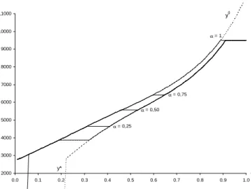
We will present successively the in‡uence of the required proportion of winners on production levels, after tax pro…ts and welfare. Figure 1 depicts optimal production levels for di¤erent scenarios concerning . The depicted situations correspond to Proposition 2 where is "large". As described in proposition 2, pattern of yaincludes two increasing parts and three pooling zones where all types are o¤ered the same contract. The …rst pooling zone corresponds to the set of excluded farmers which are the less productive ones (low ). In our application, the range of excluded farmers do not vary highly with . Then, for all active farmers, the regulatory intervention implies a decrease in production whatever the type and land capacity, except for a limited range where the constraint ya( ) y ( ) is binding. For the lower active types, the gap between the status quo and the optimal production levels is quite small.
The second pooling phenomenon appears because of the con‡ict between the acceptability (AC) and incentive (IC) constraints. Starting from this pooling zone towards the highest type,
the reform amounts to implement a larger decrease in production than before the pooling zone. The last pooling zone appears for the higher types of farmers and is due to the binding of second order conditions (IC2).
To sum up, we have imposed that every farmer must reduce his production level per hectare (ya( ) y ( )) under the reform. We have shown that on our empirical application an acceptable reform of agri-environmental policy implies to ask more e¤ort in terms of production reduction to high types compared to low ones, whatever the land capacity and the required acceptability level.
Figure 2 depicts pro…t patterns for a low value of (S) corresponding to proposition 2 and for a high value of (S) corresponding to proposition 3. For low values of (S), the simulated threshold value (S) is lower than a(S), which means that some inactive farmers loose money and this is true also for all active farmers. For high values of (S), a(S) becomes lower than (S). Consequently some active farmers now bene…t from the reform. When (S) is high, the loss of money imposed to the e¢ cient farmers ( a ) is lower than for smaller values of (S).
Moreover the ine¢ cient farmers receive a net subsidy while e¢ cient farmers are taxed : the e¢ cient farmers bear the cost of the reform.
Figure ? indicates that the optimal proportion (S) (weighted by the density h(S)) is increasing in for any class S. To compare di¤erent cases depending on the proportion of farmers who bene…t from the regulation we use indicators, constructed as a relative variation between the status quo and the regulated situations. We denote P( ) the relative variation of total pro…t:
P( ) = RS S R a ( )f ( ; S)d h(S)dS RSSR ( )f ( ; S)d h(S)dS RS S R ( )f ( ; S)d h(S)dS
And so are de…ned V( ), M( ), D( ), the relative variation of welfare, milk production and damage.
y0 α = 0,50 α = 0,75 α = 1 α = 0,25 2000 3000 4000 5000 6000 7000 8000 9000 10000 11000 0.0 0.1 0.2 0.3 0.4 0.5 0.6 0.7 0.8 0.9 1.0 θ y*
Figure 1: Optimal production levels for laissez-faire situation (y ) and di¤erent values of .
π0 α = 0.11 πa α = 0.06 5 10 15 20 25 30 35 40 45 50 55 0.00 0.05 0.10 0.15 0.20 0.25 0.30 0.35 θ π(1000 euros)
farmers who benefit from the regulation whenα = 0.11
farmers who benefit from the regulation whenα = 0.06
θ
π∗
Figure 2: Farmers pro…t as a function of -type for several cases : laissez-faire situation ( ), mandatory regulation ( ), low and high values of ( a).
of , we have the …rst regime for all S and proposition 2 applies, with ya( ) = y ( ) which is independent of . Thus M( ) and D( ) are constant : introducing acceptability constraints does not change the optimal policy compared to the mandatory case, except for the basic level of pro…t given to all farmers. This explains the decreasing level of pro…t loss (P( ) is increasing with respect to ). The farmers pay in expectation a tax to the regulator. As a consequence, the social welfare function is decreasing with respect to .
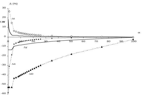
For values of higher than ?, Proposition 3 applies for some S and a(S) is strictly positive. Note that for the application, the monetary value of damage is rather low11 when compared with farms pro…t and tax paid by the farmers (Figure 3 depicts variations in percentage of the status quo level). The evolution of the welfare is mostly drawn by the variation of pro…t and transfer.
When exceeds, then all classes of surfaces fall under Proposition 3. Introducing ac-ceptability constraints when the proportion of farmers who bene…t from the regulation is growing lead to a decrease of social welfare with .
When is su¢ ciently high, the status quo situation is prefered by the regulator to inter-vention (V( ) becomes non positive). Except for the lower levels of , welfare gain compared to the status quo does not vary much with the level of acceptability.
5
Conclusion
We have considered a model of regulation for nonpoint source water pollution through non linear taxation/subsidization of agricultural production. Farmers are heterogenous along two dimensions, their ability to transform inputs into …nal production and the available area they possess. Asymmetric information and participation of farmers to the regulation scheme put constraints on the optimal policy that we characterize. We have shown that a positive relationship between size of land and ability may exacerbate adverse selection e¤ects. By introducing acceptability constraints we show that the intervention under acceptability
∆π ∆t ∆D ∆y ∆W -60 -50 -40 -30 -20 -10 0 10 20 30 0 10 20 30 40 50 60 70 80 90 100 ∆ (%) α
Figure 3: Relative variation with respect to of damage ( D), farmers’ pro…t ( ), milk production ( y), transfert from farmers to the regulatory agency ( t) and social welfare ( W). The mandatory regulation is not depicted here.
amounts to reallocate production towards ine¢ cient farmers who bene…t from the reform at the expense of e¢ cient producers. Last, we have calibrated the model using datas on a french watershed (Don watershed). Simulations indicate that satisfying a high degree of acceptability does not entail high welfare losses compared to low degree of acceptability.
References
[1] Babcock B.A. et al. (1997), “Targeting Tools for the Purchase of Environmental Ameni-ties”, Land Economics, 73, 325-339.
[2] Brooke A., Kendrick D., Meeraus A. and Raman R. (1998), GAMS a user’s guide, GAMS Development Corporation, Washington, 262 p.
[3] Cabe R. and Herriges J.A. (1992), “The regulation of non-point source pollution un-der imperfect and asymetric information”, Journal of Environmental Economics and Management, 22:134-146.
[4] Demange G. and P.Y. Geo¤ard (2002), “Reforming incentive schemes under political constraints: The physician agency”, mimeo, Delta, Paris.
[5] Drud A.S. (1994), “CONOPT - a large scale GRG code", ORSA Journal on computing, 6:207-216.
[6] Falala J., Lefèvre J., Mérillon Y. and Davy T., (2002), “Test de méthode d’analyse économique pour la mise en oeuvre de la directive cadre sur l’eau”, in "Lille III : From economic enigma to operational reality - Implementing the economic elements of the Water Framework Directive" (A. d. l. E. S. Normandie, Ed.), Lille,13p.
[7] Fleming R. A. and Adams R. M. (1997), “The importance of site-speci…c information in the design of policies to control pollution”, Journal of Environmental Economics and Management, 33, 347-358.
[8] Gouriéroux C. and Montfort A., (1995), Statistics and Econometrics models, Cambridge University Press, 562 p.
[9] Green J. and J.J. La¤ont (1986), “Partially veri…able information and mechanism de-sign”, Review of Economic Studies, 103:447-456.
[10] Gri¢ n R.C. and Bromley D.W. (1982), “Agricultural run-o¤ as a nonpoint externality : a theoretical development”, American Journal of Agricultural Economics, 64:547-542. [11] Guesnerie R. and JJ. La¤ont (1984) “A complete solution to a class of principal-agent problems with an application to the control of a self-managed …rm”, Journal of Public Economics, 25, 329-369.
[12] Helfand G.E. and House B.W. (1995), “Regulating nonpoint source pollution under heterogeneous condition”, American Journal of Agricultural Economics, 77, 1024-1032. [13] Holmstrom B. (1982), “Moral Hazard in Teams”, Bell Journal of Economics, 13:324-340. [14] Holtermann S. (1976), “Alternative Taxsystems to correct externalities and the e¢
-ciency of paying compensation”, Economica, 46:1-6.
[15] Horan R.D., Abler D.G., Shortle J.S. and Carmichael J. (2002a), “Cost-e¤ective point-nonpoint trading: An application to the Susquehanna River Basin”, Journal of the American Water Resources Association, 38, 467-477.
[16] Horan R.D., Shortle J.S. et Abler D.G. (1998), “Ambient Taxes When Polluters Have Multiple Choices”, Journal of Environmental Economics and Management, 36:186-199. [17] Horan R.D., Shortle J.S. et Abler D.G., (2002b), “Ambient Taxes Under m-Dimensional Choice Sets, Heterogeneous Expectations, and Risk-Aversion”, Environmental and Re-source Economics, 21:189-202.
[18] Jullien B. (2000), “Participation constraints in adverse selection models”, Journal of Economic Theory, 93:1-47.
[19] Larson D.M., Helfand G.E. et House B.W., (1996), “Second-best tax policies to reduce nonpoint source pollution”, American Journal of Agricultural Economics, 78:1108-1117.
[20] Lewis T.R., Feenstra R. and R. Ware (1989) “Eliminating price supports”, Journal of Public Economics, 40, 159-185.
[21] Lewis T.R. and D. Sappington (1989), “Countervailing incentives in agency problems”, Journal of Economic Theory, 49:294-313.
[22] Segerson K., (1988), “Uncertainty and incentives for nonpoint pollution control”, Journal of Environmental Economics and Management, 15:87-98.
[23] Shortle J.S. et Dunn J.W., (1986), “The relative e¢ ciency of agricultural source water pollution control policies”, American Journal of Agricultural Economics, August :668-677.
[24] Shortle J.S., Horan R.D. and D.A. Abler (1998) “Research issues in nonpoint pollution control”, Environmental and Resource Economics, 11, 571-585.
[25] Shortle J.S. and Horan R.D. (2001), “The economics of nonpoint pollution control”, Journal of Economic Surveys, 15, 255-289.
[26] Smith R.B.W. and Tomasi T.D., (1995), “Transaction Costs and Agricultural Nonpoint-Source Water Pollution Control Policies”, Journal of Agricultural and Resource Eco-nomics, 20:277-290.
[27] Turpin N., Granlund K., Bioteau T., Rekolainen S., Bordenave P. and Birgand F., (2001), “Testing of the Harp guidelines #6 and #9, last report : results”, Cemagref and FEI, Rennes,43 p.
[28] Weersink A. and al., (1998), “Economic Instruments and Environmental Policy in Agri-culture”, Canadian Public Policy, 24:309-327.
[29] Weinberg M. and King C.L., (1996), “Uncoordinated agricultural and environmental policy making : an application to irrigated agriculture in the West”, American Journal of Agricultural Economics, 78:65-78.
[30] Wu J.J., Teague M.L., Mapp H.P. and Bernardo D.J., (1995), “An empirical analysis of the relative e¢ ciency of policy instruments to reduce nitrate water pollution in the US southern high plains”, Canadian Journal of Agricultural Economics, 43:403-420.
[31] Wu J. and B.A. Babcock (1996) “Contract design for the purchase of environmental goods from agriculture”, American Journal of Agricultural Economics, 78, 935-945.
[32] Wu J. and B.A. Babcock (1999) “The relative e¢ ciency of voluntary vs mandatory environmental regulations”, Journal of Environmental Economics and Management, 38, 158-175.
[33] Yiridoe E.K., Voroney R.P. and Weersink A., (1997), “Impact of alternative farm man-agement practices on nitrogen pollution of groundwater: Evaluation and application of CENTURY model”, Journal of Environmental Quality, 26:1255-1263.
Appendix
A
Proof of lemma 1
Proof of part (i): Using the envelop theorem, we get before any regulation 0( ) = Sc (y ( ); ). As c y < 0 and ya( ) y ( ), we have:
c (ya( ); ) c (y ( ); )
But we have also sa( ) S; so using equation (??) we obtain:
0 a0( ) 0( )
If (S) > 0, then a( ) intersects ( ) once and from above, either on the ‡at part or on the increasing part of a( ).
Proof of part (ii): given (i), for the constraintR ( ( ) ( ))f ( ; S)d (S) to be binding at the optimum, (S) must satisfy (S) =R (S)f ( ; S)d = F ( (S); S).
B
Proof of proposition 1
Assume that 0 < (S) < a(S). Then, integrating (IC1), we get:
( ) = (
( (S)) for a(S)
( (S)) R a(S)c (y(u); u)s(u)du for > a(S)
: (3)
Using (3), we rewrite the objective WS as follows:
WS = Z a(S) [(1 + )s( )(py( ) c(y( ); )] f ( ; S)d Z a(S)h ( (S))if ( ; S)d Z a(S) " ( (S)) Z a(S)c (y(u); u)s(u)du # f ( ; S)d D(E)
Integrating by parts, we obtain:
WS =
Z
a(S)
(1 + )s( )(py( ) c(y( ); )) + s( )c (y( ); )1 F ( ; S)
f ( ; S) f ( ; S)d (4) ( (S))
Z
It remains to maximize WS w.r.t. s(:) and y(:). It is then clear that the optimal allocation (s(:); y(:)) follows the same rule as the one under a mandatory policy.
We now check that equation IC2 is satis…ed. For any type-( ; S) farmer who is allowed to produce, equation IC2 can be written as:
Sc y(y( ); )y0( ) 0
Derivating the …rst-order condition for y with respect to , and dropping any argument, we get: (1 + )(cyyy0+ c y) D0(E)gyyy0 D0(E)g y + 1 F f (c yyy 0+ c y) + c y d d 1 F f = 0
This equation can be written as:
y0 =
(1 + )c y+ D0(E)g y 1 Ff c y c ydd 1 Ff (1 + )cyy D0(E)gyy+ 1 Ff c yy
We have already made the following technical assumptions: c y < 0; c yy < 0; c y > 0 and d
d 1 F
f < 0. Thus, if in addition g y < 0 and gyy > 0, then we have y0( ) > 0, 8 and the second order conditions are ful…lled.
C
Proof of proposition 2
Given Lemma 1, we can integrate (IC1), and we get: ( ) =
(
( (S)) +R (S)c (y(u); u)s(u)du for (S)
( (S)) R (S)c (y(u); u)s(u)du for > (S) (5)
Using the de…nition of pro…ts given by (5), we get for WS: WS= Z [(1 + )s( )(py( ) c(y( ); )] f ( ; S)d Z (S)" ( (S)) + Z (S) c (y(u); u)s(u)du # f ( ; S)d Z (S) " ( (S)) Z (S) c (y(u); u)s(u)du # f ( ; S)d D(E)
Integrating WS by parts, we get : WS = Z h(1 + )s( )(py( ) c(y( ); )) ( (S))if ( ; S)d (6) Z (S) s( )c (y( ); )F ( ; S) f ( ; S) f ( ; S)d + Z (S) s( )c (y( ); )1 F ( ; S) f ( ; S) f ( ; S)d D (E)
Before derivating (6), note that the expression of the derivatives will depend on whether is greater or lower than (S).
C.1 Analysis for < (S)
For < (S), derivating (6) with respect to y( ), we obtain the following …rst-order condition for an (interior) optimum:
@WS @y( ) = 0 ) (1 + ) [p cy(y a( ); )] g y(ya( ); )D0(Ea) cy (ya( ); ) F ( ; S) f ( ; S) = 0 (7) Similarly, with respect to s(:), we obtain the following expression for the social marginal surplus of land : @WS @s( ) = (1+ ) [py a( ) c(ya( ); )] f ( ; S) c (ya( ); )F ( ; S) g(ya( ); )D0(Ea) f ( ; S) Note that, sign(@WS=@s( )) = sign(B( )) where B( ) = (1 + ) [pya( ) c(ya( ); )] c (ya( ); )F ( ; S) f ( ; S) D 0(Ea)g(ya( ); ) (8)
Using (7) and dropping any argument, we get from (8) :
B0= (1 + )c c F f c d d F f D 0(Ea)g :
Note that when c is small with respect to the other terms, B0( ) > 0. Assuming B( ) < 0 and B( ) > 0, there exists a unique threshold type a(S) such that for every < a(S),
@WS=@s( ) < 0 and consequently sa( ) = 0 so that all su¢ ciently ine¢ cient farmers are shut down. Moreover, for any > a(S); @WS=@s( ) > 0 and consequently sa( ) = S. The threshold type separating active from inactive farmers is given by:
(1 + )(pya( a(S)) c(ya( a(S)); a(S)))f ( a(S); S)
D0(Ea) g(ya( a(S)); a(S))f ( a(S); S) = c (ya( a(S)); a(S))F ( a(S); S)
This equation means that the regulator equalizes the marginal surplus (net of damage) of keeping active the type- a(S) farmers with the corresponding incentive cost for all smaller type farmers (in proportion F ( a(S); S)).
C.2 Analysis for > (S)
For > (S), derivating (6) w.r.t y( ) yields to:
(1 + )(p cy(ya( ); ) = gy(ya( ); )D0(Ea) cy (ya( ); )
1 F ( ; S)
f ( ; S) (9)
Once again, the optimal production level follows the same rule as for the optimal manda-tory policy and for the optimal policy when (S) is "small".
C.3 Pooling around (S)
From (7) and (9), it is clear that ya( ) decreases discontinuously at = (S) (that is,
lim ! (S) ya( ) > lim
! (S)+ya( )). Thus, it is not possible to implement ya( ) without
violating incentive compatibility constraints (more precisely (??)). The optimal policy in-volves pooling with ya( ) = y(S) in a neighborhood [ 1(S); 2(S)] around (S) (Lewis and Sappington, 1989).
It remains to determine 1(S); 2(S) and y(S) . First, it is easy to show that ya( ) is continuous (see Lewis and Sappington (1989)). Then, rewriting the pro…t function for any
-type farmer, we get:
a( ) = 8 < :
( (S)) +R 1(S)c (ya(u); u)sa(u)du +R (S)
1(S)c (y(S); u)s a(u)du pour (S) ( (S)) R 2(S) (S) c (y(S); u)s a(u)du R 2(S)c (y
Denote AW (s( ); y( ); ) = (1 + )s( )(py( ) c(y( ); ) ( ) D(E): Then WS = R
[AW (sa( ); ya( ); )] f ( ; S)d : Di¤erentiating WS with respect to y(S), we get: dWS dy(S) = Z 2(S) 1(S) @AW (sa( ); y(S); ) @y f ( ; S)d = 0: