DTA2012 Symposium: Combining Disaggregate
Route Choice Estimation with Aggregate
Calibration of a Dynamic Traffic Assignment Model
The MIT Faculty has made this article openly available. Please share
how this access benefits you. Your story matters.
Citation
Ben-Akiva, Moshe, Song Gao, Lu Lu, and Yang Wen. "DTA2012
Symposium: Combining Disaggregate Route Choice Estimation with
Aggregate Calibration of a Dynamic Traffic Assignment Model."
Networks and Spatial Economics 15:3 (September 2015), pp
559-581.
As Published
http://dx.doi.org/10.1007/s11067-014-9232-z
Publisher
Springer Science+Business Media
Version
Author's final manuscript
Citable link
http://hdl.handle.net/1721.1/103140
Terms of Use
Creative Commons Attribution-Noncommercial-Share Alike
DTA2012 Symposium: Combining Disaggregate
Route Choice Estimation with Aggregate
Calibration of a Dynamic Traffic Assignment
Model
Moshe Ben-Akiva∗ Song Gao† Lu Lu‡ Yang Wen§ March 8, 2014
Abstract
Dynamic Traffic Assignment (DTA) models are important decision sup-port tools for transsup-portation planning and real-time traffic management. One of the biggest obstacles of applying DTA in large-scale networks is the cal-ibration of model parameters, which is essential for the realistic replication of the traffic condition. This paper proposes a methodology for the simul-taneous demand-supply DTA calibration based on both aggregate measure-ments and disaggregate route choice observations to improve the calibration accuracy. The calibration problem is formulated as a bi-level constrained op-timization problem and an iterative solution algorithm is proposed. A case study in a highly congested urban area of Beijing using DynaMIT-P is con-ducted and the combined calibration method improves the fits to surveillance data compared to the calibration based on aggregate measurements only.
∗
Edmund K. Turner Professor of Civil and Environmental Engineering, Massachusetts Institute of Technology, Room 1-181, 77 Massachusetts Avenue, Cambridge, MA 02139. Tel: +1 617-253-5324. Email: [email protected]
†
Associate Professor, Department of Civil and Environmental Engineering, University of Mas-sachusetts, 214C Marston Hall, 130 Natural Resources Rd, Amherst, MA 01003, USA. Tel: +1 413-545-2688. Email: [email protected]
‡Research Assistant, Department of Civil and Environmental Engineering, Massachusetts
In-stitute of Technology, 77 Massachusetts Avenue, Cambridge, MA 02139. Tel: +1 617-842-5797. Email: [email protected]
§
1
Introduction and Literature Overview
With the advance of mobile, sensor, and surveillance technology, high quality traffic data has become increasingly available. Trajectories from cell phones or GPS-equipped vehicles, for example, are able to continuously provide more accu-rate travel time and route choice information for large scale transportation network than ever before.
The extensive deployment of Intelligent Transportation Systems (ITS) in the past few years has substantially increased the amount of dynamic traffic data. The abundance of such information and the advances in computational power have brought new opportunities and challenges to improve transportation planning and traffic management.
Dynamic Traffic Assignment (DTA) is one of the many promising areas that would significantly benefit from the availability of new data. A DTA model in general consists of an integration of models that can be divided into two major categories (Florian et al.; 2001; Cascetta; 2001): a set of “demand” models that capture the time-dependent flow rates on the paths of the network based on trav-eler behavior (such as travel mode, route choice, and departure time choice), and a set of “supply” models for network loading and moving vehicles. Advanced DTA models, especially those simulation-based, are capable of modeling drivers’ be-haviors (including their response to information), utilizing the dynamic estimated origin-destination (OD) flow, and capturing the complex interactions between de-mand and supply. They have been increasingly adopted in transportation planning (see, e.g., (Ben-Akiva et al.; 2007; Rathi et al.; 2008; Balakrishna et al.; 2008; Sundaram et al.; 2011; Florian et al.; 2001; Barcelo and Casas; 2006; Ziliaskopou-los et al.; 2004; Balakrishna et al.; 2009)), and have also been applied by many in real-time traffic managements, with great potential in providing consistent traf-fic predictions for various situations even when non-recurrent incidents occur (see, e.g., Ben-Akiva et al. (1997), Mahmassani (2001), Antoniou (2004), Wen et al. (2006), and Wen (2009)).
To realistically replicate the real traffic condition, however, lots of parameters in the DTA model need to be calibrated before using the model on a new network. The calibration is essentially the process of systematically tuning the input pa-rameters to ensure a DTA model could generate output that matches the historical observations. Except for extremely simple networks, a good calibration is usually a prerequisite for the model to reliably reproduce and predict traffic conditions.
The calibration of a DTA model for a new network is a non-trivial task. It is arguably the biggest obstacle besides the computational tractability for applying DTA in large-scale networks. It requires not only a plethora of data over time, but also methodologies that could effectively combine the data in a coherent way, as the
data would often come from various sources and could be sometimes inconsistent or imperfect.
Researchers have come up with various strategies to calibrate DTA models. For example, Peeta and Ziliaskopoulos (2001), Antoniou (2004), Balakrishna et al. (2005), and Balakrishna (2006) have reviewed and summarized many early stud-ies in the area. Particularly, Balakrishna (2006) provided a comprehensive review of the subject of calibrations by looking at related topics in three broad classes: (1) demand-supply calibration of DTA models, (2) estimation of supply models, and (3) estimation of demand models. He concluded that, in prior research, de-mand and supply models were calibrated independently (sequentially); in addition, OD flows and route choice model parameters were estimated sequentially, with the route choice parameters being estimated through manual line or grid searches. He proposed a methodology for the simultaneous demand-supply calibration of gen-eral DTA models, and argued that such approach could lead to better results as it did not ignore the effect of the interactions between demand and supply models.
The simultaneous demand-supply calibration approach has been the state-of-the-art of aggregate calibration since then, and it has been adopted and extended by others. Vaze et al. (2009), for example, extended the work by Balakrishna et al. (2007) to use multiple sources of data (including link counts and point-to-point travel times) for the calibration. Their study also found that the joint demand and supply calibration led to more accurate results than the demand-only calibration.
An important challenge that the existing studies have yet to address is how to effectively use disaggregate information, such as the trajectories of individual vehicles, in the context of calibrations of DTA models. At the time when those studies were done, the quantity and quality of disaggregate data were rarely good enough to be used directly and make a positive impact in the final calibration result. Usually, the limited amount of disaggregate data would be converted into aggre-gate form (e.g., computing average travel time from individual measurements or summing up the number of vehicles passing through a road segment into counts) before they could be applied in the existing calibration framework, where they are typically used to measure the goodness-of-fit of the DTA model’s output (which is also converted to aggregate form for comparison) (Ben-Akiva et al.; 2012). Such coversions are useful in dealing with the noisy and incomplete nature and other deficiencies of disaggregate data, but they also lead to loss of information and fail to fully utilize the data. As more and more sources of accurate disaggregate data become available, a new approach should be adopted to take advantage of them.
In simulation-based DTA models, disaggregate data can be used to estimate parameters that control the behavior of individual travelers at microscopic level. Parameters used by the route choice model, for example, are potential beneficia-ries of such data. Route choice captures travelers’ preferences in selecting a route
from an origin to a destination (OD) in a road network. By itself an interesting re-search topic, route choice is also an important part of the demand models used by simulation-based DTA systems. With sufficient disaggregate data, whether from survey by mail, telephone, and the Internet (Ben-Akiva et al.; 1984; Prato; 2004), or from the more and more widely used GPS trajectories (Frejinger; 2007; Hou; 2010), route choice parameters can be estimated using discrete choice analysis (Ben-Akiva and Lerman; 1985; Train; 2003), where a single route is selected from a set of candidates (i.e., the “choice set”). In a real network, the number of pos-sible paths between a pair of OD can be large, and for computational tractabil-ity researchers may choose to use a smaller subset created by choice set gener-ation algorithms, including the deterministic algorithms such as link elimingener-ation (Azevedo et al.; 1993), link penalty (de la Barra et al.; 1993), and labeling (Ben-Akiva et al.; 1984), etc., and stochastic path generation algorithms such as sim-ulation (Ramming; 2002) and doubly stochastic choice set generation (Bovy and Fiorenzo-Catalano; 2006).
Once the choice set and the attributes about the alternative routes are available, a route choice model can be developed to predict how travelers decide which path to take. The Multinomial Logit (MNL) model is one of the most popular for real applications due to its attractive features such as a closed-form formula to compute the probability of choosing a path in the choice set. Its simplifying assumption that the error terms must be identically and independently distributed, however, limits its use in networks where overlapping paths are common, and the C-Logit model (Cascetta et al.; 1996) and Path Size Logit model (Ben-Akiva and Bierlaire; 1999) are proposed to solve this problem. The latter, for instance, has been successfully implemented in the DTA model of a congested area in the city of Beijing (Ben-Akiva et al.; 2012).
Researchers focusing route choice have also developed more sophisticated mod-els such as Multinomial Probit (Yai et al.; 1997), Error Component model (Bolduc and Ben-Akiva; 1991), subnetwork (Frejinger and Bierlaire; 2007), sampling of alternatives (Frejinger et al.; 2009). Gao (2005) developed a routing policy choice model to capture the inherently uncertain nature of traffic dynamics in a stochastic time-dependent network. Bierlaire and Frejinger (2008) developed a latent choice model to directly use network-free data. Fosgerau et al. (2012) proposed a logit model for the choice among infinitely many route in a network. Due to their com-plexity, those models have yet to be widely adopted in the context of DTA.
This paper proposes an innovative methodology that takes advantage of state-of-the-art methodologies in both aggregate DTA calibration and disaggregate route choice estimation and for the first time integrates them in a consistent framework to improve the accuracy of the DTA modeling system. The contributions are two-folded. Methodologically, a bi-level optimization problem is formulated for the
combined calibration problem, and an iterative solution algorithm is designed. Em-pirically, a real life case study is conducted to demonstrate the practicality of the method in highly congested networks.
In the remainder of the paper, section 2 illustrates the problem formulation and solution methodology. Section 3 provides a case study in the City of Beijing and Section 4 concludes.
2
Problem Formulation and Solution Methodologies
2.1 Framework for Combined Route Choice Model Estimation and DTA Calibration
We extend the framework of simultaneous demand-supply DTA calibration based on aggregate observations introduced in Balakrishna (2006), and incorporate the disaggregate route choice observations to improve the calibration accuracy.
Let the time period of interest be divided into intervals h = 1, 2, ..., H. All
variables are indexed by time, and the same variable without the time index rep-resent a vector of the variables over all time periods. The calibration variables at the upper level includexn- the vector of OD flows departing from their respective
origins during time intervalh, βh- the vector of simulation supply model
parame-ters andγh- the vector of route choice parameters. Note that even though the route
choice parameters are indexed by time for the sake of notational uniformity, they are in fact invariant over time of the day, as travel behavior is generally viewed as stable within a day. The calibration problem is formulated as a bi-level constrained optimization problem.
Aggregate Calibration and Disaggregate Estimation Problem P Input: G, xa, βa, γa, Fm, w, λ Output: x, β, γ min x,β,γ w 1||Fs− Fm||2+ w2||x − xa||2+ w3||β − βa||2+ w4||γ − γa||2(1) s.t. {F, Fs} = DTA(G, x, β, γ, C) (2) C = P3(F, G) (3) xa h(1 − λ) ≤ xh≤ xah(1 + λ), ∀h ∈ {1, . . . , H} (4) βa h(1 − λ) ≤ βh≤ βha(1 + λ), ∀h ∈ {1, . . . , H} (5) γa h(1 − λ) ≤ γh ≤ γha(1 + λ), ∀h ∈ {1, . . . , H} (6) g1(βh) = 0, . . . , gn(βh) = 0, ∀h ∈ {1, . . . , H} (7) γa= arg max γLL(I, C, F, γ) (8)
The objective function (1) at the upper level is a weighted sum of distances between time-dependent location-specific simulated aggregate measurements and field aggregate measurements (e.g., counts, speeds, and link travel times) and dis-tances between calibrated variable values and their respective a priori values. Fs
andFmare the vectors of simulated and observed aggregate measurements
respec-tively, andxa,βa,γathe vectors of a priori values of OD, supply and route choice
parameters respectively. A priori OD trips are usually obtained from the planning agency, who usually maintains a regional static planning model based on which the dynamic ODs can be generated and/or has access to OD surveys. A priori supply parameters are generated by experience, and a priori route choice parameters are from the lower level problem. The weightsw depend on the relative confidence one
can attribute to the corresponding measurements and a priori values. For example, if sensors are not reliable, a lower weight might be put on counts. The weights also depend on the order of magnitude of the measurement in order to avoid a situation where a parameter with a bigger magnitude or more observations dominates the others in the fitting function.
Constraint (2) is a simulation-based equilibrium DTA model that takes as in-puts the network topologyG, OD trips x, supply-demand parameters β and γ and
route choice setsC, and generates network performance measures F , such as
time-dependent counts, speeds, and link travel times. Generally a simulation-based DTA model has stochastic elements, and generates different outputs with different input random seeds. In this case,F should be viewed as the average over multiple DTA
runs. Also note that the simulated aggregate measurements Fs in the objective
function can be derived directly fromF .
Constraint (3) is a choice set generation model (P3) that takes as inputs the
network topology G and performance measures F , and generates a choice set of
alternative routes between each OD pair. An overview of the methodologies to generate route choice sets will be provided in Section 2.2.1.
Constraints (4) through (6) impose upper and lower bounds on OD trips and supply/demand parameters.λ is a fractional number between 0 and 1, which
spec-ifies how far we allow the calibration variables to deviate from their a priori values. Constraints (7) specifies the physical relationships between the model param-eters, e.g., the free flow speed cannot be smaller than the minimum speed at jam density in a speed-density relationship. n is the number of such physical
relation-ship expressions.
The a priori values of route choice parameters are derived from the lower level route choice estimation problem (8), where the likelihood of observing the disag-gregate route observations (e.g. from GPS traces)I is maximized. The likelihood
functionLL is based on a discrete choice model with route choice sets C and
at-tributes generated from performance measuresF . An overview of the estimation
problem will be provided in Section 2.2.3.
2.2 Solution Algorithm
The bi-level calibration/estimation problem will be solved by an iterative pro-cess that alternates between three sub-problems: the upper and lower level prob-lems and the choice set generation model. We further define the three probprob-lems separately. Inputs to these problems are divided into two groups: the first (before the semicolon) contains inputs to the overall problemP , and the other (after the
semicolon) contains inputs generated by the other two sub-problems.
Route Choice Set Generation Problem P1
Input: G; F
Output: C
Aggregate Calibration Problem P2 Input: G, xa, βa, Fm, w, λ; C, γa Output: x, β, γ; F min x,β,γ w 1||Fs− Fm||2+ w2||x − xa||2+ w3||β − βa||2+ w4||γ − γa||2 s.t. {F, Fs} = DTA(G, x, β, γ, C) xa h(1 − λ) ≤ xh≤ xah(1 + λ), ∀h ∈ {1, . . . , H} βa h(1 − λ) ≤ βh≤ βha(1 + λ), ∀h ∈ {1, . . . , H} γa h(1 − λ) ≤ γh ≤ γha(1 + λ), ∀h ∈ {1, . . . , H} g1(βh) = 0, . . . , gn(βh) = 0, ∀h ∈ {1, . . . , H}
Compared to the combined problem P , in the aggregate calibration problem P2
the lower level problem (8) and the choice set generation model (3) are removed. Route choice setsC and parameters γaare instead used as inputs to the problem.
Disaggregate Route Choice Estimation Problem P3
Input: I; F, C
Output: γa
max
γ LL(I, C, F, γ)
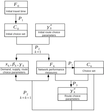
Figure 1 gives a flow chart of the process. Note that all variable subscripts are for iteration numbers, as the variables are already treated as vectors covering all time periods and the time indices are omitted. Note also that inputs to the overall problemP are omitted from the diagram to more clearly present the interactions
between the three sub-problems.
To initialize, choice setsC0are generated based on free flow or static traffic
as-signment link travel timesF0. A base route choice model is assumed with a simple
utility function specification, e.g., one that only includes the travel time as the ex-planatory variable. The a priori parameter valuesγa
0 are assumed based on existing
empirical studies in the literature, rather than estimated from the disaggregate route choice observations. The aggregate calibration problemP2is then solved, and the
iteration counter k is set to 1. Outputs from P2 include the calibrated OD trips xk, supply parametersβk, route choice parameters γk, and network performance
measuresFk. Choice sets are then updated according to Ck = P1(G; Fk). The
disaggregate estimation problemP3 is then solved based on the newly generated
choice setsCkand performance measuresFk. The estimated route choice
param-eters are then used as the a priori valuesγa
kfor the aggregate calibration problem P2 in the next iterationk = k + 1. The iteration continues until a convergence is
reached, usually measured as the relative difference between the time-dependent link travel times from two consecutive iterations.
2.2.1 Choice Set Generation and Evaluation
The route choice set generation problem (P1) takes the network topology and
performance measures as inputs and generates a choice set of alternative paths between each OD pair. The choice set generation algorithms can be classified into two groups: deterministic and stochastic.
Deterministic approaches include the link elimination and link penalty algo-rithms. In the link elimination algorithm, the shortest path is first found between a pair of OD. Then for each link in the shortest path, the algorithm will remove it from the network, find a new shortest path, test it for uniqueness and store it in the choice set if it is unique.
As the link elimination algorithm only removes one link at each iteration, it is possible that the newly generated path only differs from the original one by a short detour around the removed link, and paths far from the original one are unlikely to be generated. The link penalty algorithm could potentially resolve the problem, where the costs of all links included in the choice set are increased in every iteration until the costs reach a threshold. After the threshold is reached, link costs will be set to the normal values and increased in future iterations, which ensures the diversity of the choice set.
Stochastic approaches include the simulation and doubly stochastic algorithm. The simulation algorithm determines a distribution for the cost of every link in the network, for example, normal distribution. For each joint draw of link costs, a shortest path is generated and incorporated in the choice set if it is unique. The rationale for this method is that travelers might have perception errors of travel times (Burrell; 1968; Daganzo and Sheffi; 1977). The number of samples is pre-determined, and can be adjusted empirically depending on the network settings.
The doubly stochastic algorithm is similar to the simulation algorithm. The cost functions are specified like utilities and both the parameters and the attributes are randomly generated, and minimum cost paths are calculated based on these doubly stochastic generalized costs (Bovy and Fiorenzo-Catalano; 2006).
The evaluation of the generated choice set mainly involves two criteria: cov-erage and computational time. Define overlap as the degree to which a generated
routei matches the observed route.
Overlapi = Li,obs Lobs
= overlap distance between generated and observed paths
distance of observed path
(9) When complete routes are not observable, e.g., those from GPS traces with gaps due to the limitation of time resolution, we calculate the overlap by dividing the overlap distance between generated and actually observed traces by the total length of the observed traces.
Coverage is the percent of observed routes for which a generated route at a specified overlap threshold exists. It represents the quality of the choice set gener-ation algorithm, and high coverage is desired.
For any real life application, the choice set generation problem will be solved for a large number of OD pairs. Furthermore, in the iterative process introduced in Figure 1, the choice set generation problem for many OD pairs (P3) will be solved
multiple times. Therefore the computational efficiency of the algorithm is also an important consideration in its evaluation.
2.2.2 Aggregate Calibration Problem: SPSA
The aggregate calibration problem P2 is a minimization problem where the
evaluation of the objective function requires a simulation run of the DTA model. We use the Simultaneous Perturbation Stochastic Approximation (SPSA) algorithm to solve the problem, which is originally developed by Spall (1998), and later ap-plied to DTA calibration by Balakrishna (2006). The SPSA algorithm is attractive for large problems because of its efficient gradient approximation by perturbing all variables at once. It is also designed for stochastic problems and allows for inputs corrupted by noise, which is usually the case in simulation-based DTA models.
The SPSA algorithm works in an iterative fashion, where at iterationk, a
mov-ing direction from the current solution (the gradient in a gradient-based method) is determined. Letθ be the vector of calibration variables, including the OD trips x, supply parameters β and route choice parameters γ, and the size of θ is n. To
calculate the gradient numerically,n evaluations of the objective function need to
be carried out, which are prohibitively expensive for a real life DTA calibration problem wheren is usually very large. The SPSA algorithm does not calculate the
gradient exactly; instead an approximation is calculated by two perturbations of the parameters. The approximate gradient estimate of theithcalibration variable
at iterationk, denoted as gi(θk), is calculated as follows:
gi(θk) =
z(θk+ ck⊗ ∆k) − z(θk− ck⊗ ∆k) 2cki∆ki
where∆k={∆k1, ∆k2, ...∆kn} is generated based on an appropriate random
vari-able distribution, e.g., the Bernoulli distribution, ck={ck1, ck2, ...ckn} is the size
vector for the random perturbation, ⊗ is the component-by-component
multipli-cation of two vectors andz(θ) is the objective function value with the calibration
variable vectorθ.
The gradient approximation at iterationk is then g(θk)={g1(θk), g2(θk), ...gn(θk)},
which only requires two computations of the objective function.
2.2.3 Disaggregate Route Choice Estimation: Latent Choice
Disaggregate route choice models are usually developed under the framework of discrete choice analysis, where a decision maker is assumed to choose from a choice set (see Section 2.2.1) a route with the maximum utility, which is the sum of a function of explanatory variables with unknown parameters and a random term. Parameters of the model are obtained by maximizing the likelihood of observing the chosen routes, namely, solving the problemP3.
Sometimes the chosen routes cannot be unambiguously identified, e.g., when there are large gaps between consecutive GPS readings. In the Beijing case study that will be introduced in detail in Section 3, the GPS readings are at least one minute apart during which the vehicle most likely has traversed multiple links. One solution to this problem is to fill the gaps artificially with shortest paths or other pre-specified types of paths. However, the complete route obtained with this method is not necessarily the real chosen route and may lead to biased estimation. For example, the coefficient of the shortest path dummy in the route choice model would be artificially boosted if we fill these gaps with shortest paths.
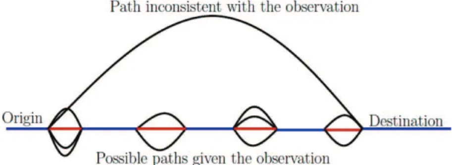
Following Bierlaire and Frejinger (2008), we treat the chosen routes as latent that are not observable. The estimation problem is then based on the observed GPS traces, defined as a series of links matched from GPS points that are not necessarily connected. Therefore each GPS trace might correspond to multiple routes, and the likelihood of observing a GPS tracer for individual n with a given choice set Cn, Pn(r|Cn) can be written as the sum of likelihoods of observing all paths in the
choice set that are consistent with the trace. Formally,
Pn(r|Cn) = X i∈Cn
Pn(i|Cn)δ(r|i). (11)
i is a route in the choice set, Pn(i|Cn) is the route choice model that predicts the
probability of choosing routei for individual n out of a choice set Cn, andδ(r|i)
is a binary variable, which equals one if routei passes through the links in trace g
tracer corresponds to multiple paths, where purple links are observed and red ones
are gaps.
A path-size Logit is used for predicting route choice probability, that is,
Pn(i|Cn) =
exp(ln(PSi) + Vni) P
j∈Cnexp(ln(PSj) + Vnj)
, (12)
whereVniis the systematic utility of alternativei for individual n, PSi is the path
size of alternativei that describes the level of overlapping of the alternative with
all other alternatives in the choice setCn(Ben-Akiva and Bierlaire; 1999). PSi is
equal to 1 if alternativei does not overlap with any other alternatives, and 1/J if it
completely overlaps withJ −1 other alternatives. This is a deterministic correction
to the IIA problem of a Logit model in predicting choice probabilities of correlated alternatives (Ramming; 2002).
Figure 2: The Latent Choice Problem
3
Case Study
3.1 Introduction
In this section we discuss a case study in the City of Beijing using the frame-work proposed above. We first introduce DynaMIT-P, the DTA model used in this case study, and the network settings in Section 3.2. We then introduce the data pro-cessing in Section 3.3. Section 3.4 describes the specific models and algorithms used in the case study under the combined calibration framework, and presents the results in comparison with a previous study where only aggregate calibration was conducted.
3.2 DynaMIT-P and Network Settings
DynaMIT-P (Dynamic Network Assignment for the Management of Informa-tion to Travelers-Planning Version) is a state-of-the-art simulaInforma-tion based DTA sys-tem (Ben-Akiva et al.; 1997, 2001) designed to evaluate Intelligent Transportation Systems at the planning level. With a built-in microscopic demand simulator, a mesoscopic supply simulator, and a learning model to capture the complex inter-actions between traffic demand and supply, it can predict day-to-day evolution of travel demand, network conditions and within-day traffic patterns.
DynaMIT-P and its corresponding real-time version have been applied suc-cessfully in major cities in the US, such as Los Angeles, California (Wen et al.; 2006), Lower Westchester County, New York (Rathi et al.; 2008), and Boston, Massachusetts (Balakrishna et al.; 2008). The Beijing study is, however, the first highly congested urban network DynaMIT-P was applied to. Severe congestion was initially observed in the simulation due to the complexity of network and the large traffic volume. Several enhancements were then done to DynaMIT-P to solve this problem, including enhancing the route choice model from a simple Logit model to a Path-size Logit model, introducing lane groups and variable capacity to the supply model, and doing special treatments to short links to avoid artificial gridlock (Ben-Akiva et al.; 2012).
As shown in Figure 3, the Beijing network consists of a series of ring roads connected by arterial roads with frequent on- and off-ramps. Our study area is the West 2nd Ring Road network and its northern and southern extensions, the area in-cluded in the rectangle. The computer representation of this study network consists of 1,698 nodes connected by 3,129 links. Using results from household surveys, a historical static demand dataset containing 2,927 origin-destination (OD) pairs are generated. The simulation time period is from 6:00:00 am to 10:00:00 am.
3.3 Data
The aggregate surveillance data and GPS vehicle trajectory data were obtained from Beijing Transportation Research Center (BTRC).
3.3.1 Surveillance Data for Aggregate Calibration
We used traffic counts and link travel times from six weekdays during Decem-ber 2007 between 6am and 10am as the surveillance data for aggregate calibration.
The traffic counts were obtained from Remote Traffic Microwave Sensors (RTMS). There were 154 RTMS detectors deployed in our study area and 140 of them were functioning normally to provide traffic flow information continuously. Most of
Figure 3: The study area
them (the triangles shown in Figure 4) were on the expressways. The sensor counts were aggregated with a 15-minute interval by BTRC.
The link travel times were extracted from Floating Car Data (FCD), which were obtained from Global Positioning Systems (GPS) in taxis. FCD cover nearly 90% of all the major roads in Beijing, including arterials and local roads where there is a lack of sensor counts data. The FCD were provided as averages at 5-minute intervals.
3.3.2 GPS Data for Route Choice Estimation
GPS devices installed in taxis in Beijing record the positions and speeds of taxis with a time interval of one minute. BTRC matched the GPS points to certain positions on links. A GPS trace starts when a taxi service begins and ends when the passenger gets off the taxi. A vacant taxi driver’s route choice behavior is conceivably significantly different from a regular driver’s (e.g., circling to look for customers), and thus excluded from the analysis. In general a taxi driver has better spatial knowledge than a regular driver, which might be an important factor in route choice. We focus on the morning peak where the majority of drivers are commuters, who conceivably have good knowledge of their commuting routes. Therefore it is reasonable to use taxi drivers’ data to represent commuters’ behavior
in this particular study. The proposed methodology is not limited and can be easily applied to regular drivers’ data once they are available.
Each GPS entry contains the taxi ID, link ID, time, speed, relative traversed length on the current link, service number and GPS number, which records the order of GPS points within the same service.
In total, we obtained two sets of GPS data from BTRC which spanned nine days. The first set of data includes GPS traces 24 hours/day on two days: April 24, 2008 (Thursday) and April 25, 2008 (Friday). The second set of data includes GPS traces from 6:00am to 10:00am (which matches the DynaMIT-P simulation time) on seven days, May 20, 2008 (Tuesday) through May 23, 2008 (Friday) and May 26, 2008 (Monday) through May 28, 2008 (Wednesday).
Table 1 shows the overall statistics of the GPS data. Table 1: Overall statistics of the GPS data
Number of GPS entries Number of taxis Number of traces 8.9 million 10,412 578,857
As the study area is only a sub-network within the Beijing network, we fil-tered out outside traces and obtained 11,317 traces that were complete in the study area. As DynaMIT-P simulations are from 6:00am to 10:00am, and the time de-pendent travel times used for the route choice model estimation are generated from DynaMIT-P, we only included traces within this time interval in the estimation.
A large number of the traces had very short travel times. Based on practical experience of the local planners from BTRC, an effective taxi trip in Beijing should be more than five minutes in most cases. Therefore, we deleted all the traces shorter than five minutes to ensure a more accurate estimation.
We further eliminated traces that clearly contained mistakes, e.g., Figure 5a shows a GPS trace that may have a GPS mapping mistake as the link with a yellow mark in the middle is directed from the destination to the origin. Figure 5b is an example of those GPS traces that make no sense and for which we cannot find any convincing explanation.
We finally obtained 1,097 consistent and reasonable traces within the simula-tion time period for the route choice model estimasimula-tion. Figure 6 details the spatial distribution of the traces. From left to right, the first three pictures show the 100, 200, 500 most frequently used links and the fourth one shows all the links that were included. The traces concentrated in the northern part, which is reasonable since that is the most congested area. Meanwhile, the traces covered almost the complete network and were deemed adequate to reflect the route choice behavior in the whole study area.
(a) A possible GPS mismatch (b) A trace with mistakes
Figure 5: Unreasonable GPS traces
3.4 The Combined Calibration of DynaMIT-P
3.4.1 Initial Aggregate Calibration
In our previous study (Ben-Akiva et al.; 2012), the DynaMIT-P Beijing model had been calibrated using the SPSA algorithm against the aggregate surveillance data. The route choice model was a Path-size Logit with only one explanatory vari-able, the time-dependent travel time. Its parameter was calibrated simultaneously with other calibration variables against the aggregate data only. The systematic utility function was not tested or estimated using disaggregate GPS traces, and likely to be oversimplified.
We use this result as the base case to evaluate the calibration improvements from combining the disaggregate route choice estimation with aggregate calibra-tion of DynaMIT-P.
3.4.2 Route choice Set Generation
We simultaneously apply three algorithms in DynaMIT-P to generate the choice set, namely link elimination, simulation and link penalty. Time-dependent link travel times are used instead of static link lengths in the calculation of shortest paths. To capture people’s varying attitudes toward the highway, we implemented a highway bias, namely, multiplying highway link travel times by a certain weight in the generation of a choice set. When the weight is greater than 1, the paths are more likely to include fewer highways. Conversely, when the weight is less than 1, paths including more highways are generated. The link number bias was also introduced to capture people’s attitudes toward intersections, since oftentimes the more intersections in a path, the larger the number of links in the path. This was implemented by adding a constant to each link travel time, and thus a path with a larger number of links would be penalized more. The constant could be adjusted to reflect different levels of bias.
Choice sets of all OD pairs consisted of 48,796 paths. The maximum number of paths in a choice set was 222, with a mean of 27.6 paths per OD pair and a standard deviation of 35.6 paths. The maximum number of paths consistent with the GPS trace for an OD pair was 68, the mean was 3.12, and the standard deviation was 5.8 paths.
The coverage test results are shown in Table 2. The high coverage indicates that the choice set we generated is of high quality and the algorithms we implemented can be trusted to generate choice sets for other OD pairs in the DTA simulation.
Table 2: Coverage tests for the choice set generated by DynaMIT-P
Overlap 100% 90% 80%
Coverage 80.0% 85.9% 91.5%
3.4.3 Route Choice Model Specification and Estimation
We specified and compared several models and finally arrived at the utility function as follows:
Vp=β1· T imeDepedentT ravelT imep+ ln(pathsizep)
+ β2· ShortestP athp+ β3· F astestP athp+ β4· M ostHighwayp
(13) Time-Dependent Travel Time
Based on time-dependent link travel times from the latest DTA run, and con-sidering the start time of each GPS trace, we computed the time-dependent travel time for each path with a unit of 1000 seconds.
Path-size
PS is a number between1/J and 1 where J is the size of the choice set.
When PS is equal to1/J, all alternatives are completely overlapping. When
PS is equal to 1, a path is not overlapping with any other paths. Shortest Path Dummy
This is a dummy variable that is 1 for the path with the least total length among all paths with the same OD pair.
Fastest Path Dummy
This is a dummy variable that is 1 for the path with the lowest average travel time among all paths with the same OD pair.
Most Highway Dummy
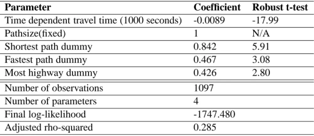
This is a dummy variable that is 1 for the path with the highest ratio of its length spent on the highway, among all paths with the same OD pair. The model is estimated with Biogeme and the estimation result is shown in Table 3.
3.4.4 DTA Re-calibration and Iteration
We implemented the estimated route choice model in DynaMIT-P and ran SPSA calibration again for this new model. With the newly calibrated output travel
Table 3: The result of route choice model estimation
Parameter Coefficient Robust t-test
Time dependent travel time (1000 seconds) -0.0089 -17.99
Pathsize(fixed) 1 N/A
Shortest path dummy 0.842 5.91 Fastest path dummy 0.467 3.08 Most highway dummy 0.426 2.80 Number of observations 1097
Number of parameters 4
Final log-likelihood -1747.480 Adjusted rho-squared 0.285
times from DynaMIT-P, we generated a new choice set and estimated a new route choice model based on the latest choice set and travel times. continued carrying out the iterations as described in Section 2, until the output travel times of the two consecutive aggregate calibrations are close enough.
Table 4 shows the route choice model in the DynaMIT-P base model and the route choice model of our final calibrated model.
Table 4: The route choice model in DynaMIT-P base model and final calibrated model
Parameter Base model Final calibrated model
Time-dependent travel time -0.0183 -0.011 Path-size 1.00(fixed) 1.00(fixed) Shortest path dummy N/A 0.893 Fastest path dummy N/A 0.504 Most highway dummy N/A 0.345
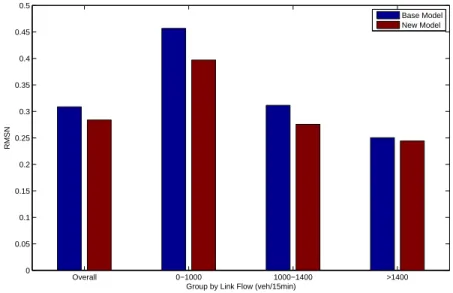
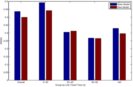
Figure 7 compares the RMSN (Root mean squared errors normalized) for counts from the base case and combined calibration. The first (leftmost) group is the over-all calibration result, and other three groups are links with high flows (more than 1400veh/15min), medium flows (1000-1400 veh/15min) and low flows (0-1000 veh/15min) respectively. We can see more improvements on links with low and medium flows than high flows. Figure 8 compares the RMSN for observed link travel times from FCD in the base case and combined calibration. The first group is the overall calibration result, and there are four groups according to the link travel time: 0-20 seconds, 20-40 seconds, 40-60 seconds and more than 60
sec-onds. We can see more improvements in links with very short and very long travel times. Overall 0−1000 1000−1400 >1400 0 0.05 0.1 0.15 0.2 0.25 0.3 0.35 0.4 0.45 0.5
Group by Link Flow (veh/15min)
RMSN
Base Model New Model
Figure 7: Fit to Counts Statistics of the Base Case (Blue) and Combined Calibra-tion (Red)
The overall calibration results are also reported in Table 5. The improvement in RMSN for counts is 7.8% and the improvement in RMSN for floating car travel time is 8.3%. The improvement could have been larger considering the following facts:
• Compared to the scale of the network, the number of sensors is very limited
(only around 120 sensors). At the same time, the distribution of these sen-sors is limited to expressways, which leads to a failure in capturing possible significant improvements in other type of roads in the network.
• The route choice model specification is still simple. Only three more dummy
variables are included compared to the base model. A route choice model that captures more influencing factors could possibly make further improve-ments, for example, the reliability of travel time. However the calculation of reliability measures require data to derive travel time probabilistic dis-tributions, which are not yet available from the project. It also calls for a potential significant change to the DTA model to explicitly treat travel times as random variables, which will be included in our future work.
Overall 0−20 20−40 40−60 >60 0 0.05 0.1 0.15 0.2 0.25 0.3 0.35 0.4 0.45 0.5
Group by Link Travel Time (s)
RMSN
Base Model New Model
Figure 8: Fit to FCD Link Travel Time Statistics of the Base Case (Blue) and Combined Calibration (Red)
Table 5: Comparisons of Overall Calibration Results
No. of Observations RMSE RMSN Counts(Veh/15min) Base Case 1,680 383.8 0.308
Combined Calibration 353.1 0.284 Travel Time(s) Base Case 52,545 17.30 0.436 Combined Calibration 15.85 0.400
For a closer look, Figure 9 gives the fit-to-count comparison between the base case and the combined calibration during the peak period of 8:30AM-8:45AM for a specific count station. The x-axis is the observed sensor counts and the y-axis is the simulated ones. A 45-degree line indicates a perfect match between the observed and the simulated data, and the closer the dots are to the 45-degree line the better the fit. We can see that the combined calibration gives better fit than the base case.
Figure 9: Fit-to-count Comparison between the Base Model and the New Model
4
Conclusions and Future Directions
In this paper, we extend on the framework of simultaneous demand-supply DTA calibration based on aggregate observations, and incorporate the disaggregate route choice observations to improve the calibration accuracy. We formulate the calibration problem as a bi-level constrained optimization problem. The objective function is a weighted sum of distances between time-dependent location-specic simulated aggregate measurements and eld aggregate measurements (e.g., counts, speeds, and link travel times) and distances between calibrated variable values and their respective a priori values. Constraints include (1) a simulation-based equilib-rium DTA model; (2) a choice set generation model; (3) upper and lower bounds on OD trips and supply/demand parameters; (4) the physical relationships between the model parameters; (5) the route choice estimation problem, where the likelihood of observing the disaggregate route observations (e.g. from GPS traces) is maxi-mized. A priori values of route choice parameters are derived from the lower level
route choice estimation problem. The likelihood function is based on a discrete choice model with route choice sets and attributes generated from performance measures.
The bi-level calibration/estimation problem is solved by an iterative process that alternates between three sub-problems: the upper and lower level problems and the choice set generation model. A case study is conducted in the City of Bei-jing using DynaMIT-P, a state-of-the-art simulation-based DTA model, using the proposed methodology. The SPSA algorithm is used in the aggregate calibration process. A Path-size Logit route choice model is estimated using the disaggregate GPS trajectories and a latent choice model is implemented considering the discon-tinuity of the GPS data. The utility function specification includes time-dependent travel time, Path Size, shortest path dummy, fastest path dummy and most high-way dummy. Compared to the base case where only aggregate surveillance data are used, the combined calibration shows an improved accuracy in terms of fit to observed link flow and link travel time data. Better data and better designed route choice model specification may help in achieving more significant enhancement.
In future work, the framework can be extended to incorporate more types of data other than disaggregate trajectories and aggregate traffic data. For example, with the development of data mining technologies, online social networking web-sites could be analyzed and provide information for deriving traffic demand, es-pecially when special events take place. How to fuse data from different sources with different forms and provide a consistent calibration of DTA models will be a challenging, yet meaningful topic.
References
Antoniou, C. (2004). On-line Calibration for Dynamic Traffic Assignment, PhD thesis, Massachusetts Institute of Technology.
Azevedo, J., Costa, M. S., Madeira, J. S. and Martins, E. V. (1993). An algorithm for the ranking of shortest paths, European Journal of Operational Research
69: 97–106.
Balakrishna, R. (2006). Off-line Calibration of Dynamic Traffic Assignment
Mod-els, PhD thesis, Massachusetts Institute of Technology.
Balakrishna, R., Ben-Akiva, M. and Koutsopoulos, H. N. (2007). Offline calibra-tion of dynamic traffic assignment: Simultaneous demandand- supply estima-tion, Transportation Research Record: Journal of the Transportation Research
Balakrishna, R., Koutsopoulos, H. N. and Ben-Akiva, M. (2005). Calibration and validation of dynamic traffic assignment systems, in H. S. Mahmassani (ed.),
Transportation and Traffic Theory: Flow, Dynamics and Human Interaction, Proceedings of the 16th International Symposium on Transportation and Traffic Theory, Elsevier, University of Maryland, College Park, pp. 407–426.
Balakrishna, R., Morgan, D., Slavin, H. and Yang, Q. (2009). Large-scale traffic simulation tools for planning and operations management, 12th IFAC
Sympo-sium on Transpotaton Systems .
Balakrishna, R., Wen, Y., Ben-Akiva, M. and Antoniou, C. (2008). Simulation-based framework for transportation network management for emergencies,
Transportation Research Record: Journal of the Transportation Research Board
2041: 80–88.
Barcelo, J. and Casas, J. (2006). Stochastic heuristic dynamic assignment based on aimsun microscopic traffic simulator, Transportation Research Record: Journal
of the Transportation Research Board 1964: 70–80.
Ben-Akiva, M., Bergman, M., Daly, A. and Ramaswamy, R. (1984). Modeling in-ter urban route choice behaviour, Proceeding of the 9th Inin-ternational Symposium
on Transportation and Traffic Theory.
Ben-Akiva, M. and Bierlaire, M. (1999). Discrete choice methods and their appli-cations to short-term travel decisions, in R. Hall (ed.), Handbook of
Transporta-tion Science, Kluwer, pp. 5–34.
Ben-Akiva, M., Bierlaire, M., Bottom, J., Koutsopoulos, H. N. and Mishalani, R. G. (1997). Development of a route guidance generation system for real-time application, Proceedings of the 8th International Federation of Automatic
Control Symposium on Transportation Systems, IFAC, Chania, Greece.
Ben-Akiva, M., Bierlaire, M., Burton, D., Koutsopoulos, H. N. and Mishalani, R. (2001). Network state estimation and prediction for real-time transportation management applications, Networks and Spatial Economics 1: 291–318. Ben-Akiva, M., Bottom, J., Gao, S., Koutsopoulos, H. N. and Wen, Y. (2007).
Towards disaggregate dynamic travel forecasting models, Tsinghua Science and
Technology 12(2): 115–130.
Ben-Akiva, M. E., Gao, S., Wei, Z. and Wen, Y. (2012). A dynamic traffic assign-ment model for highly congested urban networks, Transportation Research Part
Ben-Akiva, M. and Lerman, S. (1985). Discrete Choice Analysis, MIT Press. Bierlaire, M. and Frejinger, E. (2008). Route choice modeling with network-free
data, Transportation Research Part C 16: 187–198.
Bolduc, D. and Ben-Akiva, M. (1991). A multinomial probit formulation for large choice sets, Proceedings of the 6th International Conference on Travel
Behaviour.
Bovy, P. H. L. and Fiorenzo-Catalano, S. (2006). Stochastic route choice set gen-eration: behavioral and probabilistic foundations, Proceedings of the 11th
Inter-national Conference on Travel Behaviour Research, Kyoto, Japan.
Burrell, J. E. (1968). Multiple route assignment and its application to capacity restraint, Proceeding of the Fourth International Symposium on the Theory of
Traffic Flow.
Cascetta, E. (2001). Transportation Systems Engineering: Theory and Methods, Applied optimization, Kluwer Academic Publishers, Dordrecht; Boston, MA. Cascetta, E., Nuzzolo, A., Russo, F. and Vitetta, A. (1996). A modified logit route
choice model overcoming path overlapping problems: Specification and some calibration results for interurban networks, in J. B. Lesort (ed.), Proceedings of
the 13th International Symposium on Transportation and Traffic Theory, Lyon,
France.
Daganzo, C. F. and Sheffi, Y. (1977). On stochastic models of traffic assignment,
Transportation Science 11(3): 253–274.
de la Barra, T., P´erez, B. and A ˜nez, J. (1993). Multidimensional path search and assignment, Proceedings of the 21st PTRC Summer Meeting, pp. 307–319. Florian, M., Mahut, M. and Tremblay, N. (2001). A hybrid
optimization-mesoscopic simulation dynamic traffic assignment model, Proceeding of the
In-ternational IEEE Conference on Intelligent Transportation Systems, Oakland,
CA, Aug. 25-29, pp. 118–121.
Fosgerau, M., Frejinger, E. and Karlstrom, A. (2012). A logit model for the choice among infinitely many routes in a network, Technical report, Royal Institute of Technology.
Frejinger, E. (2007). Route choice analysis: Data, models, algorithms and
Frejinger, E. and Bierlaire, M. (2007). Capturing correlation with subnetworks in route choice models, Transportation Research Part B 41: 363–378.
Frejinger, E., Bierlaire, M. and Ben-Akiva, M. (2009). Sampling of alternatives for route choice modeling, Transportation Research Part B 43(10): 984–994. Gao, S. (2005). Optimal Adaptive Routing and Traffic Assignment in Stochastic
Time-Dependent Networks, PhD thesis, MIT.
Hou, A. (2010). Using gps data in route choice analysis: Case study in boston, Master’s thesis, Massachusetts Institute of Technology.
Mahmassani, H. S. (2001). Dynamic network traffic assignment and simulation methodology for advanced system management applications, Networks and
Spa-tial Economics 1(3/4): 267–292.
Peeta, S. and Ziliaskopoulos, A. K. (2001). Foundations of dynamic traffic as-signment: The past, the present and the future, Networks and Spatial Economics
1(3/4): 233–265.
Prato, C. G. (2004). Latent Factors and Route Choice Behavior, PhD thesis, Po-litecnico di Torio.
Ramming, S. (2002). Network knowledge and route choice, PhD thesis, Mas-sachusetts Institute of Technology, Cambridge, MA.
Rathi, V., Antoniou, C., Wen, Y., Ben-Akiva, M. and Cusack, M. (2008). As-sessment of the impact of dynamic prediction-based route guidance using a simulation-based, closed-loop framework, the 87th annual meeting of the
Trans-portation Research Board, DVD-ROM, Washington, D.C.
Spall, J. C. (1998). Implementation of the simultaneous perturbation algorithm for stochastic approximation, IEEE Transactions on Aerospace and Electronic
Systems 34: 817–823.
Sundaram, S., Koutsopoulos, H. N., Ben-Akiva, M., Antoniou, C. and Balakrishna, R. (2011). Simulation-based dynamic traffic assignment for short-term planning applications, Simulation Modelling Practice and Theory 19: 450–462.
Train, K. (2003). Discrete Choice Methods with Simulation, Cambridge University Press.
Vaze, V., Antoniou, C., Wen, Y. and Ben-Akiva, M. (2009). Calibration of dynamic traffic assignment models with point-to-point traffic surveillance, Transportation
Wen, Y. (2009). Scalability of Dynamic Traffic Assignment, PhD thesis, Mas-sachusetts Institute of Technology.
Wen, Y., Balakrishna, R., Ben-Akiva, M. and Smith, S. (2006). Online deployment of Dynamic Traffic Assignment: architecture and run-time management, IEE
Proceedings Intelligent Transport Systems 153(1): 76–84.
Yai, T., Iwakura, S. and Morichi, S. (1997). Multinomial probit with structured co-variance for route choice behavior, Transportation Research Part B 31(3): 195– 207.
Ziliaskopoulos, A. K., Waller, S. T., Li, Y. and Byram, M. (2004). Large-scale dynamic traffic assignment: Implementation issues and computational analysis,