Dynamic vehicle routing for data gathering in wireless networks
The MIT Faculty has made this article openly available.
Please share
how this access benefits you. Your story matters.
Citation
Celik, G.D., and E. Modiano. “Dynamic vehicle routing for data
gathering in wireless networks.” Decision and Control (CDC), 2010
49th IEEE Conference on. 2010. 2372-2377. ©2010 IEEE
As Published
http://dx.doi.org/10.1109/CDC.2010.5717960
Publisher
Institute of Electrical and Electronics Engineers
Version
Final published version
Citable link
http://hdl.handle.net/1721.1/66205
Terms of Use
Article is made available in accordance with the publisher's
policy and may be subject to US copyright law. Please refer to the
publisher's site for terms of use.
Dynamic Vehicle Routing for Data Gathering in Wireless Networks
G¨uner D. C
¸ elik and Eytan Modiano
Abstract— We consider a dynamic vehicle routing problem
in wireless networks where messages arriving randomly in time and space are collected by a mobile receiver (vehicle or a collector). The collector is responsible for receiving these messages via wireless communication by dynamically adjusting its position in the network. Our goal is to utilize a combination of wireless transmission and controlled mobility to improve the delay performance in such networks. We show that the necessary and sufficient condition for the stability of such a
system is given by ρ <1 where ρ is the average system load. We
derive a fundamental lower bound for the delay in the system.
We develop algorithms that are stable for all loads ρ <1 and
that have asymptotically optimal delay scaling. We show that the combination of mobility and wireless transmission results in
a delay scaling ofΘ(1−ρ1 ) with the system load ρ in contrast to
theΘ( 1
(1−ρ)2) delay scaling in the corresponding system where
the collector visits each message location.
Index Terms— Controlled Mobility, Dynamic Vehicle
Rout-ing, TSPN, Data GatherRout-ing, Stability, Delay.
I. INTRODUCTION
There has been a significant amount of interest in perfor-mance analysis of mobility assisted wireless networks in the last decade (e.g., [15], [24]–[28]). Typically, throughput and delay performance of networks were analyzed where nodes moving according to a random mobility model were utilized for relaying data (e.g., [14], [15], [22]). More recently, networks deploying nodes with controlled mobility have been considered focusing primarily on route design and ignoring the communication aspect of the problem (e.g., [9], [27], [28]). In this paper we explore the use of controlled mobility and wireless transmission in order to improve the delay performance of wireless networks.
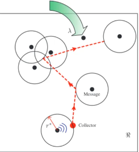
Our model consists of a collector that is responsible for gathering messages that arrive randomly in time at uniformly distributed geographical locations as shown in Fig. 1. The messages are transmitted when the collector is within their communication distance and depart the system upon success-ful transmission. The collector adjusts its position in order to receive these messages in the least amount of time. This setup is applicable to networks deployed in a large area so that a mobile element is necessary to provide connectivity between spatially separated entities in the network. For instance, this setup models a sensor network where a mobile base station collects data from a large number of sensors deployed at random locations inside the network [9], [26], [28]. Another application is utilizing Unmanned Aerial Vehicles (UAVs) as data harvesting devices or as communication relays on
This work was supported by NSF grants 0626781 and CNS-0915988, and by ARO Muri grant number W911NF-08-1-0238.
G ¨uner D. C¸ elik and Eytan Modiano are with Massachusetts Institute of Technology (MIT),{gcelik, modiano}@mit.edu
Collector
ℜ r∗
Message
λ
Fig. 1. The collector adjusts its position in order to receive randomly arriving messages via wireless communication. The circles with radius r∗represent the communication range and the dashed lines represent the
collector’s path.
a battlefield environment [24]. This model also applies to networks in which data rate is relatively low so that data transmission time is comparable to the collector’s travel time, for instance in underwater sensor networks [1].
Vehicle Routing Problems (VRPs) have been extensively studied in the past (e.g., [4], [6], [7], [12], [20], [27]). The common example of a VRP is the Euclidean Traveling Salesman Problem (TSP) in which a single server is to visit each member of a fixed set of locations on the plane such that the total travel cost is minimized. Several extensions of TSP have been considered in the past such as stochastic demand arrivals and the use of multiple servers [6], [7], [12]. In particular, in the TSP with neighborhoods (TSPN) problem the vehicle is to visit a neighborhood of each demand loca-tion [4], [20], which can model a mobile collector receiving messages from a communication distance. A more detailed review of the literature in this field can be found in [7], [20]. Of particular relevance to us among the VRPs is the Dynamic Traveling Repairman Problem (DTRP) due to Bertsimas and van Ryzin [6], [7], [8]. DTRP is a stochastic and dynamic VRP in which a vehicle is to serve demands that arrive randomly in time and space. Fundamental lower bounds on delay were established and several vehicle routing policies were analyzed for DTRP for a single server in [6], for multiple servers in [7] and for general arrival and service distributions in [8]. This model was generalized to the Dynamic Pickup and Delivery Problem (DPDP) in [27] where fundamental bounds on delay were established. We apply this model to wireless networks where the demands are data messages to be transmitted to a collector which is
49th IEEE Conference on Decision and Control December 15-17, 2010
capable of wireless communication1. In our system the prob-lem has considerably different characteristics since in this case the collector does not have to visit message locations but rather can receive the messages from a distance using wireless communication. The objective in our system is to effectively utilize this combination of wireless transmission and controlled mobility in order to minimize the time average message waiting time.
In a closely related problem where multiple mobile nodes with controlled mobility and communication capability relay the messages of static nodes with saturated arrivals, [25] derived a lower bound on node travel times. In an indepen-dent work, [18] considered utilizing mobile wireless servers as data relays on periodic routes and applied various delay relations from Polling models to this setup. A mobile server harvesting data from spatial queues in a wireless network was considered in [24] where the stability region of the system was characterized using a fluid model approximation. A similar model where the messages are transmitted according to a random access scheme creating interference among neighboring transmissions is analyzed in [10]. In this paper the message transmissions are scheduled, i.e., there is only one transmission in the system at a given time.
Another related body of literature lies in the area of utilizing mobile elements that can control their mobility to collect sensor data in Delay Tolerant Networks (DTN) (e.g., [9], [26], [28]). Route selection (e.g., [26]), scheduling or dynamic mobility control (e.g., [9], [28]) algorithms were proposed to maximize network lifetime, to provide connec-tivity or to minimize delay. These works focus primarily on mobility and usually consider particular policies for the mobile element. To the best of our knowledge, this is the first attempt to develop fundamental bounds on delay in a system where a collector is to gather data messages randomly arriving in time and space using wireless communication and
controlled mobility.
The main contributions of this work are the following. We show thatρ < 1 is the necessary and sufficient condition for the stability of the system where ρ is the system load. We derive fundamental lower bounds on delay and develop algorithms that have asymptotically optimal delay scaling. We show that the combination of mobility and wireless transmission results in a delay scaling of Θ(1/(1 − ρ)) in contrast to theΘ(1/(1 − ρ)2) delay scaling in the system in
[6] where the collector visits each message location. This paper is organized as follows. In Section II we describe the system model and in Section III we characterize the necessary and sufficient conditions for the stability of the system. We derive a lower bound on delay in Section IV and in Section V we provide upper bounds on delay together with numerical results.
1In [6], [7], or [8] the collector needs to be at the message location in
order to be able to serve it, therefore, we will refer to the DTRP model as the system without wireless transmission.
II. MODEL
Consider a square region R of area A and messages arriving into R according to a Poisson process (in time) of intensity λ. Upon arrival the messages are distributed independently and uniformly inR and they are to be gathered by a collector via wireless reception. An arriving message is transmitted to the collector when the collector comes within the reception distance of the message location and grants access for the message’s transmission. Therefore, there is no interference power from the neighboring nodes during message receptions. We assume that the transmit power PT is constant and that the transmissions are subject to
distance attenuation. In such a system, the received power of a transmission from nodei, located at distance ri from
the collector, is given byPR,i= PTKr−αi [15], [16], where
α is the power loss exponent (typically between 2 and 6), andK is the attenuation constant normalized to 1.
Next we argue that the Signal to Noise Ratio (SNR) packet reception model [15], [16] is equivalent to a disk model [10], [16] under the above assumptions. In the SNR model, a transmission is successfully decoded at the collector if its SNR is above a thresholdβ, i.e., if SNRi = PR,i/PN ≥ β,
where PN is the background noise power. We let r be
the reception distance of the collector. If the location of the next message to be received is within r, the collector stops and attempts to receive the message. Otherwise, the collector travels towards the message location until it is within a distancer away from the message. A transmission at distancer to the collector is successful if r ≤ (SNRc/β)1/α
where SNRc = PT/PN denotes the SNR of a transmission
from unit distance. Therefore, the optimal reception distance is the maximum reliable communication distance r∗ =
(SNRc/β)1/α. Hence, essentially we have a disk model of
radiusr∗, where a transmission can be received only if it is
within a disk of radius r∗ around the collector. Under this
model, transmissions are assumed to be at a constant rate taking a fixed amount of time denoted bys.
The collector travels from the current message reception point to the next message reception point at a constant speed v. We assume that at a given time the collector knows the locations and the arrival times of the messages that arrived before this time. The knowledge of the service locations is a standard assumption in vehicle routing literature [4], [6], [12], [20], [27]. Let N (t) denote the total number of messages in the system at timet. We say that the system is stable under a policy if [3], [21],
lim sup
t→∞ E[N (t)] <∞, (1)
namely, the long term expected number of messages in the system is finite. Let ρ = λs denote the load arriving into the system per unit time. For stable systems,ρ denotes the fraction of time the collector spends receiving messages.
III. STABILITY
In this section we characterize a necessary and sufficient condition for the stability of the system. LetW denote the total time average waiting time per message.
A. Necessary Condition for Stability
Theorem 1: A necessary condition for the stability of any policy isρ < 1. Furthermore, we have
W ≥ λs
2
2(1 − ρ). (2)
Proof: We use the following lemma to bound the delay.
Lemma 1: The steady state time average delay in the system under any policy φ is at least as big as the delay
of any work-conserving2 policy in the equivalent system in which travel times are zero (i.e.,v = ∞).
The proof is omitted due to brevity3 but it is based on an induction argument that the total number of messages in the system is always greater than that in the infinite velocity system. This is because the service time per message is greater than that in the infinite velocity system. Since the latter system behaves as an M/D/1 queue (a queue with Poisson arrivals, constant service times and 1 server), its average waiting time is given by the Pollaczek-Khinchin (P-K) formula for M/G/1 queues [5, p. 189], given in (2). A direct consequence of this lemma is that a necessary condition for stability in the infinite velocity system is also necessary for our system. The necessary and sufficient condition for stability in an M/G/1 queue is given byρ < 1 (see e.g., [5] or [13]).
B. Sufficient Condition for Stability
Here we prove that ρ < 1 is a sufficient condition for stability of the system under a policy based on Euclidean TSP with neighborhoods (TSPN). TSPN is a generalization of TSP in which the server is to visit a neighborhood of each demand location via the shortest path [4], [20]. In our case the neighborhoods are disks of radiusr∗ around each
message location. TSPN is an NP-Hard problem such as TSP. Recently, [20] proved that a Polynomial Time Approximation Scheme (PTAS) exists for TSPN among fat regions in the plane. A region is said to be fat if it contains a disk whose size is within a constant factor of the diameter of the region, e.g., a disk, and a PTAS belongs to a family of (1 + ǫ)-approximation algorithms parameterized by ǫ > 0.
1) TSPN Policy: Assume the system is initially empty (at time t0 = 0). The receiver waits at the center of R
until the first message arrival, moves to serve this message and returns to the center. Let time t1 be the time at which
the receiver returns to the center. At t1, if the system is
empty, the receiver repeats the above process and we define t2 similarly. If there are messages waiting for service at
time t1, the receiver computes the TSPN tour (e.g., using
the PTAS in [20]) through all the messages that are present in the system at timet1, receives these messages in that tour
and returns to the center. We let t2 > t1 be the first time
when the receiver returns to the center after receiving all the messages that were present in the system at t1 and repeat
the above process. We define the epochsti as the time the
2A work-conserving policy is such that the server does not idle when the
queue is not empty.
3Note that all the proofs can be found in our technical report [11].
receiver returns to the center after serving all the messages that were present in the system at timeti−1 4.
Let the total number of messages waiting for service at time ti, Ni , N(ti), be the system state at time ti. Note
thatNiforms an irreducible Markov chain on countable state
space N. We show the stability of the TSPN policy through the ergodicity of this Markov chain.
Theorem 2: The system is stable under the TSPN policy for all loadsρ < 1.
Proof: Given the system stateNi at timeti, we apply
the algorithm in [20] to find a TSPN tour of lengthLi that
is at most(1 + ǫ) away from the optimal TSPN tour length L∗
i. Note thatL∗i can be upper bounded by a constantL for
allNi. This is because the collector does not have to move
for messages within its communication range and a finite number of such disks of radius r∗ can cover the network
region for any r∗ > 0. The collector then can serve the
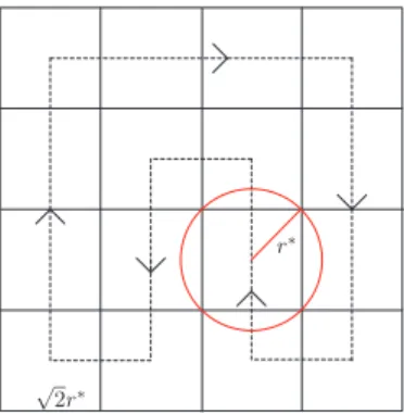
messages in each disk from its center (an example of such a tour is shown in Fig. 2). We will use the Lyapunov-Foster criterion to show that the Markov chain described by the statesNi is positive recurrent [3]. We useV (Ni) = sNi, the
total load served duringithcycle, as the Lyapunov function
(note that V (0) = 0, Sk = {x : V (x) ≤ K} is a bounded
set for all finite K and V (.) is a non-decreasing function). Since the arrival process is Poisson, the expected number of arrivals during a cycle can be upper-bounded as follows:
E[Ni+1|Ni] ≤ λ(L/v + sNi). (3)
Hence we obtain the following drift expression for the load during a cycle.
E[sNi+1− sNi|Ni] ≤ ρL/v − (1 − ρ)sNi.
Sinceρ < 1, there exist a δ > 0 such that ρ + δ < 1: E[sNi+1− sNi|Ni] ≤ ρL/v − δsNi
≤ −δs + ρLv .1{Ni∈S}, (4) where 1{N∈S} is equal to 1 if N ∈ S and zero otherwise
and S = {N ∈ N : N ≤ K} is a bounded set with K = ⌈vδsρL+1⌉. Hence the drift is negative as long as Niis outside
a bounded set. Therefore, by the standard Lyapunov-Foster criterion [2], [3], the Markov chain(Ni) is positive recurrent,
it has a unique stationary distribution and we can bound the steady state time average of Ni as [21]
lim sup
ti→∞
E[N (ti)] ≤ λL
v(1 − ρ). (5)
Furthermore, given somet ∈ [ti, ti+1], we have
lim sup
t→∞ E[N (t)] ≤ lim supti→∞
E[N (ti) + N (ti+1)]
≤ 2 λL
v(1 − ρ)< ∞. (6)
4A similar policy based on TSP was discussed in [23] for a system without
communication capability, where the average delay was characterized for the heavy load regime.
The delay scaling of the TSPN policy with load ρ is 1−ρ1 as shown in (6), the same delay scaling as in a G/G/1 queue. This is a fundamental improvement in delay due to the communication capability as the system without wireless transmission in [6] hasΘ( 1
(1−ρ)2) delay scaling.
Note that ρ < 1 is a sufficient stability condition also for the system without communication capability. This case corresponds tor∗= 0, where we utilize a (1 + ǫ) PTAS for
the optimal TSP tour through the message locations instead of the TSPN tour. An upper bound on the TSP tour for any Nipoints arbitrarily distributed in a square of areaA is given
by√2ANi+1.75
√
A [19]. Similar arguments as above leads to the drift condition
E[sNi+1− sNi|Ni] ≤ ρ(κ1pANi+ κ2) − (1 − ρ)sNi,
for some constants κ1 and κ2, where the drift is again
negative as long as Ni is outside a bounded set S. The
difference in this case is that the travel time per cycle scales with the number of messagesNias√Niwhich can be shown
to result inO((1−ρ)1 2) delay scaling with the load ρ. IV. LOWERBOUNDONDELAY
For wireless networks with a small area and/or very good channel quality such that r∗ ≥ pA/2, the collector does
not need to move as every message will be in its reception range if it just stays at the center of the network region. In that case the system can be modeled as an M/D/1 queue with service time s and the associated queuing delay is given by the P-K formula for M/G/1 queues, i.e., W = λs2/(2(1 − ρ)). However, when r∗ <pA/2, the collector
has to move in order to receive some of the messages. In this case the reception time s is still a constant, however, the travel time per message is now a random variable which is not independent over messages (for example, observing small travel times for the previous messages implies a dense network, and hence the future travel times per message are also expected to be small). Next we provide a lower bound similar to a lower bound in [6] with the added complexity of communication capability in our system.
Theorem 3: The optimal steady state time average delay
T∗ is lower bounded by5 T∗≥E[(||U|| − r∗) +] v(1 − ρ) + λs2 2(1 − ρ)+ s. (7)
The proof is omitted due to brevity but below we give its outline. LetTi, Ti,r− Ti,abe the time between the arrival
of message i at Ti,a and its reception at Ti,r. Ti has three
components: Messagei’s service time s and Wd,i andWs,i,
the waiting times due to the collector’s travel and collector’s packet receptions from the timeTi,a until the time Ti,r− s.
The total waiting time of message i is denoted by Wi =
Wd,i+ Ws,i, henceWi = Ti− s. The time average waiting
time of messagei is defined by an expectation in the steady state given byW = limi→∞E[Wi]. The time average delays
T , WdandWsare defined similarly to haveT = Wd+Ws+s
5Note that
(||U|| − r∗)+ represents max(0, ||U|| − r∗) and U is a
uniformly distributed random variable over the network regionR.
where all the limits are assumed to exist.T∗ is the optimal
system time which is given by the policy that minimizesT . The proof relies on the fact that in a stable system in steady state the average number of messages received in a waiting time is equal to the average number of arrivals in a waiting time given byλW = λ(Wd+Ws). This fact is used to derive
W = Wd
1 − ρ + λs2
2(1 − ρ). (8)
Furthermore,Wdcan be lower bounded by E[(||U|| − r∗)+],
the expected distance of a uniform arrival to the center of the network lessr∗. This is because the center of the square
region R is the best a priori location in the network that minimizes the expected distance to a uniform arrival. Note that the E[(||U|| − r∗)+] term can be further lower bounded
by E[||U||] − r∗, where E[||U||] = 0.383√A [6]. Theorem 3
argues that in addition to the average waiting time of a classical M/G/1 queue given in (2), the queueing delay also increases due to the collector’s travel.
V. COLLECTORPOLICIES
We derive upper bounds on delay via analyzing policies for the collector. The TSPN policy analyzed in Section III-B.1 is stable for all loadsρ < 1 and has O( 1
1−ρ) delay scaling.
Since the lower bound in Section IV also scales with the load as 1−ρ1 , the TSPN policy has optimal delay scaling.
A. First Come First Serve (FCFS) Policy
A straightforward policy is to serve the messages in the order of their arrival times. Specifically, a version of the FCFS policy where the collector returns to the center of the network region (the median of the region for general network regions) after each message reception is shown to be optimal at light loads for the DTRP problem [6]. This is because the center of the network region is the location that minimizes the expected distance to a uniformly distributed arrival. Since in our system we can do at least as good as the DTRP, FCFS policy is optimal also for our system at light loads. Furthermore, the FCFS policy is not stable for all loadsρ < 1, namely, there exists a value ˆρ such that the system is unstable under FCFS policy for all ρ > ˆρ. This is because under the FCFS policy, the average travel component of the service time is fixed, which makes the average arrival rate greater than the average service rate as ρ → 1. Therefore, it is better for a policy to serve more messages in the same “neighborhood” in order to reduce the amount of time spent on mobility.
B. Partitioning Policy
Next we propose a policy based on partitioning the net-work region into subregions and the collector performing a cyclic service of the subregions. This policy is an adaptation of the Partitioning policy of [6] to the case of a system with wireless transmission. We explicitly derive the delay expression for this policy and show that it scales with the load asO(1−ρ1 ) as in the TSPN policy.
r∗
√ 2r∗
Fig. 2. The partitioning of the network region into square subregions of side√2r∗. The circle with radius r∗represents the communication range
and the dashed lines represent the collector’s path.
We divide the network region into(√2r∗x√2r∗) squares
as shown in Fig. 2. This choice ensures us that every location in the square is within the communication distance r∗ of the center of the square. The number of subregions
in such a Partitioning is given by6 ns = A/(2(r∗)2). The
partitioning in Fig. 2 represents the case of ns = 16
subregions. The collector services the subregions in a cyclic order as displayed in Fig. 2 by receiving the messages in each subregion from its center using an FCFS order. The messages within each subregion are served exhaustively, i.e., all the messages in a subregion are received before moving to the next subregion. The collector then receives the messages in the next subregion exhaustively using FCFS order and repeats this process. The distance traveled by the collector between each subregion is a constant equal to √2r∗. It
is easy to verify that the Partitioning policy behaves as a multiuser M/G/1 system with reservations (see [5, p. 198]) where the ns subregions correspond to users and the travel
time between the subregions corresponds to the reservation interval. Using the delay expression for multiuser M/G/1 queue with reservations in [5, p. 200] we obtain,
Tpart= λs2 2(1 − ρ)+ ns− ρ 2v(1 − ρ) √ 2r∗+ s, (9)
whereρ = λs is the system load. Combining this result with (7) and noting that the above expression is finite for all loads ρ < 1, we have established the following observation.
Observation 1: The time average delay in the system scales asΘ(1−ρ1 ) with the load ρ and the Partitioning policy
is stable for allρ < 1.
Despite the travel component of the service time, we can achieveΘ( 1
1−ρ) delay as in classical queuing systems (e.q.,
G/G/1 queue). This is the fundamental difference between this system and the corresponding system where wireless transmission is not used, as in the latter system the delay scaling with load is Θ((1−ρ)1 2) [6]. This difference can be explained intuitively as follows. Denote by N the average number of departures in a waiting time. It is easy to see from the P-K formula that in a classical M/G/1 queue,N scales with the load as Θ(1−ρ1 ). We argue that this scaling for N
6If√n
s is not even or if the subregions do not fit the network region
for a particular choice of r∗, then one can partition the region using the
largest reception distance r∗< r∗such that these conditions are satisfied.
is preserved in our system but not in [6]. The time average waiting time expression as a function of the waiting time due to collector’s travel, Wd, in (8) implies that for any given
policy with its correspondingWd,N can be lower bounded
by λWd
1−ρ. For the system in [6], the minimum per-message
distance the collector moves in the high load regime scales as Ω(√√A
N) [6] (intuitively, the nearest neighbor distance
among N uniformly distributed points on a square region of areaA scales as √√A
N). Therefore, for this system we have
Wd ≈ NΩ( √ A √ N) ≈ Ω( √ N A) which gives N ≈ Ω((1−ρ)λ2A2). Namely, Wd increases with the load and this results in an
extra1/(1 − ρ) scaling in delay in addition to the 1/(1 − ρ) factor of classical M/G/1 queues. However, with the wireless reception capability, the collector does not need to move for messages that are inside a disk of radiusr∗ around it. Since
a finite (constant) number of such disks cover the network region,Wdcan be upper bounded by a constant independent
of the system load (for the Partitioning policy an easy upper bound on Wd is the length of one cyclic tour around the
network). Therefore, in our systemN scales as 1/(1 − ρ) as in classical queues.
In [10] we analyzed the case where the messages were transmitted to the collector using a random access scheme (i.e., with probability p in each time slot) and obtained
Ω( 1
(1−ρ)2) delay scaling as in the system without wireless transmission. The reason for this is that in order to have suc-cessful transmissions under the random access interference of neighboring nodes, the reception distance should be of the same order as the nearest neighbor distances [10], [15].
C. Numerical Results
Here we present numerical results corresponding to the analysis in the previous sections. We lower bound the delay expression in (7) using E[(||U|| − r∗)+] ≥ E[||U||] − r∗
(where E[||U||] = 0.383√A is the expected distance of a uniform arrival to the center of square region of area A [6]). Fig. 3 shows the delay lower bound as a function of the network load for different levels of channel quality7. As
the channel quality increases, the message delay decreases as expected. For heavy loads, the delay in the system is significantly less than the delay in the corresponding system without wireless transmission in [6], demonstrating the difference in the delay scaling between the two systems. For light loads and more noisy communication channels, the delay performance of the wireless network tends to the delay performance of [6].
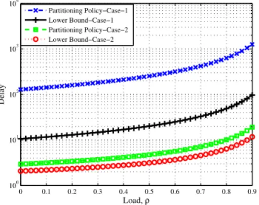
Fig. 4 compares the delay in the Partitioning Policy to the delay lower bound for two different cases. When the travel time dominates the reception time, the delay in the Partitioning policy is about10.6 times the delay lower bound. For a more balanced case, i.e., when the reception time is comparable to the travel time, the delay ratio drops to2.4.
7For the delay plot of the no-communication system, the point that is not
smooth arises since the plot is the maximum of two delay lower bounds proposed in [6].
0 0.2 0.4 0.6 0.8 1 100 101 102 103 104 Load, ρ
Delay Lower Bound
No communication SNR = 30dB SNR = 20dB SNR = 10dB
Fig. 3. Delay lower bound vs. network load using different SNR values for A= 200, β = 2, α = 4, v = 1 and s = 1. 0 0.1 0.2 0.3 0.4 0.5 0.6 0.7 0.8 0.9 100 101 102 103 104 Load, ρ Delay Partitioning Policy−Case−1 Lower Bound−Case−1 Partitioning Policy−Case−2 Lower Bound−Case−2
Fig. 4. Delay in the Partitioning policy vs the delay lower bound for SN Rc= 17dB (r∗= 2.2), β = 2 and α = 4. Case-1: Dominant travel
time (A= 800, v = 1, s = 2). Case-2: Comparable travel and reception times (A= 60, v = 10, s = 2).
VI. CONCLUSION
In this paper we considered the use of dynamic vehicle routing in order to improve the delay performance of wireless networks where messages arriving randomly in time and space are gathered by a mobile collector. We characterized the stability region of this system to be all system loads ρ < 1 and derived fundamental lower bounds on time average expected delay. We derived upper bounds on delay by analyzing policies and extended our results to the case of multiple collectors in the system. Our results show that combining controlled mobility and wireless transmission results in Θ(1−ρ1 ) delay scaling with load ρ. This is the fundamental difference between our system and the system without wireless transmission (DTRP) analyzed in [6] and [7] where the delay scaling with the load is Θ((1−ρ)1 2).
This work is a first attempt towards utilizing a combination of controlled mobility and wireless transmission for data collection in stochastic and dynamic wireless networks. Therefore, there are many related open problems. In this paper we have utilized a simple wireless communication model based on a communication range. In the future we intend to study more advanced wireless communication models such as modeling the transmission rate as a function of the transmission distance. Finally, extending our results for a general message location distribution in the network is
a subject of future research.
REFERENCES
[1] I. F. Akyildiz, D. Pompili, and T. Melodia, “Underwater Acoustic Sensor Networks: Research Challenges,” Ad Hoc Networks (Elsevier), vol. 3, no. 3, pp. 257-279, Mar. 2005.
[2] E. Altman, P. Konstantopoulos, and Z. Liu, “Stability, monotonicity and invariant quantities in general polling systems,” Queuing Sys., vol. 11, pp. 35-57, 1992.
[3] S. Asmussen, “Applied Probability and Queues,” Wiley, 1987. [4] E. M. Arkin and R. Hassin, “Approximation algorithms for the
geometric covering salesman problem,” Discrete Applied Mathematics, vol. 55, pp. 197-218, 1994.
[5] D. Bertsekas and R. Gallager, “Data Networks,” Prentice Hall, 1992. [6] D. J. Bertsimas and G. van Ryzin, “A stochastic and dynamic vehicle routing problem in the Euclidean plane,” Opns. Res., vol. 39, pp. 601-615, 1990.
[7] D. J. Bertsimas and G. van Ryzin, “Stochastic and dynamic vehicle routing in the Euclidean plane with multiple capacitated vehicles,”
Opns. Res., vol. 41, pp. 60-76, 1993.
[8] D. J. Bertsimas and G. van Ryzin, “Stochastic and dynamic vehicle routing with general demand and interarrival time distributions,” Adv.
App. Prob., vol. 20, pp. 947-978, 1993.
[9] B. Burns, O. Brock, and B. N. Levine, “MV routing and capacity build-ing in disruption tolerant networks,” In Proc. IEEE INFOCOM’05, Mar. 2005.
[10] G. D. Celik and E. Modiano, “Random access wireless networks with controlled mobility”, In Proc. IFIP MEDHOCNET’09, Jun. 2009. [11] G. D. Celik and E. Modiano, ”Dynamic Vehicle Routing for
Data Gathering in Wireless Networks”, ArXiv Technical Report, arXiv:1008.4629, Aug. 2010.
[12] E. Frazzoli and F. Bullo, “Decentralized algorithms for vehicle routing in a stochastic time-varying environment,” In Proc. IEEE CDC’04, Dec. 2004.
[13] L. Georgiadis, M. Neely, and L. Tassiulas, “Resource Allocation and Cross-Layer Control in Wireless Networks,” Now Publishers, 2006. [14] A. E. Gammal, J. Mammen, B. Prabhakar, and D. Shah,
“Throughput-delay trade-off in wireless networks,” In Proc. IEEE INFOCOM’04, Mar. 2004.
[15] M. Grossglauser and D. Tse, “Mobility increases the capacity of ad hoc wireless networks ,” IEEE/ACM Trans. Netw., vol. 11, no. 1, pp. 125-137, Feb. 2003.
[16] P. Gupta and P. R. Kumar, “The capacity of wireless networks,” IEEE
Trans. Inf. Theory, vol. 46, no. 2, pp. 388-404, Mar. 2000.
[17] M. Haimovich and T. L. Magnanti, “Extremum properties of of hexag-onal partitioning and the uniform distribution in euclidian location,”
SIAM J. Disc. Math.1, 50-64, 1988.
[18] V. Kavitha and E. Altman, “Queueing in Space: design of Message Ferry Routes in sensor networks,” In Proc. ITC’09, Sep. 2009. [19] E. L. Lawler, J.Lenstra, A. Kan, D. Shmoys, “ The Traveling salesman
problem :a guided tour of combinatorial optimization,” Wiley, 1985. [20] J. S. B. Mitchell, “A PTAS for TSP with neighborhoods among fat
regions in the plane,” In Proc. ACM-SIAM SODA’07, Jan. 2007. [21] E. Modiano, D. Shah and G. Zussman, “Maximizing
through-put in wireless networks via Gossip,” In Proc. ACM
SIGMET-RICS/Performance’06, June 2006.
[22] M. J. Neely and E. Modiano, “ Capacity and delay tradeoffs for ad hoc mobile networks,” IEEE Trans. Inf. Theory, vol. 51, no. 6, pp. 1917-1937, Jun. 2005.
[23] M. Pavone, N. Bisnik, E. Frazzoli and V. Isler, “Decentralized vehicle routing in a stochastic and dynamic environment with customer impatience,” In Proc. RoboComm’07, Oct. 2007.
[24] J. Le Ny, M. Dahleh, E. Feron, and E. Frazzoli, “Continuous Path Planning for a Data Harvesting Mobile Server,” In Proc. IEEE
CDC’08, Dec. 2008.
[25] V. Sharma, E. Frazzoli, and P. G. Voulgaris, “Delay in mobility-assisted constant-throughput wireless networks,” In Proc. IEEE
CDC’05, Dec. 2005.
[26] Y. Shi and Y. T. Hou, “Theoretical results on base station movement problem for sensor network,” In Proc. IEEE INFOCOM’08, Apr. 2008. [27] H. Waisanen, “Control of mobile networks using dynamic vehicle
routing,” Ph.D. Thesis, MIT, 2007.
[28] M. Zhao, M. Ma, and Y. Yang, “Mobile data gathering with space-division multiple access in wireless sensor networks,” In Proc. IEEE
INFOCOM’08, Apr. 2008.