A distributed simulation environment for multibody physics

A Distributed Simulation Environment for

Multibody Physics

by

Jen-Diann Chiou

B.S., Civil Engineering

National Taiwan University, 1992

S.M., Civil and Environmental Engineering

Massachusetts Institute of Technology, 1996

Submitted to the Department of Civil and Environmental Engineering

in partial fulfillment of the requirements for the degree of

Doctor of Philosophy in Information Technology

at the

MASSACHUSETTS INSTITUTE OF TECHNOLOGY

August 1998

@

Jen-Diann Chiou, MCMXCVIII. All rights reserved.

The author hereby grants to MIT permission to reproduce and

distribute publicly paper and electronic copies of this thesis document

in whole or in part.

Author ...

...

...

Department of Civil ald Environmental Engineering

August 14, 1998

Certified by..

/

_{. John R. Williams}

Department of Civil and Environmental Engineering

Thesis Supervisor

Accepted by ...

...

MASSACHUSETTS INSTITUTE Joseph

M. Sussman

OFTECHNOLOGY

_{Chairman, Departmental Committee on Graduate Students}

CT2 6 1998

A Distributed Simulation Environment for Multibody

Physics

by

Jen-Diann Chiou

Submitted to the Department of Civil and Environmental Engineering on August 14, 1998, in partial fulfillment of the

requirements for the degree of

Doctor of Philosophy in Information Technology

Abstract

A distributed simulation environment, which can be used to model multibody physics, is developed. The software design is based on the object oriented paradigm and is implemented in C++ to run on a single workstation or multiple processors in parallel. It provides facilities to set up a multibody physics simulation, including arbitrary 3D geometric representation, particle interactions such as contacts and constraints, and visualization for postprocessing.

Contact detection, the process of automatic identifying the geometric overlap be-tween objects, is generally the most time-consuming procedure in the overall discrete element analysis pipeline. The computational cost of contact detection grows as a function of both the number of particles and the complexity of the geometric repre-sentation of each body. This thesis presents algorithms that significantly reduce the computational cost of the contact detection problem. The hashtable-based spatial reasoning algorithm demonstrates an O(M) performance, where M is the number of particles in the simulation system for a restricted set of particles.

The discrete function representation (DFR) scheme is employed to model the surface geometry of complex 3D objects. DFR-based contact detection between a pair of objects exhibits an O(N) running time performance, where N is the number of surface point used to represent each object. In practice this results in a significant speedup over traditional techniques.

A distributed DEM simulation environment is built on top of a set of software tools which exploit the parallelism embedded in the DEM analysis and which take advantage of a high-speed communications network to achieve good parallel perfor-mance. The goal is of reducing the entire computing time of of large-scale simulation problems to order O(N) is shown to be achieveable using the algorithms described.

Thesis Supervisor: John R. Williams Title: Associate Professor

Acknowledgments

This work would not have been possible without help of many individuals and insti-tutions.

First, I am indebted to my thesis advisor, Professor John R. Williams, for his incessant support, advice, and encouragement.

Professors Jerome Connor, Eduardo Kausel, and Kevin Amaratunga, for their invaluable advice and insight.

I gratefully acknowledge Professors Shang-Hsien Hsieh, Ming-Teh Wang, San-Cheng Chang, and Yeong-Bin Yang, for their encouragement and help.

I deeply appreciate Drs. Ruaidhrl O'Connor and Dale Preece from Sandia Na-tional Laboratories, for their timely guidance, advice, and support.

To Mr. Petros Komodromos, for his help on preparing for the thesis defense. To Mr. Felix Yi-Da Ho and Ms. Sylvia Chao and their family, for their support and taking care of my life here in Cambridge.

To Ms. Tina Lo and her family, for their encouragement and friendship. To Mr. Bang-Yen Lin and his wife Kathy Chen, for their sincere friendship. To Mr. Kenji Iwamoto and colleagues from Kajima Corporation, for giving me the wonderful working experience in Tokyo.

To Ms's Janet Tsai, Faustina Tsai, Chu-Jun Huang, Sandy Lin, and their family, for their friendship and encouragement.

To Ms. Joan McCusker, for her help and taking care of me here in MIT.

To Mr. Petros Komodromos and Ms. Katherine Treash, for their help on preparing for the thesis.

To Ms. Ching-Wen Hsu and her family, for their thoughtfulness and encourage-ment throughout these years.

To Ms's. Jane Chiou and Sylvia Chiou, for their love and help.

This thesis is dedicated to my parents, to whom I owe the most, for their uncon-ditional support and sacrifice over all these years.

Contents

1.4 Computational Requirements in DEM . . . . 1.4.1 Object Representation Requirements . . . . . 1.4.2 Contact Detection Requirements . . . . 1.4.3 Contact Resolution Requirements . . . . 1.4.4 User Interface and Visualization Requirements 1.5 Characteristics of the DEM3D Simulation System .

1.5.1 Basic Functionality . . . . 1.5.2 Object-Oriented Technology . . . . 1.6 Distributed and Parallel Implementation . . . . 1.7 Review of Other DEM Systems . . .... ... 1.8 Thesis Outline . . . ...

2 Algorithms for Spatial Reasoning 2.1 Introduction . ....

2.2 Spatial Sorting Algorithm . . . . 2.2.1 Introduction . . . ... 2.2.2 Spatial Heapsort . . . ... 12 . . . . .. . 12 .. . . . 13 . . . . 13 . . . . . 14 .. . . . 16 .. . . . . . 17 .. . . . . . 18 . . . . . . 20 . . . . . 20 . . . . . 20 . . . . . 21 . . . . . . 21 . . . . . 22 .. . . . . 22 .. . . . . 23 .. . . . . . 23 26 26 . . . . 29 . . . . 29 . . . . 31

2.2.3 Example . ...

2.2.4 Implementation . ... 2.2.5 Performance Analysis ...

2.3 Hashtable-based Spatial Reasoning Algorithm 2.3.1 Introduction . ...

2.3.2 Hashtable Data Structure ... 2.3.3 Implementation . ...

2.3.4 Extensions . ... 2.3.5 Performance Analysis ... 2.4 Comparison . ... 2.5 Summary ...

3 Object Representation and Contact Detec 3.1 Geometric Representation . . . .

3.1.1 Superquadratic Representation 3.2 Discrete Function Representation . . .

3.2.1 Description of DFR Scheme . . 3.2.2 DFRin 3D ...

3.3 Performance Analysis . . . . 3.4 Collision Response ...

3.4.1 Equations of Motion . . . . 3.4.2 Incremental Collision Resolution 3.4.3 Contact Table Data Structure . 3.4.4 Constraints ... 3.5 Volume Integration . . . . 3.6 Summary ... ... 4 Implementation 4.1 Architectural Framework . . . . 4.2 Visualization Graphics .. . ... 4.2.1 Open Inventor ... ction 50 . . . . . . . . . . . 5 1 . . . . . 5 2 . . . . . . . 54 . . . . . 56 . . . . . . . . .. . 57 . . . . . . . . . . . . 60 . . . . 60 . . . . . . . . 6 1 chem e ... 64 . . . . . . . . . . . . 66 . . . . . . . .. . 68 .. . . . . . . . 69 . . . . . . . .. . 70 71 . . . . . . . . . 71 . . . . . . . . . 72 . . . . . . . . . 74 S

4.2.2 Virtual Reality Modeling Language . . . . 4.3 Matrix Manipulation Functions [37] . . . . 4.4 Simulation Description Language . . . .

4.4.1 Tcl - Tool Command Language . . . . 4.4.2 Independence of Software Modules . . . . 4.5 Data Abstraction ... ... 4.6 A Sample DEM3D Application Script . . . . 4.7 Summary ...

5 Distributed Discrete Element Simulation 5.1 Motivation ... ... .. 5.2 Characteristics of Parallel Computing . . . .

5.2.1 Shared-Memory Multiprocessors Machines 5.2.2 Communication Networks . . . .. 5.3 Parallel Programming Models . . . .

5.3.1 The Data Parallel Programming Model 5.3.2 The Multithreaded Programming Model 5.3.3 The Message Passing Programming Model 5.4 The Message Passing Interface Standard . . . . . 5.5 Development of Parallel Contact Detection Algorit 5.6 Implementation Details . . . .. 5.7 Performance Analysis . ...

5.8 Distributed Discrete Element Simulation . . . . . 5.9 Summary ... ...

6 Examples and Applications

6.1 Dynamic Impact Simulation . . . . 6.2 Contact Damping Simulation . . . . 6.3 Sandglass Simulation . . . ... 6.4 Collapse of Embankment Simulation . . 6.5 Wave Propagation Simulation . . . .

106 . . . . 107 . . . . 110 . . . . 110 . . . . 110 .. . . . . . 116 . . . . . . . . 77 .. . . . . 80 . . . . . . . 82 .. . . . . 82 . . . . . . . 83 . . . . 84 . . . . . 85 . . . . 87 89 89 90 90 92 92 94 95 96 98 99 100 101 102 105 hm

6.6 Particles on the Slope ... . 116

6.7 Fracture of a Fixed-end Beam ... ... 116

6.8 DFR Packing ... ... . ... ... 120

6.9 Summary ... ... ... .. . .. . ... 120

7 Conclusions and Future Work 122 7.1 Summary ... ... ... . ... .. 122

7.2 Contributions . . . .. .. . .. . . . .. . . 122

7.3 Related Applications . ... .. . . . . 123

7.4 Future Work ... . ... 124

A DEM3D Input Command Reference 126 A .1 Introduction . . . .. . . . .. . . . . . .. 126

List of Figures

1-1 DEM analysis pipeline ... ... 18

1-2 Areas of application for the discrete element method . ... 19

1-3 Generic DEM Simulation Procedure . ... . 23

1-4 The Object Model of DEM3D system . ... . 24

2-1 Example of Spatial Sorting Algorithm . ... 32

2-2 Performance of Spatial Heapsort Algorithm for 3D Particles for a Time Step . . . .... .. . . . ... .... . . . .. 36

2-3 Example of Hashtable-based Spatial Reasoning Algorithm ... 41

2-4 Y-Direction Linked-List ... .... ... . 41

2-5 Data Structure of Y-Direction Linked-List . ... 42

2-6 X-Direction Linked-List . ... .... ... . 42

2-7 Data Structure of X-Direction Linked-List . ... 43

2-8 Contact Detection ... .. ... .. 43

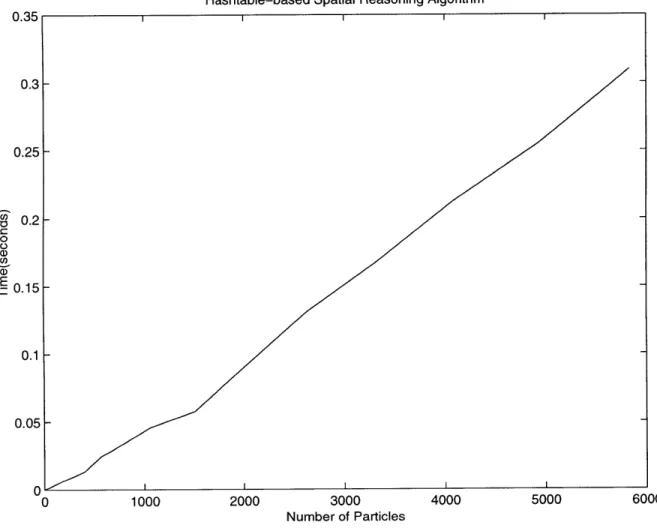
2-9 Performance Analysis of Hashtable-based Algorithms for 3D Particles for a Time Step ... ... ... ... 47

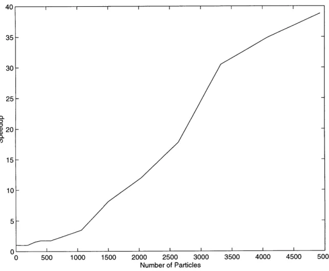
2-10 Speedup of the Spatial Hashing over Spatial Heapsort Algorithm . . . 48

3-1 Superquadrics with varying exponents . ... . 53

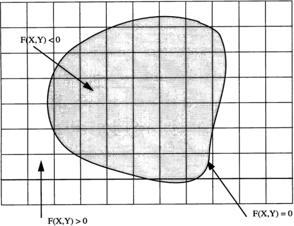
3-2 Inside-Outside Property of Implicit Function . ... 55

3-3 DFR Contact Test ... ... . 56

3-4 Discrete Function Representation [From [37]] (A) Traversal of Vertices (B) Physical To Address Space Mapping (C) Projection of B to A (C) Projection of Reduced A to B . ... . . . . 58

3-5 DFR 3D Algorithmic Description [From [37]] . . . . 3-6 DFR Contact Detection Process . . . .... 3-7 Performance Analysis of DFR Algorithms . . . . . 3-8 Runge-Kutta-Nystrom Numerical Integration Steps 3-9 Contact Resolution Details . . . . . . .. 3-10 Contact Table Description . . . . . . . ..

4-1 Software Framework of Modeling Environment . . . 4-2 Open Inventor Architecture . . . .. 4-3 Example of a Scene Graph . . . . . . .... 4-4 A Sample Open Inventor Scene . . . . 4-5 Example of a VRML Scene ...

5-1 Parallel Computer Architecture . . . .. 5-2 Communication Networks ...

5-3 Message Passing Programming Model . . . . 5-4 Multithreaded Programming Model . . . .

5-5 Parallel Hashtable-based Parallel Algorithm . . . . 5-6 Parallel Efficiency of Parallel Algorithm . . . . 5-7 System Architecture of Distributed Modeling Envir

6-1 Dynamic Impact Simulation Snapshot 1 . . . . 6-2 Dynamic Impact Simulation Snapshot 2 . . . . 6-3 Dynamic Impact Simulation Snapshot 3 . . . . 6-4 Contact Damping Simulation Example 1 . . . . 6-5 Contact Damping Simulation Example 2 . . . . 6-6 Contact Damping Simulation Example 3 . . . . 6-7 Sandglass Simulation . . ...

6-8 Embankment Simulation . . . .. 6-9 Wave Propagation Simulation . . . .... 6-10 Particles Rolling on the Slope ...

. . . . . . . 59 .. . . . 60 . . . . . . . 61 . . . . . 63 . . . . . . . . 65 . . . . . 67 . . . . . 72 . . . . . . . 73 . . . . . . . . 76 . . . . . 78 . . . .. . 81 . . . . . 9 1 . . . . . . . 93 . . . . . 94 . . . . . 97 . . . . . . . . 102 . . . . . 103 )nment ... 104 . . . . . 107 . . . . . . 108 . . . . . . . 109 . . . . . . . 111 . . . . . . . 112 . . . . . . . . 113 . . . . . . . . 114 . . . . . . . 115 . . . . . . . 117 . . . . . . . 118

6-11 Fracture of a Fixed-end Beam . ... . . . 119

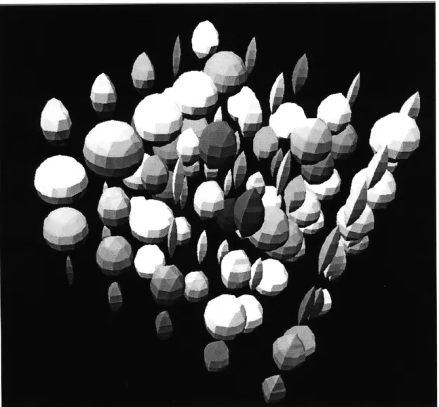
6-12 DFR Packing Simulation . ... . . . .. 121

List of Tables

2.1 Index Tables Before Heapsort . ... . . . . . 32 2.2 Index Tables Following Heapsort . ... . . . 33

Chapter 1

Introduction

1.1

Motivation

Recently, the discrete element method (DEM) has emerged as an attractive approach for scientists and engineers to study materials and systems at the granular and par-ticulate level where the traditional numerical methods have been unsuccessful. For example, the fundamental aspects of the behavior of granular materials can not be accurately simulated using these traditional methods because of the assumption of material continuity inherent in their derivation.

To set up a physical experiment to study materials at the granular level is a difficult task. Using the discrete element techniques, reseachers can investigate the behavior of materials at the microscopic level. In order to analyze systems at the particle level, the simulation has to be able to deal with thousands or even millions of objects. Scientists have attempted to model how materials crack at the atomic level by using millions of particles and parallel computation [1]. There are several important research issues that must be addressed in developing a simulation capable of analyzing large number of particles, especially if the particles have complex geometric shape and internal state. This thesis identifies and address the computational issues of building a DEM simulation that can operate on today's workstation.

1.1.1

Problem Description

The number of particles which can be analyzed is limited by the available computing resources. As a result, most discrete element simulations have focused on small scale problem with hundreds or thousands of particles, often idealized in two dimensions. The goal of this thesis is to develop efficient approaches to reducing the computational complexity of the discrete element algorithms. Our goal is to be able to handle

approximately one million bodies in a full three dimensional simulation.

It is generally acknowledged that the collision detection is the major computa-tional bottleneck in DEM simulations. In order to facilitate the DEM simulation, we seek highly efficient collision detection algorithms to reduce the required computing time to an acceptable level. We will show a simple example to illustrate the need for efficient methods of contact detection.

1.1.2

Example

Suppose that we have a system composed of M objects and each object is represented with N surface points in 3D. If there is no efficient algorithm involved, then the computational complexity of correctly detecting all the geometric overlaps between particles is given by Equation [1.1].

Computational Complexity of all - to - all check = O(M 2N2) (1.1)

For instance, if we simulate a system with 10,000 particles, and each particle is described by 1,000 surface points in 3D and we have a fast computer which can perform an operation in 10-6 seconds, then, it will take 3 years to perform the contact detection of a single timestep as shown in Equation [1.2]. It is obvious that this kind of approach is not acceptable and we must invent more efficient algorithms.

The spatial heapsort algorithm was developed to enhance the performance from O(M2) to O(MlogM) [37]. Also, the computational cost of checking the intersection of a pair of particles is varied depending on the data structure chosen to represent the object geometry. The typical geometric representation schemes, such as polygon or surface patches, commonly used in computer graphics research, are not optimal for DEM because of their inefficiency in contact detection. Instead, we use an alternative called the discrete function representation (DFR) [37] which gives O(N) performance, where N is the number of surface points. By combining the spatial heapsort algorithm and DFR, we can reduce the computing time to about 2 minutes, as shown in Equation

[1.3].

(MlogM)(N)/(time of operation) = 132 seconds (1.3)

In this thesis, a hashtable-based spatial reasoning algorithm which demonstrates

O(M) performance is developed and implemented, which further reduce the

com-puting time for contact detection. Using the same example described above, the computing time is reduced to only 10 seconds for a single step, as shown in Equation

[1.4].

MN/(time of operation) = 10 seconds (1.4)

From the above discussion, it is apparent that for large-scale problems comprising thousands of three dimensional particles, efficient contact detection algorithms are required.

1.2

Thesis Objectives

This thesis develops a distributed computing environment for multibody physics sim-ulation based on the discrete element method. It includes a set of algorithms that

significantly reduce the computational time required in DEM simulation as well as some auxiliary functionalities, such as visualization, to provide a complete simulation environment.

The following issues are addressed in this thesis, which are central to the research of discrete element methods, especially from a computational perspective.

* The implementation of an object representation scheme to model 3D objects with arbitrary geometric shape. The discrete function representation (DFR) is a high-performance scheme particularly desirable for contact resolution.

* The development of an efficient hashtable-based three-dimensional contact de-tection algorithm, which demonstrates O(M) performance, where M is the num-ber of particles in the system. This algorithm is restricted to bodies of similar size. However, this restriction can be removed if large objects are divided into sub-regions.

* The enhancement of the original sequential algorithm to perform contact detec-tion in a distributed and parallel fashion. In order to surpass the computadetec-tional barrier associated with large-scale DEM problem, implementing a the parallel processing strategy has proved to be an effective approach.

* The software framework for the simulation environment. Object-oriented tech-nology has been applied in designing the software. It provides a highly organized structure, particularly in terms of implementation and maintanence of the soft-ware.

The principal objective of this thesis is to develop a high-performance simulation environment and computational framework based on discrete element methods so that the behavior of granular materials at the microscopic level can be investigated with the minimum computing resources.

1.3

Discrete Element Method

Until recently, continuum models of materials have dominated the analysis of their behavior. Nevertheless, a number of numerical methods which start at the microscopic level have gained attention recently. These technologies include discrete element, cellular automata, lattice gas, molecular dynamics, and percolation models. They offer a complimentary view of the physics of material behavior to the traditional

techniques, such as the finite element method.

Conventionally, engineers attempt to formalize their model by deriving govern-ing differential equations to describe or idealize the behavior of the material. The assumption that the material is a continuum involves an averaging of parameters, such as density, over space and is based on the concept of a representative elementary volume (REV). This leads to a governing differential equation which includes a con-stitutive relationship defining the response of the material to external physical loads. To fully specify the model we also need to define the initial and boundary conditions so that we can derive a solution in terms of space and time.

However, this kind of "top-down" approach of treating the material as a contin-uum described by a set of governing differential equations is not necessarily sufficient to explain the behavior of granular materials. Alternatively, the "bottom-up" ap-proach that views the material as composed of distinct bodies, provides a solution for this kind of problems. As long as we can ensure that the microscopic behavior of the material is correctly described, it is rational to conclude that the emergent macroscopic behavior exhibited in the DEM simulation is also correct.

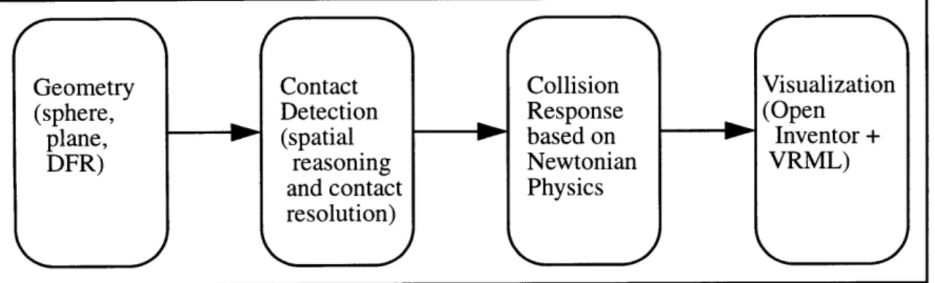
A DEM analysis can be decomposed into four computational modules described as follows:

* Geometry

Specify the object geometry, boundary conditions, and physical environment. It provides support for the generation and representation of a general class of

3D objects.

* Contact Detection

Automatically identify the object pairs which overlap with each other. It pro-vides a mechanism to automate contact detection between the objects.

* Physics

Calculate forces and integrate the motion to update the position of objects.

* Visualization and Data Analysis

Show the animation results of the analysis. Provides support for user interaction with the simulation and incorporate channels for visualization and temporal characterization of multibody simulations. Output the state of each object with time.

These items encapsulate the components of an DEM analysis pipeline which is represented in Figure [1-1]. According to Williams and Pentland [53], the major characteristics of discrete element methods can be summarized as follows:

* Simulates large displacements and rotations of disjoint bodies.

* Automatically identifies the occurence of contact between pairs of objects during the simulation process. This process is known as contact detection.

In Figure [1-2], we list the potential applications of DEM [23]. Generally, the DEM provides a complimentary numerical analysis approach to traditional methods, such as finite difference and finite element analysis.

1.4

Computational Requirements in DEM

The DEM simulation is a highly computational intensive procedure. Without efficient numerical algorithms, the entire process can be too expensive to tackle on today's

Geometry Contact Collision Visualization

(sphere, Detection Response (Open

plane, (spatial based on Inventor +

DFR) reasoning Newtonian VRML)

and contact Physics resolution)

Figure 1-1: DEM analysis pipeline

computers. To make the DEM a practical tool for engineers, from the computational persepctive, the following important requirements need to be satisfied.

1.4.1

Object Representation Requirements

In the DEM simulation environment, since all physical entities are represented by discrete objects, it is essential to provide a compact and versatile object represen-tation scheme that allows the user to define arbitrary geometric shapes of bodies. In computer graphics and computational geometry research, there are many geome-try representation methods, such as, polygonal models, constructive solid geomegeome-try, implicit surface, and parametric surfaces, that have been proposed for different appli-cations [28, 29, 34, 31]. However, the polygon-based representation is not suitable for DEM simulation because of its inefficiency in contact detection. In DEM, the object representation scheme should not only be able to describe the geometry accurately, but also needs to be helpful in collision detection.

* Offshore platforms and vessels in sea ice

- Iceberg-bottom founded structure interaction

- Icebreaker and tanker interaction with sea ice

- Seabed scouring by ice features and impact on pipeline stability

- Arching and flow studies of ice in seaways, platforms and bridge legs

- Explosive fracture of sea ice

* Behavior of soils, rocks, and granular materials

- Macroscopic constitutive behavior from microscopic granular structure

- Rock pit slope stability behavior

- Underground structure stability in jointed rocks

- Study of earthquake mechanisms and plate tectonics

- Liquification under dynamic loading

* Impact and explosive dynamics

- Automobile crash simulation

- Blast survivability studies

* Mechanical behavior

- Metal forming

- Interaction of machinery components

- Analysis of linkages and chains

- Vibration control and feedback studies

- Fracture mechanics

1.4.2 Contact Detection Requirements

Profiling the computational time in each phase of DEM simulation indicates that collision detection is the major computational bottleneck. As we saw in the previous example in Section 1.1.2, it is important to efficiently perform contact detection.

In addtion to the DEM, other application programs, such as CAD and analysis, of-ten require automated reasoning about the spatial geometry of objects. For example, numerical analysis, computer animations of physically based simulation, CAD-CAM systems, path planning and control applications in robotics all require the determi-nation and examidetermi-nation of multi-body interactions, [52, 55, 45, 41, 46, 18, 35, 39].

1.4.3

Contact Resolution Requirements

In order to simulate collision between bodies it is necessary to apply forces between the objects at the in contact surface. The collision response can be achieved in various ways and several algorithms have been proposed for different applications [35, 54, 4]. In this case we choose to use a Penalty Function formulation [37]. The contact resolution problem is concerned with computing the equal and opposite impulses that should be applied to the colliding objects, based on Newtonian mechanics. For particles with complex geometric shape, it is required to calculate the parameters, such as the mass, the location of center of mass, moments and products of inertia relative to the center of mass, etc. The volume integration scheme is introduced to provide this information. Here, all physical objects in the simulation are assumed perfectly rigid, although DEM simulations with deformable bodies are possible [40]. In Chapter 3, we will describe these requirements in details.

1.4.4

User Interface and Visualization Requirements

It is essential for the simulation program to provide a user-friendly interface for the engineers to enter the data, interact with the program, interprete the output, and

visualize the results in an integrated fashion. In this thesis, a simulation description language is developed to ease the burden of input. Also, a versatile 3D visualization post-processor allows the engineers to not only graphically view the results in any direction, but also to provide a variety of color-coding schemes to highlight different physical properties or states of the object. For example, the velocity of the body can be linked to the object color.

1.5

Characteristics of the DEM3D Simulation

Sys-tem

In this section, the basic functionality and general DEM simulation procedure of running an application using the DEM3D simulation environment is introduced. In Figure [1-3], we list the sequence of completing a single DEM simulation procedure.

1.5.1

Basic Functionality

Performing a DEM simulation requires the specification of the following items.

* Geometric Representation of Objects

For example, sphere, plane, and arbitrary shape of 3D geometry.

* Constraints

Bonding, cohesion, and collision.

* Material Properties

Stiffness, damping factor, friction, and so on.

* Simulation Parameters

Timestep, gravity, resolution, and so on.

* Visualization

1.5.2

Object-Oriented Technology

The object-oriented technology has emerged as the mainstream paradigm in the pro-gramming community nowadays. Instead of dealing with data and function sepa-rately, the object-oriented modeling and design emphasizes object, which is a high-level abstraction of data together with operations on the data. In general, the object-oriented technology is characterized by the following three attributes:

* Encapsulation (abstract characterization of objects)

* Inheritance (code sharing)

* Polymorphism (run-time binding of operations to objects)

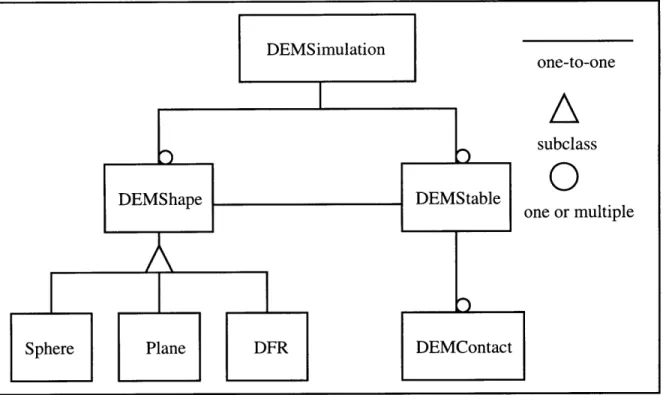
With the features mentioned above, the overall software design is more structured and maintenance becomes less complicated. The object model of the DEM3D system developed in this thesis is illustrated in Figure [1-4].

1.6

Distributed and Parallel Implementation

With the advent of powerful multiprocessor workstation and high-speed communi-cation network, it has become advantageous to migrate from the traditional sequen-tial programming model to the parallel counterpart. The hardware advancements provided by the powerful multiprocessor server and well-developed parallel program-ming software standards, such as, the message passing interface (MPI), offers a well-structured framework for integrating distributed computing resources into a simu-lation. These standards allow trasmitting and managing the data between a set of processors via a communication network. The characteristics of parallel and dis-tributed computing and details of the implementation are described in Chapter 5. In Figure [5-7], we show the current configuration of the local area network, which has a high-speed 100MBits/sec Fast Ethernet switch, an SGI server, workstation, and PC server are capable of exchanging data rapidly.

1. Specify system parameters 2. Initialize graphics subsystem 3. Create particle objects

4. Define material properties 5. Assign system parameters 6. for each timestep

(a) Run spatial reasoning algorithm to determine all candiate pair-ings

(b) for each candidate pairing

i. Perform the detailed check

ii. Apply the physics based on Newtonian mechanics (c) Increment the timestep by 1

Figure 1-3: Generic DEM Simulation Procedure

1.7

Review of Other DEM Systems

In the past few years, a wide variety of DEM systems have been implemented for various applications using different representations for the individual elements. In applications areas, such as soil mechanics, rock and ice mechanics, process engineering and granular flow, mining and blasting, and physically-based modeling and animation, some DEM systems have been designed to fit their application-specific needs. An excellent review of a variety of DEM simulation systems can be found in [37].

1.8

Thesis Outline

The major software components of a discrete element system are the object represen-tation, contact detection, and physics and visualization. Chapter 1 gives an overview

Figure 1-4: The Object Model of DEM3D system

of each component.

In Chapter 2, we deal with the spatial reasoning algorithms for contact detection. One is the spatial heapsort method, which has O(M log M) computing complexity. The other is the hashtable-based spatial reasoning algorithm, which exhibits O(M) performance.

Chapter 3 describes object representation scheme with emphasis on the discrete function representation (DFR). The superquadratic representation is introduced first to describe the rationale behind the DFR method. The incremental collision reso-lution scheme and contact table data structure are also introduced to deal with the collision response problem.

Chapter 4 covers the implementation issues of the simulation environment, in-cluding visualization graphics, such as Open Inventor graphics library and Virtual Reality Modeling Language (VRML), a matrix transform library for geometric trans-formation operations, and a simulation description language based on the Tcl/Tk toolkit. one-to-one

A

0

Chapter 5 presents the extension of the original system to a parallel version. A brief introduction to the parallel computing paradigm and programming models is given first. The Message Passing Interface (MPI) system, an emerging standard language for parallel computation, is used as the vehicle to perform the data commu-nication in the distributed simulation system. The overall parallel efficiency is shown to be satisfactory.

Several sample applications, including dynamic impact simulation, contact damp-ing, sandglass, collapse of embankment, stress wave propagation, particles rolling on

a slope, fracture of a fixed-end beam, and DFR packing are presented in Chapter 6 to demonstrate the performance and capabilities of the simulation system.

Finally in Chapter 7 conclusions about the research are summarized and prospec-tive future research directions are discussed.

Chapter 2

Algorithms for Spatial Reasoning

2.1

Introduction

As discussed in Chapter 1, the most computationally demanding process of the dis-crete element method-based simulation is the contact detection. It is estimated that contact detection occupies 85-90% of the overall computing time. As a result, we focus on this problem and propose algorithms which dramatically reduce the computational cost. In order to efficiently sort out the spatial relationship among the particles, we develop and implement two algorithms in this chapter aimed at significantly reducing the computational time.

Basically, the entire contact detection process can be subdivided into a spatial ordering phase and a contact resolution phase. During the spatial ordering phase, the contact detection algorithm has to figure out what particle pairings are possibly in contact with each other without having to exactly estimate where the contact point is. In other words, in this phase, as long as two particles are close based on some given criteria, we consider it is a candidate pair that requires further checking. Enter-ing the contact resolution phase, the algorithm computes the details on the contact geometry the and resolves the physical interaction between the contact pairings based on Newtonian mechanics.

During the spatial ordering phase of contact detection process, spatial reasoning algorithm determines which pairs of particles should be considered for the further processing in the contact resolution phase. The goal at this stage is to avoid an exhaustive brute-force check of all pairings and thereby reduce the computational cost. Once the spatial ordering of the objects is complete the algorithm identifies all the possible candidate pairs of objects which may penetrate into each other based on a criterion, such as bounding box or bounding sphere overlap. The issues of the spatial ordering phase contact detection are investigated further in this chapter. The detailed checking phase is discussed in Chapter 3.

One is the spatial heapsort scheme, named after the computing method and data structure used in this algorithm. By sorting the ordinates of the particles in each dimension, the algorithm decides which pair of particles is close enough to each other and requires further detailed check. As compared with the naive all-to-all check algorithm described in Chapter 1, this method reduces computing complexity from

O(M2) to O(MlogM) , where M is the total number of particles in the simulation system.

The other algorithm is the hashtable-based spatial reasoning scheme, have called spatial hasing, named after the data structure used in this algorithm. In the spatial hashing algorithm, the space is subdivided into a grid of cells based on the radius of the largest particle in the system and each body is assigned to a cell based on the hashing of its centroid coordinate. Independent of the particle density, this algorithm demonstrates O(M) computing complexity, where M is the number of particles in the system.

The general requirements for designing high-performance contact detection algo-rithms are as follows:

* Robustness

Robustness, in this context, means the stability of the algorithmic performance over a wide range of problems. A robust algorithm will exhibit good

perfor-mance over all cases. No matter what the composition and distribution of the particles in the system, a robust algorithm should exhibit a good performance.

* Correctness

A correct spatial reasoning algorithm should be able to identify all geometric overlaps within a given timestep. For simulation, the collision detection algo-rithm is only invoked at discrete sample times. No matter what the minimum sampling period of the collision detection system, one can choose a particle speed such that the particles entirely pass through with each other between collision checks. In our DEM simulation environment, the time step is chosen so that this cannot occur.

* Performance

In theory, the performance of a spatial reasoning algorithm is a function of the number of partilces in the system. The naive all-to-all check procedure has computational complexity O(M 2), where M is the number of particles. The

hashtable-based spatial reasoning algorithm shows a linear relationship between computing time and the number of particles. This is a significant improvement, particularly as M grows large.

* Parallelizability

A high-performance contact detection algorithm should be able to be paral-lelized without substantial data transfer overhead between processors or exces-sive extra memory requirements. In our studies, we found that there are some algorithms, for example, the hashtable-based spatial reasoning algorithm, that are highly parallelizable. This kind of algorithm always demonstrate high per-formance if the proper hardware configuration and software tools support for parallel computation are available.

The detailed theoretical analysis and empirical results of these two algorithms are given at the end of this chapter.

2.2

Spatial Sorting Algorithm

2.2.1

Introduction

There are several spatial sorting techniques which have been practically employed in different areas of application, such as the discrete element method (DEM) [52, 49, 47, 8], geometric modeling [32], computer graphics [42, 44, 25], molecular dynamics [43, 50, 21, 20, 15, 7], as well as geographical information systems (GIS) [44]. An excellent review of these sorting strategies is presented in [37].

Without examining the spatial coherence of the objects involved in a given environ-ment, an all-to-all sequence of checks for potential collision needs to be performed. For a handful of objects, this could be acceptable [22]. However, if we expect to perform the simulation for thousands of objects, the order of the computational com-plexity dominates all other considerations and methods must be sought to reduce the work involved. Several commonly applied methods to reducing the computational complexity are reviewed below:

Cellular Subdivision

The cellular subdivision method subdivides the 3D space into equal-sized cells. Each cell is given a new coordinate number based on the size of the cell. Each particle in the system is assigned to the cell which the center of its bounding box or bounding sphere belongs to.

This method can be algorithmically described as follows:

* Construct a list in all cells.

* Add all objects contained (fully or particlally) in each cell to the list.

* Check for collision of all objects within the same cell.

* Spatial distribution of the objects This static approach is suitable for prob-lems with proportionately distributed particles.

* Range of particle size If the size of the particles varies greatly, then we can only subdivide the space according to the size of the smallest particle.

* Cell resolution This is related to the particle size. The memory requirment can be extremely high if the particle size is fairly small.

In order to surpass these limitations, dynamic data structure and adaptive cell methods can be adopted to handle certain extreme cases.

Adaptive Cell Methods

Adpative cell methods aim at avoiding the space resource costs associated with the static uniform cell approach when the particles are disproportionately distributed in the simulation space.

In this approach the simulation space is discretized by cutting planes parallel to the principal Cartesian planes, x- y, y- z and z-x respectively so as to keep approx-imately the same number of particles on either side of the cutting plane. This scheme is suitable for the simulation space where particles are unevenly distributed. For the uniformly distributed case, this method will suffer from excessive data maintenance overhead in comparison with the static cellular subdivision approach.

Octree Method

The Octree method is theoretically perhaps the most elegant technique to tackle the problems of spatial coherence and resolution and the tradeoff between space and time [37]. In theory, the time required to create the octree is O(MlogM) and the time needed to search the tree is also O(MlogM). A comprehensive and complete explanation of the quadtree and octree methods can be found in [44].

The basic idea behind the Octree method is similar to the cellular subdivision method, which is to treat the simulation space as consisting of uniform-sized rectan-gular cells. However, the hierarchical tree data structure, allows us to manage only those cells which contain objects. By nature, the performance of the Octree method is heavily influenced by the distribution of the particles. Irregular distribution can generate a highly unbalanced tree which can result in the worst case of constructing and searching the tree in O(MlogM).

The octree method may not be so attractive for us because of the dynamic be-havior of the objects in DEM environment. At each timestep, the program must reconstruct the tree and search through the tree without taking advantage of the temporal coherence with the previous frame.

2.2.2 Spatial Heapsort

In this section, the spatial heapsort algorithm with running time O(MlogM) is intro-duced. There are two arrays required for each dimension of the problem domain. One is used to store the object identifiers, the other is used to rank the order of objects. The combination of these two arrays are referred to as a sorting table. The size of the array is equal to the number of particles. A typical sorting table is shown in Table

[2.1] and Table [2.2].

2.2.3 Example

In this section, we present a simple example to clarify how this spatial sorting algo-rithm works. For simplicity purpose, we start with a 2D example, and then we will show how to extend to handle 3D problems.

A collection of 2D objects with similar geometry are shown in Figure [2-1]. Each object maintains a bounding box expressed in the world coordinate system. The lower bound extents are projected onto the X and Y axes as shown in Figure [2-1]. To perform the spatial heapsort in 2D, four arrays of integers are required, two for

Y , I -, -F - , I I I i t I I I S I I I I I I I I I I I I I i I I I I I I I I I I I I I I i I I J"- - - -L J - - -- L - - - - L J - -- L J .... -- - -- - - - - I - I -

-2-,, _I7 -_ _ _~_- - -I-I II FI LL---L_ -- __ :I _I_ I-

-I I I I I I I Canonical index 1 2 3 4 5 6 7 8 9 10 11 X-dir object id 1 2 3 4 5 6 7 8 9 10 11 X-dir auxiliary 1 2 3 4 5 6 7 8 9 10 11 Y-dir object id 1 2 3 4 5 6 7 8 9 10 11 Y-dir auxiliary 1 2 3 4 5 6 7 8 9 10 11 I I [ ! 1 I

I I I

I

I

I

I

x

Table 2.1: Index Tables Before Heapsort

each dimension. The first array (sort array) initially stores the object identifiers. The second array (auxiliary array) is used to store the location of each object in the first array. Each of the first arrays is initially treated as an unsorted (implicit) binary tree, which will be sorted using the heapsort scheme. The contents of the arrays corresponding to the objects in Figure [2-1] are listed in Table [2.1]:

The next stage in the algorithm is to group objects that are candidates for colli-sion with each other. A key expedient to quickly and methodically identify candi-date pairings for collision detection is to process the sorted lists object by object in ascending order along the primary axis parallel to the simulation volume. For an

Canonical index 1 2 3 4 5 6 7 8 9 10 11 X-dir object id 6 2 3 9 1 5 10 8 4 7 11 X-dir auxiliary 5 2 3 9 6 1 10 8 4 7 11 Y-dir object id 5 3 10 6 4 9 2 11 8 1 7

Y-dir auxiliary 10 7 2 5 1 4 11 9 6 3 8

Table 2.2: Index Tables Following Heapsort

equi-dimensioned simulation volume, the X axis is chosen in the absence of any other dictating factor. Each object occurring along the axis of the chosen sorted list is se-lected. The object selected for testing is referred to as the pivot object. By processing the sorted list sequentially, candidate pairs need only be identified once as only those objects lying ahead of the pivot object need to be considered. This approach is chosen to avoid of double check between an pair of overlapped objects.

To identify the local group of objects that are candidates with the pivot object, the following steps are performed:

1. Start at the index location of the pivot object and traverse the sorted list using a binary search. Compare the largest ordinate (extent) of the pivot in the direction of the search direction/axis with the smallest ordinate of those objects lying beyond it.

2. Stop at the index location of that object which does not have a lower-bound extent less than the upper-bound extent of the search pivot.

3. Start at the index location of the search pivot in the other coordinate directions (i.e. the Y, Z axes) and traverse the sorted list using a binary search and identify the upper and lower bounds on the indices that capture all collision candidate objects in these directions.

The two steps above, obtain the lower and upper bound indices of those objects that might be in contact with the pivot object, in each of the coordinate directions.

The final stage is the detailed contact detection between pairs of objects drawn from the the intersection of the index sets. Again, the indices from the primary search direction are used to control and identify the sequence of objects examined. For each index in this list, the index of the object is found from the auxiliary index array. This index is then used to determine if the same object exists in the candidate list

of objects found along each of the secondary axis directions. If the index exists (i.e. it is an element of the intersection set of indices from all directions) a full contact detection is performed on the pair of objects.

For the example set of objects shown in Figure [2-1], using the X axis as the primary search axis, the object 4 has canonical index 9. The index bounds from the object identifier list in the X direction for objects that object 4 may be in contact with are 10 to 11 corresponding to objects {7,11}. In the secondary direction (Y axis) the index bounds from the object identifier list are 6 to 9, corresponding to objects {9,2,11,18}. The intersection of the sets of indices yields the set {11}, i.e. only a detailed contact examination of objects 4 and 11 needs to be performed.

2.2.4 Implementation

The psuedo code of the heapsort algorithm is given below.

heapsort_init(); /* initialize the data structure */ /* invoke the sorting routine in each dimension */

heapsort (X); /* X-direction */ heapsort (Y); /* Y-direction */ heapsort (Z); /* Z-direction */

map_rank (); /* generate the auxiliary array */ for each body { /* the pivot particle */

neighbours (&lx, &rx, X); /* get lower and upper bound of X */ neighbours (&ly, &ry, Y); /* get lower and upper bound of Y */ neighbours (&lz, &rz, Z); /* get lower and upper bound of Z */

/* multiplex neighbourhood indices from smaller index subset */

if (((rx - lx) >= (ry - ly))) { /* if y-list is smaller */

for (j = ly; j <= ry; j++) {

y2x = rank EX] [index [Y] [j] ;

y2z = rank[Z] [index[Y] [j]] ;

/* map Y index into X & Z indices*/

if (((y2x >= lx) && (y2x <= rx))&&((y2z >= lz)&& (y2z <= rz))){

call detailed check procedure

}

}

} else { /* if x-list is smaller */

for (j = lx; j <= rx; j++) {

/* map X index to Y index */

x2y = rank Y] [index X] [j]] ; x2z = rank[Z] [index[X] [j]];

/* IF mapped index in X & Z index ranges AND not self */

if (((x2y >= ly) && (x2y <= ry)) && ((x2z >= lz) && (x2z <= rz))) {

call detailed check procedure

}

}

}

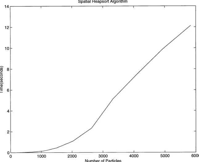
2.2.5 Performance Analysis

In theory, there are some characteristics of the heapsort algorithm [37] listed below.

* Theoretically [48], the heapsort supposedly sort an unordered collection of M objects in O(MlogM) computation time.

Spatial Heapsort Algorithm 14 12- 10-c 8-C o o E 6- 4-2 0 0 1000 2000 3000 4000 5000 6000 Number of Particles

Figure 2-2: Performance of Spatial Heapsort Algorithm for 3D Particles for a Time

* The storage requirements are O(M). No extra storage is required because the algorithm sorts in place.

* The behavior of the algorithm is stable in terms of spatial distribution of the objects to be sorted. Extreme cases will not downgrade the performance too much.

* It is straightforward to implement because no complicated data structure is required.

The empirical results of the spatial heapsort algorithm are illustrated in Figure [2-2].

2.3

Hashtable-based Spatial Reasoning Algorithm

In the following sections, a high-performance contact detection algorithm with total detection time linearly proportional to the number of particles is described in detail [36]. Furthermore, we emphasize that its performance is independent of the packing density of particles in the system.

2.3.1

Introduction

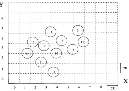
In the remainder of this section, the algorithmic description of this spatial reasoning algorithm is presented. The hashtable-based spatial reasoning algorithm is based on the assumption that each discrete element can be represented by a bounding sphere in 3D or by a circular disk in 2D. The diameter of an equivalent sphere 2R is obtained from the size of the largest discrete element in the system.

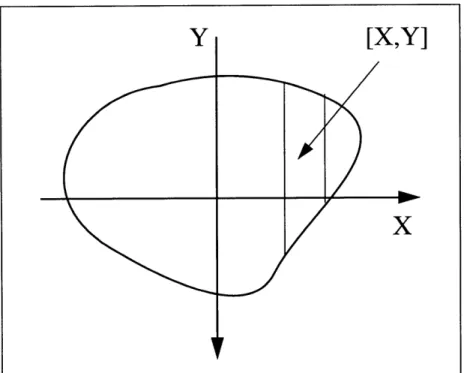
The space boundaries are defined by Xi,,Xm,ax,Ymn,Ymax, as shown in Figure

[2-3]. All particles are confined within the boundaries. The task here is to search all pairs of objects that are close enough to each other that we can say they are in contact in the spatial reasoning phase. After we pick up all the possible candidate

pairs, the detailed check for overlap will be performed by another procedure, which is described in Chapter 3.

First, the space is subdivided into identical square cells of size 2R, where R is the radius of the particle. Each particle is assigned with a unique integer identification

number from 0, 1, 2, ..., M - 1, where M is the total number of particles. Similarly,

we assign each cell an identification integer number pair (Coordx, Coordy) based on the space decomposition. The (Coordx, Coordy) pair, in this context, is the new coordinate for each cell in the system, as illustrated in Figure [2-3]. Equation 2.1 and 2.2 show how this new coordinate number is calculated.

(Coord-x) = Integer(X - X_min/2R) (2.1)

(Coord_y) = Integer(Y - Y-min/2R) (2.2)

From this criterion, we can map each object onto one and only one cell in the new coordinate system. With this new integerized coordinate, we can build a set of linked lists for each coordinate both in X and Y directions. Figure [2-4] shows the Y-direction linked list for the example in Figure [2-3]. Considering the efficient

management of memory, we exclude the use of a 2D array to represent the 2D space in our implementation. Obviously, if the range of the 2D space is large, we end up having a sparse 2D matrix, which is not an economical utilization of memory resources. The same conclusion applies to the 3D situation.

First, we traverse through the entire particle set, and give each object the Yi number. For all the objects with the same Yi, we create a linked list for this Yi number, and then insert the objects into the list sequentially, such as in Figure [2-4]. We use two integer arrays to represent this linked list. The first array YLIST contains the number of the last particle mapped to each Yi row. It is a 1D array

array of size M, where M is the total number of particles. For each particle the array

Y_LISTN stores the next particle in the singly connected list. For both array, (-1) is

used as a termination of a singly connected list. Therefore, if there is no element in a particular row, -1 is assigned to the corresponding element of the Y_LIST array. Similarly, each element in the Y_LISTN points to the next particle in the list ending with a (-1).

Example

In this section, we demonstrate a simple example to describe the rationale behind this algorithm. Starting with an example in 2D, the extension to 3D can be derived in a similar fashion.

For the example shown in Figure [2-4], there is not particle located in row 0 of the cells. Therefore, the singly connected linked list for this row, where Y = 0, would be empty. The emptiness is represented by setting the Y_LIST[O] = -1. For particle 5 mapped onto row 2, we set Y_LIST[1] = 5. Similarly, for row 4, the last particle mapped onto it is particle 10, thus Y_LIST[3] = 10. The next particle on this row is 9, thus YLISTN[10] = 9; the next particle is 6, thus Y_LISTN[9] = 6; and the last particle is 4, thus Y_LISTN[6] = 4, and Y_LISTN[4] = -1, as shown in Figure [2-4]. All Y lists are marked new at this point.

Secondly, by looping over all particles, a new Yi list is traversed and then marked as old. Each particle from this list is placed onto a corresponding ((X2, Y)) list based

on the integerized coordinate Xi. A ((Xi, Y,)) list actually contains all particles with integerized coordinate ((Xi, Y)). In addition, all singly connected lists ((Xi, Yi)) contain all particles from the list (Y) and are represented by two array of integer

numbers. The first list is a 1D list (XLIST) of size NX, where NX is the number of cells in X direction, that is, the total number of columns of cells. The second list is a 1D list (X_LISTN) of size M, where M is the total number of particles

relationship between particles.

Take the list Y3 in Figure [2-4] for example, containing particles (4,6,9,and 10). Thus the corresponding X-IST[4] = 6, X_LIST[6] = 9, X_LIST[9] = 10, and XLIST[10] = -1. In list Y3, there are no particle having an integerized

co-ordinate Coordx equal to (0,2,6, or 7), thus the singly connected lists (Xo, Y3), (X2, Y3), (X6, Y3), and (X7, Y3) are empty. Therefore, the corresponding XLIST[O],

XLIST[2], XLIST[6], and XJIST[7] are all assigned with (-1), as shown in Figure

[2-7].

Contact Detection

After constructing the data structure described above, we can proceed to perform the contact detection by checking all the particles in the neighbouring cells. Take the cell (Xi, Y) for example, we should check all the particles in cells (X,, Y), (Xi-, Yi), (X-1,Y_), (Xi, Y_), and (X+,Yjj). Starting from the (Yi=0) list, each time we select two lists (Y) and (Y+1

)

beginning to the end, we should be able to pick up all the possible contacts between particles. In other words, we do not necessarily to check all the surrounding eight cells, which will result in some duplicate pairs because of the double check. For instance,

we should only check the neighbouring cells, (X4, Y3), (X3, Y3), (X3, Y2), (X4, Y2), and (X5, Y2), for the pivotal cell (X4, Y3), as shown in Figure 2-8]. Moreover, checking

with the neighbouring cells is only performed for the non-empty cells.

Apparently in this scenario, there's no loop running over all the cells, which implies the performance of the algorithm is independent of the number of cells. Furthermore, it indicates it is also independent of the packing density of the particles.

A variety of different 3D simulation problems have been tested against the theo-retically predicted performance in Section [2.3.5].

y ---- - - -I I- I --6 I L-- J- -r- ---- -- -- ---- -5 I 1 -- I S I I 7 I X 0 1 _{I_} 2 _J i _{_ i_~r--} 5 6 i4 7 _{-_-_-__} 8 _{__----.. .I}I 2R 7 9 I I 3

Figure 2-4: Y-Direction Linked-List

t-',- # 41--' ;t I-~ -- I ~~? I I I I I I I I---I I I I I i I -I -- r I -I- I I -2 3 4 5 6 7 8 2R

Figure 2-3: Example of Hashtable-based Spatial Reasoning Algorithm

4

Y_LIST

-1

1

5

1

3

1

-1

1

4

1

2

-1

1

-1

-1

-1 -1

0 1 2 3 4 5 6 7 8 9 10

-1

1

7 8

-1

1

6

1 -1

1

9

1

-1

I11

10 -1

-1

Y_LIST_N

Figure 2-5: Data Structure of Y-Direction Linked-List

i

i

iII

6 9 10 4

X_LIST

-1

1

6 -1

1 9

1 10

1

4 -1 - I

-1

-1

-1

-1

0 1 2 3 4 5 6 7 8 9 10

-1 -1 -1 -1 I-1 I -1 I -1 I -1 I -1 I -1 -1 -1

X_LIST_N

Figure 2-7: Data Structure of X-Direction Linked-List

Sr-:---:-:---6 5 _{yI i 7 ...} I' , I I I I I I i I i i I i I I I I I i I I I I I I I I I I I I I I 1 i i I I I I I I I I I I 0 X S3 4 1--- 7 8 Fg r 2 tI I I I II I I I I I .. , IL ..J.. . . - -- ....

1__

,

2.3.2

Hashtable Data Structure

In order to reduce the amount of memory requirements, we need to develop a com-pact data structure to minimize the memory usage. Without an efficient memory management subsystem, the overall performance of the algorithm could deteriorate to an unacceptable level in practice.

In this algorithm, we use the linked-list (e.g., Y_LIST, Y_LISTN, X_LIST, X_LISTN) to store and manage the required information. The layout of the linked-list is illus-trated in Figure [2-5] and Figure [2-7].

2.3.3

Implementation

Based on the data structure described above, we now go through each step of the algorithm to explain the implementation details.

The pseudo code for this algorithm is shown below.

/* Sort objects into bins in each dimension. */

function hashspace_sort ()

{

/* 1. build the Coord_Y lists */ for each particle {

Coord_y = hash(centroid,radius); Y_LIST->insert(obj, coord_y);

}

for each particle { if(Y_LIST[i] != -1) {

/* 2. set up X_LIST lists for Coord_Y and Coord_Y-1 */ while (Y_LIST->head [i]) {