HAL Id: hal-00317445
https://hal.archives-ouvertes.fr/hal-00317445
Submitted on 1 Jan 2002
HAL is a multi-disciplinary open access
archive for the deposit and dissemination of
sci-entific research documents, whether they are
pub-lished or not. The documents may come from
teaching and research institutions in France or
abroad, or from public or private research centers.
L’archive ouverte pluridisciplinaire HAL, est
destinée au dépôt et à la diffusion de documents
scientifiques de niveau recherche, publiés ou non,
émanant des établissements d’enseignement et de
recherche français ou étrangers, des laboratoires
publics ou privés.
event on mesospheric odd nitrogen using a detailed ion
and neutral chemistry model
P. T. Verronen, E. Turunen, Th. Ulich, E. Kyrölä
To cite this version:
P. T. Verronen, E. Turunen, Th. Ulich, E. Kyrölä. Modelling the effects of the October 1989 solar
proton event on mesospheric odd nitrogen using a detailed ion and neutral chemistry model. Annales
Geophysicae, European Geosciences Union, 2002, 20 (12), pp.1967-1976. �hal-00317445�
Annales Geophysicae (2002) 20: 1967–1976 c European Geosciences Union 2002
Annales
Geophysicae
Modelling the effects of the October 1989 solar proton event on
mesospheric odd nitrogen using a detailed ion and neutral
chemistry model
P. T. Verronen1, E. Turunen2, Th. Ulich2, and E. Kyr¨ol¨a1
1Finnish Meteorological Institute, Geophysical Research Division, P.O. Box 503, 00101 Helsinki, Finland 2Sodankyl¨a Geophysical Observatory, T¨ahtel¨antie 112, 99600 Sodankyl¨a, Finland
Received: 10 October 2001 – Revised: 22 April 2002 – Accepted: 2 July 2002
Abstract. Solar proton events and electron precipitation
af-fect the concentrations of middle atmospheric constituents. Ionization caused by precipitating particles enhances the pro-duction of important minor neutral constituents, such as ni-tric oxide, through reaction chains in which ionic reactions play an important role. The Sodankyl¨a Ion Chemistry model (SIC) has been modified and extended into a detailed ion and neutral chemistry model of the mesosphere. Our steady-state model (containing 55 ion species, 8 neutral species, and sev-eral hundred chemical reactions) is used to investigate the ef-fect of the October 1989 solar proton event on odd nitrogen at altitudes between 50–90 km. The modelling results show that the NO concentration is significantly enhanced due to the proton precipitation, reaching 107–108cm−3throughout the mesosphere on the 20 October when the proton forcing was most severe. A comparison between the chemical pro-duction channels of odd nitrogen indicates that ion chemical reactions are an important factor in the total odd nitrogen production during intense ionization. The modelled elec-tron concentration for the 23 October is compared with EIS-CAT incoherent scatter radar measurements and a reasonable agreement is found.
Key words. Atmospheric composition and structure
(Mid-dle atmosphere – composition and chemistry); Ionosphere (Particle precipitation)
1 Introduction
Energetic proton precipitation as a result of solar events can significantly increase the production of odd nitrogen through impact ionization and ion chemistry (Crutzen et al., 1975; Rusch et al., 1981). During polar night conditions, when sunlight is absent, the photolysis reactions cannot destroy odd nitrogen. Because there is no other significant loss pro-cess, odd nitrogen is long lived and can be transported into
Correspondence to: P. T. Verronen (pekka.verronen@fmi.fi)
lower mesospheric and even stratospheric altitudes as well as into lower latitudes (Siskind et al., 1997; Callis and Lam-beth, 1998). If transported to the stratosphere, the extra odd nitrogen could be important to the ozone balance because it reacts with ozone in one of the catalytic reaction chains that, in addition to the pure oxygen chemistry, are important to the ozone budget.
Effects of anomalously large solar proton events, such as the August 1972 and October 1989 events, on middle atmo-sphere have been modelled in the past (Rusch et al., 1981; Jackman and Meade, 1988; Reid et al., 1991; Jackman et al., 1995). Reid et al. (1991) estimated a factor of 20 increase in NO at 60 km and a corresponding 20% loss of ozone at 40 km in the polar cap region as a result of the October 1989 solar proton event. Similar results have been published by Jack-man et al. (1995). Zadorozhny et al. (1992) have measured more than one order of magnitude increase in NO concen-tration at 50 km during the October 1989 solar proton event. In the modelling efforts mentioned above, ion chemistry has been included in the form of a single constant parameter that connects precipitation-induced ionization rate and atomic ni-trogen production. In this approach the production rate of odd nitrogen is obtained by multiplying the ionization rate by a constant, usually between 1.2 and 1.6, which is based on theoretical studies (Porter et al., 1976; Rusch et al., 1981).
In this paper we use a detailed ion and neutral chemistry model, with 55 ion species and several hundred chemical re-actions, to calculate the forcing on the mesosphere due to the October 1989 solar proton event. Our aim is to study in de-tail the production of odd nitrogen during the event. Using a coupled ion and neutral chemistry model means that it is not necessary for us to parameterise the chemical reaction chain between ionization and odd nitrogen production. Instead, it is possible to connect the measured proton flux and odd nitro-gen production by a direct calculation. Therefore, our main new input to the study of the October 1989 SPE will be the utilisation of an extensive and detailed ion chemistry scheme.
Table 1. A list of the neutral reactions that have been added to the SIC model. The sources for the reactions and rates are DeMore et al. (1994,
1992); Brasseur and Solomon (1986), and Rees (1989). Units are cm3s−1and cm6s−1for second and third order reactions, respectively. T is temperature and M is any atmospheric molecule
Reaction Reaction rate Source
O + O2+M −→ O3+M 6.0 × 10−34×(300/T )2.3 DeMore 94 O + O + M −→ O2+M 4.7 × 10−33×(300/T )2 B & S 86 O + O3 −→ O2+O2 8.0 × 10⁻¹²×e−2060/T DeMore 94 O + OH −→ O2+H 2.2 × 10⁻¹¹×e120/T DeMore 94 O + NO2 −→ NO + O2 6.5 × 10⁻¹²×e120/T DeMore 94 O + NO3 −→ NO2+O2 1.0 × 10⁻¹¹ DeMore 94 O + HO2 −→ OH + O2 3.0 × 10⁻¹¹×e200/T DeMore 94 NO + O + M −→ NO2+M 9.0 × 10−32×(300/T )1.5 DeMore 92 NO + O3 −→ NO2+O2 2.0 × 10⁻¹²×e−1400/T DeMore 94 NO + OH + M −→ HNO2+M 7.0 × 10−31×(300/T )2.6 DeMore 92 NO + HO2 −→ NO2+OH 3.7 × 10⁻¹²×e250/T DeMore 94 NO + NO3 −→ NO2+NO2 1.5 × 10⁻¹¹×e170/T DeMore 94 N + O2 −→ NO + O 1.5 × 10⁻¹¹×e−3600/T DeMore 94 N + NO −→ N2+O 2.1 × 10⁻¹¹×e100/T DeMore 94 N + NO2 −→ N2O + O 3.0 × 10⁻¹² B & S 86 H + O2+M −→ HO2+M 5.7 × 10−32×(300/T )1.6 DeMore 92 H + O3 −→ OH + O2 1.4 × 10⁻¹⁰×e−470/T DeMore 94 H + HO2 −→ OH + OH 0.9 × (8.1 × 10−11) DeMore 94 H + HO2 −→ H2+O2 0.08 × (8.1 × 10−11) DeMore 94 H + HO2 −→ H2O + O 0.02 × (8.1 × 10−11) DeMore 94 OH + O3 −→ HO2+O2 1.6 × 10⁻¹²×e−940/T DeMore 94 OH + OH −→ O + H2O 4.2 × 10⁻¹²×e−240/T DeMore 94 OH + OH + M −→ H2O2+M 6.9 × 10−31×(300/T )0.8 DeMore 92 OH + HO2 −→ H2O + O2 4.8 × 10⁻¹¹×e250/T DeMore 94 OH + H2 −→ H2O + H 5.5 × 10⁻¹²×e−2000/T DeMore 94 OH + NO2+M −→ HNO3+M 2.6 × 10−30×(300/T )3.2 DeMore 92 OH + NO3 −→ NO2+HO2 2.2 × 10⁻¹¹ DeMore 94 OH + HNO2 −→ NO2+H2O 1.8 × 10⁻¹¹×e−390/T DeMore 92 OH + HNO3 −→ NO3+H2O 7.2 × 10⁻¹⁵×e785/T B & S 86 OH + H2O2 −→ H2O + HO2 2.9 × 10⁻¹²×e−160/T DeMore 94 NO2+O3 −→ NO3+O2 1.2 × 10⁻¹³×e−2450/T DeMore 94 HO2+O3 −→ OH + 2O2 1.1 × 10⁻¹⁴×e−500/T DeMore 94 Cl + O3 −→ ClO + O2 2.9 × 10⁻¹¹×e−260/T DeMore 94 ClO + O −→ Cl + O2 3.0 × 10⁻¹¹×e70/T DeMore 94 ClO + NO −→ NO2+Cl 6.4 × 10⁻¹²×e290/T DeMore 94 O(1D) + N2 −→ O + N2 1.8 × 10⁻¹¹×e110/T DeMore 94 O(1D) + N2 −→ N2O 3.5 × 10−37×(300/T )0.6 DeMore 94 O(1D) + O2 −→ O + O2 3.2 × 10⁻¹¹×e70/T DeMore 94 O(1D) + H2O −→ OH + OH 2.2 × 10⁻¹⁰ DeMore 94 O(1D) + O3 −→ O2+O2 1.2 × 10⁻¹⁰ DeMore 94 O(1D) + O3 −→ 2O + O2 1.2 × 10⁻¹⁰ B & S 86 O(1D) + H2 −→ OH + H 1.0 × 10⁻¹⁰ DeMore 94 O(1D) + N2O −→ N2+O2 4.9 × 10⁻¹¹ DeMore 94 O(1D) + N2O −→ NO + NO 6.7 × 10⁻¹¹ DeMore 94 N(2D) + O2 −→ NO + O 5.3 × 10⁻¹² Rees 89 N(2D) + O2 −→ NO + O(1D) 5.3 × 10⁻¹² Rees 89 N(2D) + O −→ N + O 2.0 × 10⁻¹² Rees 89 N(2D) + NO −→ N2+O 7.0 × 10⁻¹¹ Rees 89
P. T. Verronen et al.: Effects of a solar proton event on mesospheric odd nitrogen 1969
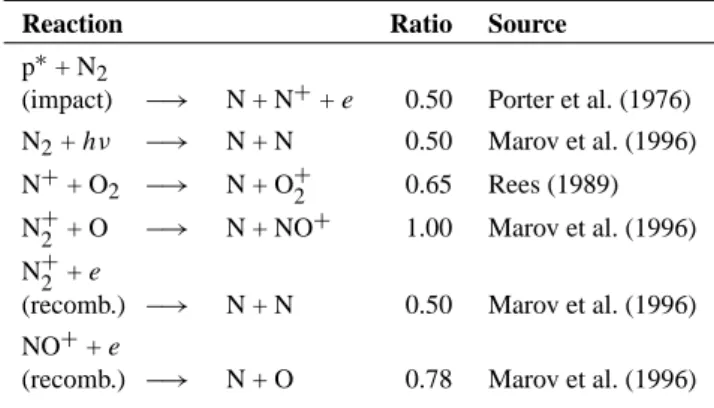
Table 2. The branching ratios for the reactions producing N(2D)
Reaction Ratio Source
p∗+ N2
(impact) −→ N + N++ e 0.50 Porter et al. (1976) N2+ hν −→ N + N 0.50 Marov et al. (1996) N++ O2 −→ N + O+2 0.65 Rees (1989)
N+2 + O −→ N + NO+ 1.00 Marov et al. (1996) N+2 + e
(recomb.) −→ N + N 0.50 Marov et al. (1996) NO++ e
(recomb.) −→ N + O 0.78 Marov et al. (1996)
2 The Sodankyl¨a Ion Chemistry model
The Sodankyl¨a Ion Chemistry (SIC) model was developed as an alternative approach to the D-region ion chemistry mod-els that connect chemical reactions to effective parameters which are set against experimental data. A detailed chemi-cal scheme, in a conceptually simple model, was built to be a tool for interpretation of D-region incoherent scatter ex-periments and cosmic radio noise absorption measurements. The SIC model was first applied by Burns et al. (1991) in a study of incoherent scatter radar measurements. Since then, the SIC model has been used in many scientific studies (Tu-runen, 1993; Rietveld et al., 1996; Ulich et al., 2000). A detailed description of the model is given by Turunen et al. (1996).
Originally the model was developed for geophysically quiet conditions. Consequently, the solar radiation (5– 135 nm) and galactic cosmic radiation (GCR) were consid-ered as ionization sources acting on five primary neutral com-ponents. Later, the model was extended to include electron and proton precipitation as ionization sources.
The SIC model can be run either in a steady-state or time-dependent mode. The model solves for the concentrations of 55 ions (36 positive, 19 negative) in the ionospheric D-region. Local chemical equilibrium can be calculated in the altitude range from 50 to 100 km with 1 km resolution. The solution for the steady state can be advanced in time, so that the response of the ion concentrations to sudden changes, such as sunrise/sunset conditions or particle events, can be studied in detail. Mathematically SIC is zero dimensional because transport processes are not included in the model.
The SIC model is based on the latest knowledge of de-tailed ion composition and the mutual reactions of the ions in the lower ionosphere; it uses background neutral atmo-spheres provided by the MSISE-90 model (Hedin, 1991), and fixed information about solar irradiance (Heroux and Hin-teregger, 1978; Torr et al., 1979). Additionally, SIC can use fixed minor neutral constituent profiles, including O, O(1D), O2(11g), O3, N, NO, NO2, NO3, N2O, N2O2, H2, H, OH,
H2O, HO2, HNO2, HNO3, HCl, Cl, ClO, CH3, CH4, CO2,
Table 3. The dissociation processes included in the SIC model
O2 + hν −→ O + O/O(1D) O3 + hν −→ O/O(1D) + O2/O2(11g) N2 + hν −→ N + N NO + hν −→ N + O NO2 + hν −→ NO + O H2O + hν −→ OH + H
and CO3, as given by e.g. Shimazaki (1984). The ionization
rate due to the galactic cosmic radiation is calculated using a parameterisation by Heaps (1978), and the ionization rate due to proton precipitation according to Reid (1961). The ionization rates due to solar UV and electron precipitation are calculated following Rees (1989).
2.1 The neutral chemistry included in the SIC model In order to investigate the effects of particle precipitation on the middle atmospheric odd nitrogen, the ion chemistry has to be coupled with relevant neutral chemistry. With the inten-tion of including all the components and reacinten-tions needed to chemically connect the ions with the odd nitrogen species, we have added 48 reactions of O, O(1D), O3, H, OH, N,
N(2D), and NO to the chemical scheme. These reactions, see Table 1, are well known and documented in standard litera-ture. The N(2D) branching ratios used are listed in Table 2. In the original model, concentrations of neutral species were fixed, so the model code has been modified to treat the eight neutrals mentioned above as unknowns.
In addition to photoionization, the photodissociation pro-cesses of N2, O2, O3, H2O, NO, and NO2have been included
in the model (see Table 3). In order to do this, the wavelength range of solar radiation was extended from the original ion-ization region of 5–135 nm and now includes also the region between 135–422 nm. The sources of absorption cross sec-tions and solar flux data are listed in Table 4. Because of a complex overlap of the O2and NO absorption bands, the
NO dissociation rate is calculated using opacity distribution functions (Minschwaner and Siskind, 1993). The N2
dissoci-ation rate is calculated according to Rees (1989). The quan-tum yield of O3dissociation between O + O2 and O(1D) +
O2(11g) around 310 nm as well as the NO2quantum yield
are considered according to DeMore et al. (1992). 2.2 Calculating the forcing due to precipitating protons There are several methods that can be used to calculate the energy input of protons and the resulting ionization rate in the atmosphere. Decker et al. (1996) have presented a compar-ison of three different modelling approaches: Monte Carlo, linear transport, and continuously slowing-down approxima-tion. They found an excellent agreement between the three methods except for the cases where protons had penetrated
Table 4. The sources for the absorption cross sections/dissociation
efficiencies and solar flux data
Wavelength Source
Solar flux 135.0–175.0 nm (Shimazaki, 1984) 175.0– 422.5 nm (WMO, 1985) O2abs. 135.0–175.0 nm (Shimazaki, 1984) 175.0–422.5 nm (WMO, 1985) O3abs. 135.0–175.0 nm (Shimazaki, 1984) 175.4–422.5 nm (WMO, 1985) N2abs. 65.0–102.6 nm (Rees, 1989) NO abs. 181.6–192.5 nm (Minschwaner and Siskind, 1993) NO2abs. 135.0–175.0 nm (Shimazaki, 1984) 202.0–422.5 nm (DeMore et al., 1992) H2O abs. 175.5–189.3 nm (DeMore et al., 1992)
Table 5. Photochemical time constants at noon (Shimazaki, 1984)
Constituent 50 km 80 km 100 km
O 10 s 3.5 h 116 d
O3 2 min 1 min 1 min
N 4.6 s 5 h 4.5 d
NO 14 min 18 h 2 d
NO2 10 s 3 s 1.5 s
H 0.1 s 44 min 12 d
OH 3.2 s 0.7 s 0.3 s
Table 6. Characteristic transport lifetimes (Brasseur and Solomon,
1986) Transport type 50 km 80 km 100 km Zonal ( ¯u) 5 h 18 h 42 h Meridional ( ¯v) 370 h 76 h 220 h Vertical ( ¯w) 890 h 890 h 570 h Diffusion 370 h 76 h 34 h
so deep that their fluxes were significantly modified, which happens well below the bulk ionization region. However, the effects of magnetic mirroring and lateral spreading of H+/H flux were turned off in the Monte Carlo calculations because the other two methods do not take these effects into account. Our current calculation is based on the energy-range mea-surements in standard air for protons by Bethe and Ashkin (1953). We also require a proton spectrum and a neutral at-mosphere in order to calculate the ionization rate. First we calculate the deposition rate of energy at each altitude, using a calculation algorithm originally presented by Reid (1961).
18 19 20 21 22 23 24 25 26 27 28 29 10−2 10−1 100 101 102 103 104 105 106
Day in October 1989 (numbers at 00:00 UT)
Counts [cm − 2 s − 1 sr − 1]
Fig. 1. Integrated proton fluxes for late October 1989 (obtained
from the World Wide Web server for the NOAA National Geo-physical Data Center), showing three-hour averages of the seven energy channels of the GOES satellite proton measurements. From top curve down the channels are: >1, >5, >10, >30, >50, >60, and >100 MeV.
Next we divide the deposited energy by the average energy loss per ion pair formation, taken to be 36 eV (see e.g. Rees, 1989, p. 40), to get the total ionization rate. The total ioniza-tion rate is then divided between the three major constituents (i.e. N2, O2, and O) according to their relative
concentra-tions and cross secconcentra-tions (Rees, 1982). Finally, we further divide the ionization rates of individual constituents between the ionization and dissociative ionization processes using the branching ratios given by Jones (1974) to obtain the produc-tion/loss rates for the individual ions and neutrals.
Protons can undergo charge-exchange reactions with the neutral molecules. However, to reach the atmospheric al-titude region between 100 and 50 km a proton must pos-sess an initial energy between ∼ 100 keV and ∼ 30 MeV. At these energies the charge-exchange reactions are not impor-tant. Further, because of the high energy of these protons their stopping power is due to ionising collisions only (Rees, 1982). Therefore, we have ignored the direct dissociation by protons. Our calculations do not include dissociation by secondary electrons. Recently, Solomon (2001) has studied ionization by secondary electrons during proton aurora at al-titudes above 80 km. He showed that the secondary electrons become progressively more important as the primary proton energy increases. The secondary electrons are an important factor in odd nitrogen production because they dissociate N2.
We will estimate the error due to exclusion of secondary elec-trons in Sect. 5.
3 Modelling the October 1989 solar proton event
In 1989, at the peak of solar maximum, there were several large solar proton events (SPE), e.g. in August, October, and
P. T. Verronen et al.: Effects of a solar proton event on mesospheric odd nitrogen 1971 100 105 50 55 60 65 70 75 80 85 90 cm−3 s−1 Altitude [km] Ionization rate 100 102 104 106 50 55 60 65 70 75 80 85 90 cm−3 Electron concentration 105 1010 50 55 60 65 70 75 80 85 90 cm−3 NO concentration
Fig. 2. The modelled ionization rate, electron concentration, and NO concentration profiles during the October 1989 SPE. Solid lines are for
the 18, dashed lines for the 20 and dash-dot lines for the 23 October.
November. In this work we model the proton event that started on 19 October 1989, had peaks on the 20, 23, and 25 October, and then decayed away. This particular SPE is one of the biggest proton events to date and it provided an extreme forcing on the middle atmosphere. Therefore, it is a good choice for a maximum effect study. The EISCAT inco-herent scatter radar was operated during the event, so that we are able to compare ground-based measurements of electron concentration with our modelling results. This was another reason for choosing this particular event.
The proton flux data from the GOES-7 satellite mea-surements for the October 1989 SPE, see Fig. 1, were ob-tained from the World Wide Web server for the NOAA Na-tional Geophysical Data Center at www.ndgc.noaa.gov/stp/ stp.html. The GOES measurements were converted to dif-ferential proton flux for 600 keV–2000 MeV range assuming that the flux can be described by the exponential rigidity re-lation (Freier and Webber, 1963). Because of the high mag-netic latitude of our calculation point (66.46◦N), virtually
all protons are able to enter the atmosphere (see e.g. Harg-reaves, 1992, p. 358). Therefore, the proton spectra at the top of the atmosphere are assumed to be the same as those measured by GOES at the geosynchronous altitude. In near-Earth space protons are found to be travelling in all directions (see e.g. Hargreaves, 1992, p. 354). For this reason, we have assumed that the angular distribution of protons is isotropic over the upper hemisphere, i.e. when calculating the ioniza-tion by protons at each altitude point, we assume that the protons can enter, if possessing enough energy, from any di-rection with pitch angle less than 90◦. Neither magnetic mir-roring effects nor further pitch angle limits were considered. For each day between the 18 and 28 October, we calcu-lated the MSISE-90 temperature and neutral concentration
profiles at 12:00 UT over Tromsø (69.59◦N, 19.23◦E). The
minor profiles that are not provided by the MSISE-90 model were taken from Shimazaki (1984). We then calculated the corresponding production and loss rates of individual ions and neutrals due to photoionization and photodissociation. We also calculated an average proton flux between 12:00 and 15:00 UT and the corresponding ion production rates due to proton penetration. Using these production rates we then calculated the steady-state concentrations for ions and se-lected neutrals taking into account the production and loss in ion/neutral chemical reactions.
During daytime, i.e. when solar radiation is present, and at mesospheric altitudes it is reasonable to assume a steady-state condition for the ions and most of the modelled neu-tral constituents because their chemical time constants (see Table 5) are shorter than the solar-illuminated period of the day, which is roughly 8–10 h for our calculation points. NO is the one exception with a chemical time constant of 18 h at 80 km. Therefore, our results for NO actually compare the production environment from day to day showing the local forcing on NO, i.e. a state that would eventually be reached if the conditions would remain the same.
We are ignoring transport effects in this study. The char-acteristic transport lifetimes are generally much greater than the photochemical time constants (Table 6). In zonal direc-tion this is not the case at 50 km altitude. However, in the case of solar proton events (also known as polar cap absorp-tion or PCA events), unlike the case of highly localised high energy electron precipitation, the effects cover the whole po-lar cap area above a certain magnetic latitude (Hargreaves, 1992). Hence, we assume that we have similar particle forc-ing conditions in the zonal regions surroundforc-ing our calcula-tion spot. Further, the general meridional wind direccalcula-tion on
0 0.1 0.2 0.3 0.4 0.5 0.6 50 60 70 80 90 Altitude [km] 0 0.1 0.2 0.3 0.4 0.5 0.6 50 60 70 80 90 Altitude [km] 0 0.1 0.2 0.3 0.4 0.5 0.6 50 60 70 80 90 N/I number Altitude [km]
Fig. 3. The N/I number, i.e. the number of odd nitrogen species
(N(4S), N(2D) and NO) created per ion pair produced by proton impact. From the top downwards the panels are for the 20, 23, and 25 October 1989. The total number is shown with the bold solid line. The dash-dot, dashed and solid lines show the contributions by dissociative ionization, ionic production of atomic nitrogen and ionic production of NO, respectively. The contribution of secondary electrons is not taken into account.
our calculations spot (69.59◦N, winter hemisphere) is from north to south, thus the wind is bringing in material from the affected polar cap area. Therefore, we assume that horizon-tal transport does not significantly affect our results in time scales of hours.
It should be noted that our calculations extend up to 90 km. We are showing all the results to get a larger picture, but one should remember that the steady-state approach gets progres-sively more questionable above 80 km when calculating NO concentrations.
4 Results
Figure 2 shows the variations of the ionization rate, electron concentration and NO concentration during the SPE. The electron and NO variations follow the ionization rate vari-ations. On the 20 October, when the proton flux peaks, we find that the ionization rate can be 7.9 × 10⁴times, the elec-tron concentration 430 times, and the NO concentration 160 times as large as the background values on the 18 October.
30 40 50 60 70 80 90 100 110 50 55 60 65 70 75 80 85 90
Portion of ionic reactions in odd nitrogen production [%]
Altitude [km]
Fig. 4. The portion of ions in N(4S), N(2D), NO and total odd
nitrogen production represented by dash-dot, dashed, solid and bold solid lines, respectively. These curves are for the 23 October 1989. The contribution of secondary electrons is not taken into account.
103 104 105 50 55 60 65 70 75 80 85 90 95 100
Raw electron concentration [cm−3]
Altitude [km]
Fig. 5. The electron concentration profiles for the 23 October 1989
as modelled by SIC (the dashed line) and measured by EISCAT (the solid line). The modelled curve is for 12:00 UT, while EISCAT curve is an average of the measurements made between 12:00 and 14:00 UT.
The same values for the 23 October are 1.8 × 10⁴, 160, and 45, respectively. For both cases the increase of ionization peaks at 50 km and the increase of electron concentration at 60 km. The increase of NO concentration peaks at 78 and 79 km on 20 and 23 October, respectively. The extreme en-hancements on the 20 October are caused by a sharp peak of the proton flux, located between 12:00 and 15:00 UT (Fig. 1). For NO, smaller changes were predicted by Reid et al. (1991), who used a 2-D time-dependent model to study the 1989 SPE and obtained the largest NO increases, up to a factor of 20, in the end of October between 60 and 80 km.
P. T. Verronen et al.: Effects of a solar proton event on mesospheric odd nitrogen 1973
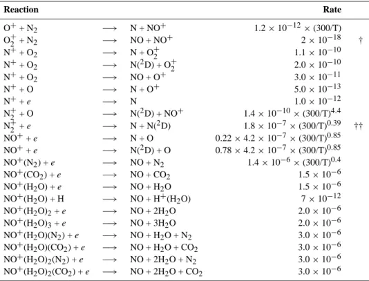
Table 7. The ionic reactions producing odd nitrogen. The sources of the reaction rates are listed by Turunen et al. (1996), except for † and
†† which are taken from Matsuoka et al. (1981) and Rees (1989), respectively
Reaction Rate O++ N2 −→ N + NO+ 1.2 × 10−12×(300/T) O+2 + N2 −→ NO + NO+ 2 × 10⁻¹⁸ † N++ O2 −→ N + O+2 1.1 × 10⁻¹⁰ N++ O2 −→ N(2D) + O+2 2.0 × 10⁻¹⁰ N++ O2 −→ NO + O+ 3.0 × 10⁻¹¹ N++ O −→ N + O+ 5.0 × 10⁻¹³ N++ e −→ N 1.0 × 10⁻¹² N+2 + O −→ N(2D) + NO+ 1.4 × 10−10×(300/T)4.4 N+2 + e −→ N + N(2D) 1.8 × 10−7×(300/T)0.39 †† NO++ e −→ N + O 0.22 × 4.2 × 10−7×(300/T)0.85 NO++ e −→ N(2D) + O 0.78 × 4.2 × 10−7×(300/T)0.85 NO+(N2) + e −→ NO + N2 1.4 × 10−6×(300/T)0.4 NO+(CO2) + e −→ NO + CO2 1.5 × 10⁻⁶ NO+(H2O) + e −→ NO + H2O 1.5 × 10⁻⁶ NO+(H2O) + H −→ NO + H+(H2O) 7 × 10⁻¹² NO+(H2O)2+ e −→ NO + 2H2O 2.0 × 10⁻⁶ NO+(H2O)3+ e −→ NO + 3H2O 2.0 × 10⁻⁶ NO+(H2O)(N2) + e −→ NO + H2O + N2 3.0 × 10⁻⁶ NO+(H2O)(CO2) + e −→ NO + H2O + CO2 3.0 × 10⁻⁶ NO+(H2O)2(N2) + e −→ NO + 2H2O + N2 3.0 × 10⁻⁶ NO+(H2O)2(CO2) + e −→ NO + 2H2O + CO2 3.0 × 10⁻⁶
Zadorozhny et al. (1992) made a rocket measurement on the 23 October 05:00 UT in the southern part of Indian Ocean (geomagnetic latitude 60◦S) and reported more than one or-der of magnitude increase in the NO concentration, com-pared to measurements on the 11 and 12 October. They found the largest increases at 50 km altitude. In our calcu-lations, the absolute NO values for the 23 October vary be-tween 1.5×10⁸and 1.5×10⁶while Zadorozhny et al. (1992)
report values between ∼ 2×10⁹and ∼ 2×10⁸. Therefore, the larger change in our calculations is not due to larger values during the event but rather because of smaller reference val-ues. The main reason for the smaller reference values is the fact that our calculations do not take into account the precipi-tation history before the 18 October, while the measurements by Zadorozhny et al. (1992) are affected by earlier particle events.
Figure 3 shows the N/I number, i.e. the number of odd ni-trogen species (N(4S), N(2D) and NO) produced per each ion pair, on the 20, 23 and 25 October. The altitude profiles show similar behaviour, a variation between 0.31 and 0.51. The-oretical calculations (Porter et al., 1976; Rusch et al., 1981) predict that 1.2–1.6 nitrogen atoms are produced per each ion pair. However, these are not directly comparable with our results because of different production mechanisms. Porter et al. (1976) included dissociative ionization by protons and dissociation by secondary electrons, Rusch et al. (1981) in-cluded the same ones as Porter et al. (1976) and also chemical production from N+and O+while our number includes
dis-sociative ionization by protons and production from ionic re-actions but neglects N2dissociation by secondary electrons.
Figure 3 shows that under the forcing of energetic proton precipitation the ionic reactions produce a significant amount of odd nitrogen in the form of atomic nitrogen and NO. Ta-ble 7 lists the ionic reactions producing odd nitrogen and Fig. 4 shows the portion of the ions in the odd nitrogen pro-duction. On the 23 October, 39%–63% of the total odd ni-trogen production is due to ionic reactions (note that we are neglecting the production by secondary electrons). The rest is produced by dissociative ionization of N2 due to proton
impact, N2photodissociation (negligible in the mesosphere)
and the reaction O(1D) + N2O −→ NO + NO (in the lower
mesosphere). When calculating the ratios we have ignored the reactions between the odd nitrogen species, i.e. N(4S), N(2D), NO and NO2.
4.1 A comparison with EISCAT measurements
Figure 5 shows a comparison between the calculated electron concentration profile and EISCAT incoherent scatter radar measurements. On the 23 October 1989 the EISCAT VHF radar was operated in a special D-region mode GEN-11, which is described in detail by Pollari et al. (1989). The al-titude region normally measured is from 70 to 113 km, with 1.05 km resolution, for a vertical antenna. This time the an-tenna was tilted towards north so that the lowest measurable altitude was 50 km. However, measurements below 54 km
are not reliable because of the instrumental limitations (Col-lis and Rietveld, 1990). The EISCAT profile presented in Fig. 5 is an average of measurements done between 12:00 UT and 14:00 UT on the 23 October 1989. The solar zenith an-gle varied between 82.7 and 89.0◦, thus the measurements were sunlit. The measured and modelled profiles clearly have the same magnitude but there are also differences be-tween them. From 66 to 87 km we have good agreement with maximum difference less than 30%. Above 90 km there is a large peak in EISCAT electron concentration that our model does not predict. Between 56 and 67 km our model predicts larger electron concentrations than the measurements, so that at 60 km there are 51% more electrons in our model. The sta-tistical error in EISCAT measurements is typically less than 10%.
At the upper altitude limit we would expect the measure-ments to show higher electron concentrations than our model calculation because we are ignoring the effect of precipitat-ing electrons as an ionisprecipitat-ing factor. The shape of the EISCAT electron concentration profile between 90 and 95 km resem-bles the one measured for neutral metallic atoms at these al-titudes (Plane et al., 1999). Therefore, the electron concen-tration peak might be a result of precipitation induced ion-ization in such a layer. At lower altitudes, we would expect the measurements to show less electrons than our model be-cause in our calculations we are using all proton energy for ionization of neutral gases, thus ignoring the energy trans-fer to secondary electrons which gain in number as altitude decreases.
5 Discussion
Recent observational analyses have shown that as a result of particle precipitation events a significant amount of odd ni-trogen is created in the mesosphere and lower thermosphere (Callis and Lambeth, 1998). According to model studies a large enough part of the created odd nitrogen is transported to lower altitudes and latitudes during winter and early spring, so that it is necessary to take into account this highly variable natural source of odd nitrogen in stratospheric ozone simula-tions (Callis, 2001). First and an important step in this task is to model accurately how the ambient atmosphere responds to particle forcing, requiring consideration of particle flux degrading, ionization of neutral atmosphere and ion chem-istry. Many modelling efforts include the ion chemistry by using simple parameterisation that might not be sufficient to present the complex chemical scheme. In this work we have used a detailed ion chemistry scheme to study the response of odd nitrogen to the October 1989 solar proton event in the mesosphere. Also, we have made a comparison between our results and commonly used parameterisation of atomic nitro-gen production.
Our model calculations show that odd nitrogen is consid-erably enhanced in the mesosphere as the result of a solar proton event. During the event, when intense ionization con-ditions prevail, ionic reactions produce a significant fraction
Table 8. The maximum error estimates for the values presented
in Fig. 2 (NO, for nitric oxide), Fig. 3 (N/I, for the total num-ber), and Fig. 4 (Ionic, for the total number). The effect of uncer-tainty of N(2D) branching ratio was studied by changing the ratio of NO++e −→N(4S)/N(2D) + O from 0.78 to 0.6
Error source NO N/I Ionic
Ionization rate calculation method −35% ±3% ±2% Uncertainty of N(2D) branching ratio −15% +2% +1% Exclusion of secondary electrons
at 50 km +5% +550% −85%
Exclusion of secondary electrons
at 60 km +20% +100% −50%
Exclusion of secondary electrons
at 70 km +10% +20% −15%
of atomic nitrogen and a major fraction of nitric oxide. Thus, the production by ionic sources not only competes but over-comes the direct production by precipitating protons. This is the main result of this study and means that the modelling approach in which the ion chemistry is taken into account by connecting total ionization rate with neutral atomic nitro-gen production neglects a significant source of odd nitronitro-gen. Therefore, we conclude that ion chemistry, at least for the main ions, should be explicitly included if realistic modelling of particle effects is attempted.
We found that the number of odd nitrogen species pro-duced per ion pair is not a constant but varies with altitude. This number variation makes sense because the parameters that affect the chemical scheme, such as temperature and gas concentrations, can have large altitude dependent gra-dients. Before making any further conclusions in this mat-ter, we want to include the dissociation effects of secondary electrons in our model. However, based on Monte Carlo cal-culations for the 23 October 1989 (V. I. Shematovich and D. V. Bisikalo, private communication), we assume that the inclusion of secondary electrons affects our results only in the lower mesosphere.
A comparison between the modelled electron concentra-tion profile and EISCAT incoherent scatter radar measure-ments showed a reasonable agreement. This implies that the ion photochemistry in our model is reasonably realis-tic. It does not directly validate the modelled neutral con-centrations. In the near future we will be able to compare our modelling results with satellite measurements of meso-spheric neutral constituents. This will be a better test of our model.
We estimate that in our calculations the greatest errors are due to the exclusion of secondary electrons, the ionization rate calculation method, and the uncertainty in the N(2D) branching ratios. The exclusion of transport is not as im-portant a source of error because the transport lifetimes are relatively long and also because the prevailing wind
direc-P. T. Verronen et al.: Effects of a solar proton event on mesospheric odd nitrogen 1975 tion at the place and time of our calculation is from the polar
cap area southwards. Based on Monte Carlo calculations for the 23 October 1989 (V. I. Shematovich and D. V. Bisikalo, private communication), we can estimate the errors due the ionization rate calculation method and the exclusion of sec-ondary electrons. Our calculation gives 40–200% higher ionization rates than the Monte Carlo method. The reason for this difference might be that a part of the energy of the primary protons is transferred to the secondary electrons, which is not considered in our calculations. The Monte Carlo results show that, at least for the case of the 23 October 1989, the secondary electrons have largest effect in the lower mesosphere and below and that their significance rapidly de-creases with increasing altitude. The NO concentration can be very sensitive to the N(2D) branching ratios. For example, Barth (1992) found that a change in the ratio from 0.75 to 0.6 in recombination reaction NO++e −→N + O caused a
change of −100% in the nitric oxide concentration at 105 km. We did a series of sensitivity calculations and in Table 8 we summarise the resulting estimates of maximum error.
During the course of this work we developed the So-dankyl¨a Ion Chemistry model to an ion and neutral chemistry model of the mesosphere. The SIC model does not try to compete with multidimensional models (Siskind et al., 1997; Callis et al., 1998; Jackman et al., 1995) that are used for long-term global studies. The strength of SIC is in extensive ion chemistry through which it can provide a detailed pic-ture of short-term local perturbations. Similar extensive ion chemistry models have been used also by Kull et al. (1997) and Beig and Mitra (1997) to study lower-latitude D-region and long-term effects of greenhouse gases in the middle at-mosphere, respectively. However, as far as we know, such a detailed ion chemistry scheme has not been used to ad-dress the particle precipitation problem before. The new SIC model is not perfect. We are still missing some input that would make our calculation more realistic, such as solar X-rays and secondary electrons. Our neutral chemistry is in-complete in the sense that we have only included photoly-sis processes and chemical reactions necessary for this work. We don’t have transport in our model, a fact that restricts the realistic model calculation period.
SIC can also be used as a time-dependent model. Our near future plans include developing and using the time-dependent version of our model to study the accumulation of NO during the whole duration of a solar proton event. With the time-dependent model we will be able to study the re-sponse of the mesosphere to rapidly changing particle flux and sunrise/sunset conditions.
This work has been done as a part of the CHAMOS (CHemical Aeronomy in the Mesosphere and Ozone in the Stratosphere) study. The aim of the study is to use a large variety of satellite and ground-based measurement data to-gether with SIC model to study the effects of energetic par-ticle precipitation on the middle atmospheric NO and ozone. For more information about CHAMOS, see Verronen et al. (1999).
Acknowledgements. The work of P. T. V. was supported by the
Academy of Finland (Finnish Graduate School in Astronomy and Space Physics). EISCAT is an International Association supported by Finland (SA), France (CNRS), the Federal Republic of Ger-many (MPG), Japan (NIPR), Norway (NFR), Sweden (NFR) and the United Kingdom (PPARC).
References
Barth, C. H.: Nitric oxide in the lower thermosphere, Planet. Space Sci., 40, 315–336, 1992.
Beig, G. and Mitra, A. P.: Atmospheric and ionospheric response to trace gas perturbations through ice age to the next century in the middle atmosphere. Part II - ionization, J. Atmos. Terr. Phys., 59, 1261–1275, 1997.
Bethe, A. H. and Ashkin, J.: Passage of Radiations through Matter, vol. 1 of Experimetal Nuclear Physics, (Ed) Segre, E., pp. 166– 251, John Wiley & Sons, Inc., New York, USA, 1953.
Brasseur, G. and Solomon, S.: Aeronomy of the Middle Atmo-sphere, D. Reidel Publishing Co., Dordrecht, Holland, 1986. Burns, C. J., Turunen, E., Matveinen, H., Ranta, H., and
Harg-reaves, J. K.: Chemical modeling of the quiet summer D- and E-regions using EISCAT electron density profiles, J. Atmos. Terr. Phys., 53, 115–134, 1991.
Callis, L. B.: Stratospheric studies consider crucial question of par-ticle precipitation, EOS, 82, 297–301, 2001.
Callis, L. B. and Lambeth, J. D.: NOyformed by precipitating elec-tron events in 1991 and 1992: Descent into the stratosphere as observed by ISAMS, Geophys. Res. Lett., 25, 1875–1878, 1998. Callis, L. B., Baker, D. N., Natarajan, M., Blake, J. B., Mewaldt, R. A., Selesnick, R. S., and Cummings, J. R.: A 2-D model simulations of downward transport of NOyinto the stratosphere: Effects on the 1994 austral spring O3and NOy, Geophys. Res. Lett., 25, 1875–1878, 1998.
Collis, P. N. and Rietveld, M. T.: Mesospheric observations with the EISCAT UHF radar during polar cap absorption events: 1. electron densities and negative ions, Ann. Geophysicae, 8, 809– 824, 1990.
Crutzen, P. J., Isaksen, I. S. A., and Reid, G. C.: Solar proton events: stratospheric sources of nitric oxide, Science, 189, 457– 458, 1975.
Decker, D. T., Kozelov, B. V., Basu, B., Jasperse, J. R., and Ivanov, V. E.: Collisional degradation of the proton-H atom fluxes in the atmosphere: A comparison of theoretical techniques, J. Geophys. Res., 101, 26 947–26 960, 1996.
DeMore, W. B., Sander, S. P., Golden, D. M., Hampson, R. F., Kurylo, M. J., Howard, C. J., Ravishankara, A. R., Kolb, C. E., and Molina, M. J.: Chemical Kinetics and Photochemi-cal Data for Use in Stratospheric Modeling, JPL Publication 92-20, Jet Propulsion Laboratory, California Institute of Technology, Pasadena, USA, 1992.
DeMore, W. B., Sander, S. P., Golden, D. M., Molina, M. J., Hamp-son, R. F., Kurylo, M. J., Howard, C. J., and Ravishankara, A. R.: Chemical Kinetics and Photochemical Data for Use in Strato-spheric Modeling, JPL Publication 90-1, Jet Propulsion Labora-tory, California Institute of Technology, Pasadena, USA, 1994. Freier, P. S. and Webber, W. R.: Exponential rigidity spectrums for
solar-flare cosmic rays, J. Geophys. Res., 68, 1605–1629, 1963. Hargreaves, J. K.: The solar-terrestrial environment, Cambridge
University Press, Cambridge, UK, 1992.
Heaps, M. G.: Parameterization of the cosmic ray ion-pair produc-tion rate above 18 km, Planet. Space Sci., 26, 513–517, 1978.
Hedin, A. E.: Extension of the MSIS thermospheric model into the middle and lower atmosphere, J. Geophys. Res., 96, 1159+, 1991.
Heroux, L. and Hinteregger, H. E.: Aeronomical reference spec-trum for solar UV below 2000 ˚a, J. Geophys. Res., 83, 5305– 5308, 1978.
Jackman, C. H. and Meade, P. E.: Effect of solar proton events in 1972 and 1979 on the odd nitrogen abundance in the middle atmosphere, J. Geophys. Res., 93, 7084–7090, 1988.
Jackman, C. H., Cerniglia, M. C., Nielsen, J. E., Allen, D. J., Za-wodny, J. M., McPeters, R. D., Douglas, A. R., Rosenfield, J. E., and Hood, R. B.: Two-dimensional and three-dimensional model simulations, measurements, and interpretation of the October 1989 solar proton events on the middle atmosphere, J. Geophys. Res., 100, 11 641–11 660, 1995.
Jones, A. V.: Aurora, D. Reidel Publishing Co., Dordrecht, Holland, 1974.
Kull, A., Kopp, E., Granier, C., and Brasseur, G.: Ions and electrons of the lower-latitude D-region, J. Geophys. Res., 102, 9705– 9716, 1997.
Marov, M. Y., Shematovich, V. I., and Bisicalo, D. V.: Nonequilib-rium aeronomic processes – a kinetic approach to the mathemat-ical modeling, Space Science Reviews, 76, 1–204, 1996. Matsuoka, S., Nakamura, H., and Tamura, T.: Ion-molecule
reac-tions of N+3, N+4, O+2, and NO+2 in nitrogen containing traces of oxygen, J. Chem. Phys., 75, 681–689, 1981.
Minschwaner, K. and Siskind, D. E.: A new calculation of nitric oxide photolysis in the stratosphere, mesosphere, and lower ther-mosphere, J. Geophys. Res., 98, 20 401–20 412, 1993.
Plane, J. M. C., Cox, R. M., and Rollason, R. J.: Metallic layers in the mesopause and lower thermosphere region, Adv. Space Res., 24, 1559–1570, 1999.
Pollari, P., Huuskonen, A., Turunen, E., and Turunen, T.: Range ambiguity effects in a phase coded D-region incoherent scatter radar experiment, J. Atmos. Terr. Phys., 51, 937–945, 1989. Porter, H. S., Jackman, C. H., and Green, A. E. S.: Efficiencies for
production of atomic nitrogen and oxygen by relativistic proton impact in air, J. Chem. Phys., 65, 154–167, 1976.
Rees, M. H.: On the interaction of auroral protons with the Earth’s atmosphere, Planet. Space Sci., 30, 463–472, 1982.
Rees, M. H.: Physics and chemistry of the upper atmosphere, Cam-bridge University Press, CamCam-bridge, UK, 1989.
Reid, G. C.: A study of the enhanced ionization produced by solar protons during a polar cap absorbtion event, J. Geophys. Res., 66, 4071–4085, 1961.
Reid, G. C., Solomon, S., and Garcia, R. R.: Response of the
mid-dle atmosphere to the solar proton events of August–December, 1989, Geophys. Res. Lett., 18, 1019–1022, 1991.
Rietveld, M. T., Turunen, E., Matveinen, H., Goncharov, N. P., and Pollari, P.: Artificial periodic irregularities in the auroral iono-sphere, Ann. Geophysicae, 14, 1437–1453, 1996.
Rusch, D. W., G´erard, J.-C., Solomon, S., Crutzen, P. J., and Reid, G. C.: The effect of particle precipitation events on the neutral and ion chemistry of the middle atmosphere, Planet. Space Sci., 29, 767–774, 1981.
Shimazaki, T.: Minor Constituents in the Middle Atmosphere (De-velopments in Earth and Planetary Physics, No 6), D. Reidel Publishing Co., Dordrecht, Holland, 1984.
Siskind, D. E., Bacmeister, J. T., Summers, M. E., and Russell, J. M.: Two-dimensional model calculations of nitric oxide trans-port in the middle atmosphere and comparison with Halogen Oc-cultation Experiment data, J. Geophys. Res., 102, 3527–3545, 1997.
Solomon, S. C.: Auroral particle transport using Monte Carlo and hybrid methods, J. Geophys. Res., 106, 107–116, 2001. Torr, M. A., Torr, D. G., and Ong, R. A.: Ionization frequencies for
major thermospheric constituents as a function of solar cycle 21, Geophys. Res. Lett., 6, 771–774, 1979.
Turunen, E.: EISCAT incoherent scatter radar observations and model studies of day to twilight variations in the D-region dur-ing the PCA event of August 1989, J. Atmos. Terr. Phys., 55, 767, 1993.
Turunen, E., Matveinen, H., Tolvanen, J., and Ranta, H.: D-region ion chemistry model, STEP Handbook of Ionospheric Models, (Ed) Schunk, R. W., SCOSTEP Secretariat, Boulder, Colorado, USA, 1–25, 1996.
Ulich, T., Turunen, E., and Nygr´en, T.: Effective recombination coefficient in the lower ionosphere during bursts of auroral elec-trons, Adv. Space Res., 25, 47–50, 2000.
Verronen, P. T., Turunen, E., Ulich, T., and Kyr¨ol¨a, E.: New pos-sibilities for studying ozone destruction by odd nitrogen in the middle atmosphere through GOMOS and MIPAS measurements, in Proc. European Symposium on Atmospheric Measurements from Space (ESAMS’99), vol. 2, European Space Agency, ES-TEC, Noordwijk, The Netherlands, 607–610, 1999.
WMO: Global ozone research and monitoring project - Report no. 16: Atmospheric Ozone 1985, World Meteorological Organiza-tion, Geneva, Switzerland, 1985.
Zadorozhny, A. M., Tuchkov, G. A., Kikthenko, V. N., Laˇstoviˇcka, J., Boˇska, J., and Nov´ak, A.: Nitric oxide and lower ionosphere quantities during solar particle events of October 1989 after rocket and ground-based measurements, J. Atmos. Terr. Phys., 54, 183–192, 1992.