HAL Id: hal-00317927
https://hal.archives-ouvertes.fr/hal-00317927
Submitted on 7 Mar 2006
HAL is a multi-disciplinary open access
archive for the deposit and dissemination of
sci-entific research documents, whether they are
pub-lished or not. The documents may come from
teaching and research institutions in France or
abroad, or from public or private research centers.
L’archive ouverte pluridisciplinaire HAL, est
destinée au dépôt et à la diffusion de documents
scientifiques de niveau recherche, publiés ou non,
émanant des établissements d’enseignement et de
recherche français ou étrangers, des laboratoires
publics ou privés.
Sunset transition of negative charge in the D-region
ionosphere during high-ionization conditions
P. T. Verronen, Th. Ulich, E. Turunen, C. J. Rodger
To cite this version:
P. T. Verronen, Th. Ulich, E. Turunen, C. J. Rodger. Sunset transition of negative charge in the
D-region ionosphere during high-ionization conditions. Annales Geophysicae, European Geosciences
Union, 2006, 24 (1), pp.187-202. �hal-00317927�
Annales Geophysicae, 24, 187–202, 2006 SRef-ID: 1432-0576/ag/2006-24-187 © European Geosciences Union 2006
Annales
Geophysicae
Sunset transition of negative charge in the D-region ionosphere
during high-ionization conditions
P. T. Verronen1, Th. Ulich2, E. Turunen2, and C. J. Rodger3
1Finnish Meteorological Institute, Earth Observation, Helsinki, Finland 2Sodankyl¨a Geophysical Observatory, University of Oulu, Sodankyl¨a, Finland 3Physics Department, University of Otago, Dunedin, New Zealand
Received: 20 September 2005 – Revised: 1 December 2005 – Accepted: 21 December 2005 – Published: 7 March 2006
Abstract. The solar proton event of October 1989 and es-pecially the sunset of 23 October is examined in this study of negative ion chemistry, which combines measurements of nitric oxide, electron density, and cosmic radio noise absorp-tion with ion and neutral chemistry modelling. Model re-sults show that the negative charge transition from electrons to negative ions during sunset occurs at altitudes below 80 km and is dependent on both ultraviolet and visible solar radia-tion. The ultraviolet effect is mostly due to rapid changes in atomic oxygen and O2(11g), while the decrease in NO−3
photodetachment plays a minor role. The effect driven by visible wavelengths is due to changes in photodissociation of CO−3 and the subsequent electron photodetachment from O−, and at higher altitudes is also due to a decrease in the photodetachment of O−2. The relative sizes of the ultravi-olet and visible effects vary with altitude, with the visible effects increasing in importance at higher altitudes, and they are also controlled by the nitric oxide concentration. These modelling results are in good agreement with EISCAT inco-herent scatter radar and Kilpisj¨arvi riometer measurements.
Keywords. Ionosphere (Ion chemistry and composition; Ionosphere-atmosphere interactions; Particle precipitation)
1 Introduction
Negative ions are a feature of the D-region ionosphere, where they hold a substantial portion of the negative charge. Neg-ative ion chemistry is initiated by electron attachment to molecular oxygen
O2+e + M → O−2 +M (1)
after which subsequent reactions form other ions, includ-ing complex clusters (see, e.g. Hargreaves, 1992, 231–233). Based on laboratory work and in-situ measurements, the main negative ions are expected to be CO−3 and NO−3, and
Correspondence to: P. T. Verronen
their hydrates. The main reaction path leading from the ini-tial O−2 to these “terminal” ions involves neutral ozone, car-bon dioxide, and nitric oxide, and the formation of interme-diate ion O−3 (Reid, 1987). Negative ions are present at al-titudes below 80 km, where the atmospheric density is high enough so that the 3-body reaction of Eq. (1) is efficient. The balance with electrons is then determined by electron detach-ment reactions, such as
O−2 +O → O3+e. (2)
Most of the balancing reactions depend on the solar light, such that at night the electrons nearly disappear from alti-tudes below 80 km and negative charge is held largely by the ions. During sunset, there is a transition of negative charge from electrons to negative ions, and a reverse transition oc-curs during sunrise. Any realistic modelling of the D-region ionosphere requires consideration of negative ion chemistry. The transition of negative charge is driven by solar light. Of those ions that are neutralised by photons, only NO−3 has such a high electron affinity that ultraviolet (UV) radiation is required (Collis and Rietveld, 1990, and references therein). Other ions, such as CO−3, are also affected by electromag-netic radiation at visible (VIS) wavelengths. Furthermore, indirect solar effects, driven by UV radiation, are also present during transitions, because changes in atomic oxygen and O2(11g) affect reactions like the one given in Eq. (2). A
transition should therefore display dependence on both UV and VIS light but the relative magnitudes of these effects are expected to vary with altitude and are also controlled by ni-tric oxide (NO) concentration, which determines the balance between the main ions NO−3 and CO−3 (Reid, 1987). The re-maining uncertainties in the photochemistry of negative ions and the high variability of NO in the auroral regions make modelling of this transition quite challenging, especially be-cause in-situ measurements of negative ion concentrations are rare.
The October 1989 Solar Proton Event (SPE) is one of the largest SPEs ever observed. During an SPE, high-energy pro-tons precipitate into the atmosphere, down to mesospheric and stratospheric altitudes, causing both ionospheric and neutral atmospheric changes (see, e.g. Verronen et al., 2005,
188 P. T. Verronen et al.: Negative charge transition in the D-region during sunset
and references therein for more information on neutral atmo-spheric effects). Ionization due to SPEs typically has a max-imum around the stratopause region (ionospheric C-region), where the quiet-time ionization due to galactic cosmic rays is relatively weak, and covers the magnetic polar cap area more or less uniformly. Earlier work on the October 1989 SPE has addressed both the ionospheric and atmospheric effects. Ri-etveld and Collis (1993) have studied ionospheric character-istics using Incoherent Scatter (IS) radar spectral measure-ments, while Reid et al. (1991) and Jackman et al. (1995) have investigated the production of NOx(odd nitrogen) and
subsequent loss of ozone.
The sunrise/sunset transition effects during this particular SPE have been studied by Collis and Rietveld (1990) and del Pozo et al. (1999). Based on electron density measurements by IS radar, Collis and Rietveld (1990) concluded that at sun-rise the electron release from negative ions is due to UV pho-todetachment. del Pozo et al. (1999) studied the rapid change in IS radar spectral width during sunset and underlined the importance of atomic oxygen in the negative charge balance. On the basis of these studies, it seems that both the changes in solar illumination, as well as the changes in neutral atmo-spheric constituents must be taken into account when mod-elling twilight transitions. Typically, ion chemistry models take the neutral atmosphere as a static background and are therefore not well suited for transition studies.
In this paper, we study the sunset transition of 23 October 1989 at a high-latitude location during a solar proton event. Our tool, a coupled ion and neutral chemistry model, has been updated for transition studies and is used to interpret electron density, cosmic radio noise absorption, and nitric oxide measurements. We will show that the model, taking into account the changes in the neutral atmosphere, as well as the changes in the electron photodetachment processes, is able to represent the sunset transition with reasonable suc-cess, in agreement with the measurements. The model re-sults are used to discuss the relative importance of different processes contributing to the transition.
2 Sodankyl¨a Ion Chemistry model
The Sodankyl¨a Ion Chemistry model (SIC) is a 1-D chemical model designed for ionospheric D-region studies. The model was applied first by Burns et al. (1991) in a study of EISCAT radar data, and thereafter by, for example, Turunen (1993), Rietveld et al. (1996), Ulich et al. (2000), Verronen et al. (2002), and Clilverd et al. (2005). A detailed description of the original SIC model, in which only ion chemistry was con-sidered, can be found in Turunen et al. (1996). The latest version solves time-dependent concentrations of 63 ions, in-cluding 29 negative ions, as well as 13 neutral species (O(3P), O(1D), O3, N(4S), N(2D), NO, NO2, NO3, HNO3, N2O5,
H, OH, and HO2) between the altitudes of 20 and 150 km,
with a 1-km resolution, taking into account several hundred chemical reactions and external forcing due to solar radiation (1−422 nm), electron and proton precipitation, and galactic
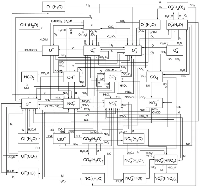
cosmic rays. The model includes molecular and eddy diffu-sion in the vertical direction. For a recent detailed descrip-tion of the model, see Verronen et al. (2005) and references therein. Figure 1 presents a diagram of the negative ion re-action paths considered in the SIC model. Note, however, that photodetachment and photodissociation reactions are not shown in the diagram.
For this study, two new neutrals were added as unknowns: O2(11g) and H2O2. Both of these have strong diurnal
vari-ation in the stratosphere and lower mesosphere. The chem-ical scheme was updated accordingly. O2(11g) is produced
by photodissociation of ozone and is then deactivated in a reaction with molecular oxygen or by quenching (see, e.g. Brasseur and Solomon, 1986). The reaction rate coefficients for the loss reactions were taken from Sander et al. (2003) and Thomas et al. (1983), respectively. Note that the ionic reactions of O2(11g) were already included in the model and
are given by Turunen et al. (1996). For H2O2, we added the
loss by photodissociation using cross sections from Sander et al. (2003). The other reactions important to H2O2were
already included in the model.
2.1 Modelling of the sunset of 23 October 1989
The modelling started with an initialisation of the model, i.e. the same day (mid-October conditions) was modelled over and over again until a repeatable diurnal cycle was reached. This initialisation then provided the starting concentrations for the SPE modelling, which was run from 18 October, 00:00 UT (about 37 h before the initial onset of the SPE) until 23 October, 24:00 UT. Ionization rates due to proton precipi-tation were calculated using proton flux measurements of the GOES-7 satellite as input, in the manner described by Ver-ronen et al. (2005). For the present study, the location of all modelling is that of the EISCAT VHF radar in Tromsø, Nor-way (69.59◦N, 19.23◦E). The model was run for a restricted altitude range of 20–120 km instead of taking the default up-per limit at 150 km, and the results were saved with a 5-min time resolution.
The SPE started in the afternoon (UT) of 19 October 1989. Measured fluxes of high-energy protons peaked dur-ing the next day, with the E>30 MeV proton flux reach-ing values higher than 108m−2s−1sr−1, which means an in-crease by 5 orders of magnitude above the quiet-time values. Subsequent peaks occurred on 23 and 25 October, with the
>30 MeV proton flux values exceeding 107m−2s−1sr−1. At
the D-region altitudes, the calculated ionization rates from the onset of the event until the end of 23 October varied be-tween 108and 1010m−3s−1. Thus, the ionization due to the SPE clearly exceeded the quiet-time ionization sources (see, e.g Hargreaves, 1992, p. 230). In the model, we have ne-glected the ionization by hard X-rays (0.1–0.8 nm), a highly variable source which can significantly contribute to the D-region ionization. However, during a strong SPE it is rea-sonable to assume that the ionization is dominated by the precipitating protons.
P. T. Verronen et al.: Negative charge transition in the D-region during sunset 189
Figures
O/O3 O/O3 H2O,M H2O H2O/H2 H2O,M H2O,M H2O,M H2O,M M M O3 M CO2,M CO2,M O2 2O2 O H H H H H H O O O O O O3 O3 O3 O3 CO2 CO2 CO2 CO2 NO NO NO NO/NO2 NO NO NO/H HCl Cl HCl Cl HCl Cl Cl Cl ClO ClO HCl,M ClO ClO ClO ClO HCl/Cl/ClO HCl / Cl / ClO CO2 O2,N2 O3/2O2 O/H O/NO/O2 (1∆g)/M O2(1∆g) N2 NO2 NO2 NO2 HNO2 NO2 NO2 O/NO OH– CO3– HCO3– CO4 – Cl– ClO– NO3–* NO3– NO2– CO3–(H2O) CO3–(H2O)2 Cl–(H2O) Cl–(CO2) Cl–(HCl) NO3–(H2O) NO3–(H2O)2 O– O– O3– O4 – O2– O2–(H2O) O2–(H2O)2 O3–(H2O) OH–(H2O) e (H2O) H2O,M H2O,M NO2 M H 2O,M M NO2–(H2O) NO3–(HCl) NO3–(HNO3) NO3–(HNO3)2 M HNO3 H2O,M O2 O 3 NO HCl,M HNO3,M HNO3 NO/ NO2 CO2 H2O,M M CO2,M HCl M O2 M NO2 HCl HNO3, M M H2O,M HCl / Cl /ClO H2O CO2 NO2O3 NO2 HNO3 NO2 HNO3 M M CO2 ,O2 O2,M HNO3 CO2 HNO3 M HNO3/ N2O5 MFig. 1. Block diagram for the negative ion scheme of the SIC model. The various ions in the blocks are either the
reactants or the final products of the reactions sketched by the connecting arrows. The arrows are labelled with the
neutral constituents taking part in the reactions. Note, that photodetachment and photodissociation reactions are not
shown in the diagram.
21
Fig. 1. Block diagram for the negative ion scheme of the SIC model. The various ions in the blocks are either the reactants or the final products
of the reactions sketched by the connecting arrows. The arrows are labelled with the neutral constituents taking part in the reactions. Note that photodetachment and photodissociation reactions are not shown.
We are especially interested in the sunset of 23 October because of the EISCAT measurements made between 12:00 and 18:00 UT in a special lower D-region mode. However, it is important to model the whole history of the event be-fore the radar experiment, because changes in the neutral at-mosphere caused by the SPE, which can be cumulative and long-lasting, are likely to be important to the sunset transition characteristics. Odd nitrogen (NOx=N+NO+NO2) is
pro-duced in significant amounts through dissociation of molec-ular nitrogen via particle impact and ion chemistry (Rusch et al., 1981). Also odd hydrogen (HOx=H+HO+HO2) is
pro-duced, through hydrate ion chemistry following the ioniza-tion (Solomon et al., 1981). As already menioniza-tioned, NO plays and important part in determination of the ion balance. In addition, enhancements in NOxand HOxsubsequently lead
to an ozone decrease through catalytic reactions (see, e.g. Brasseur and Solomon, 1986, p. 291–299). While NOx is
expected to affect ozone in the upper stratosphere, an HOx
increase will lead to an ozone depletion at D-region alti-tudes. Ozone changes have an effect, e.g., on the produc-tion of O−3, which is an important intermediate ion for the “terminal” ions CO−3 and NO−3. The twilight transition of negative charge will also be affected, because ozone is in a photochemical balance with atomic oxygen and is the source of O2(11g), both of which are involved in electron
detach-ment reactions. Further, the ozone depletion is expected to be strongest during sunrise and sunset times (Verronen et al., 2005). With our combined ion and neutral chemistry model, we are able to account for the neutral atmospheric changes caused by the SPE.
During the sunset of 23 October, the proton fluxes stayed relatively constant, although at a highly elevated level when contrasted with quiet-time levels. At altitudes above 65 km the calculated ionization rates, based on GOES
190 P. T. Verronen et al.: Negative charge transition in the D-region during sunset 13 13.5 14 14.5 15 15.5 16 16.5 17 85 95 105 SZA [deg] a) Altitude [km] 1.0 0.8 0.6 0.4 0.2 0.0 b) 13 13.5 14 14.5 15 15.5 16 16.5 17 40 50 60 70 80 90 100 Altitude [km] UT hour on Oct 23, 1989 1.0 0.8 c) 13 13.5 14 14.5 15 15.5 16 16.5 17 40 50 60 70 80 90 100
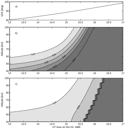
Fig. 2. a) Solar zenith angles for the sunset of October 23. b) Calculated scaling factors for UV-dependent reaction rate
coefficients. c) Same as b) but for VIS-dependent reactions. The same contour lines are shown in both b) and c), but for practical reasons only two of the lines are labelled in the bottom panel.
22
Fig. 2. (a) Solar zenith angles for the sunset of 23 October. (b) Calculated scaling factors for UV-dependent reaction rate coefficients. (c) Same as (b) but for VIS-dependent reactions. The same contour lines are shown in both (b) and (c), but for practical reasons only two of
the lines are labelled in the bottom panel.
measurements, show a steady reduction by 5–15% between 12:00 and 18:00 UT. Therefore, the sunset transition under study was not significantly disturbed by sudden changes in the proton forcing.
In the SIC model, photodetachment is considered for O−, O−2, O−3, OH−, CO−3, NO−2, and NO−3 and photodissocia-tion for O−3, O−4, CO−3, CO−3(H2O), and CO−4. The
pho-todissociation of CO−3 (and CO−3(H2O)) is important for
twi-light transitions because it releases O−, which then, in turn, rapidly releases an electron (Peterson, 1976). In addition to photon-driven reactions, there are a number of two-body re-actions which release an electron, involving O−, O−2, O−3, OH−, and Cl−. These reactions and their rate coefficients are given by Turunen et al. (1996), except the photodissoci-ation of CO−3(H2O) which comes from Peterson (1976). For
the photodetachment and photodissociation reactions the rate coefficients are given in “full-light” conditions; in the model we scale them based on the illumination level, in a manner similar to del Pozo et al. (1999). The scaled coefficient ks is
calculated from the “full-light” coefficient k as
ks = F F0
k, (3)
where F is the wavelength-integrated solar flux at a certain altitude at a certain time. F0is a reference flux pre-calculated
for the same altitude but for solar zenith angle of 45◦. For NO−3 photodetachment the fluxes are integrated from 99 to
318 nm (Reid, 1987), while for photodetachment and pho-todissociation of other ions the integration is done from 99 to 422 nm. Figure 2 shows the calculated UV-dependent (<318 nm) and VIS-dependent (<422 nm) scaling factors (FF
0), as well as the solar zenith angles for the sunset of
23 October. The UV and VIS wavelengths are attenuated differently, especially at high solar zenith angles. UV attenu-ation is strong and during sunset UV fluxes gradually reduce to zero well before the ray interception by the solid Earth oc-curs. In contrast, VIS radiation is only partially attenuated before the interception, when it is practically “switched off”. Solar flux values at each altitude are determined us-ing the well-known Beer-Lambert absorption law, with the daily above-atmosphere fluxes provided by the SOLAR2000 model, version 2.23 (Tobiska et al., 2000). Calculation of op-tical depth is required, and for high zenith angles it is neces-sary to take into account the spherical geometry of the atmo-sphere. In our model, the optical depth calculation follows a procedure described by Rees (1989, p. 12–13). Note that in the calculations we do not take into account refraction, the effect of which is negligible for all ray paths, except maybe those with a tangent point very close to the Earth’s surface (Reid, 1987). The main absorbing gases are molecular oxy-gen and ozone. The MSISE90 model provides O2
concentra-tion profiles down to the ground level (Hedin, 1991), while for O3we use the model results, so that the optical depth
P. T. Verronen et al.: Negative charge transition in the D-region during sunset 191
Altitude [km]
log10( Ozone concentration [m−3] )
a) 14 15 16 17 16.5 15.5 14.5 13.5 12 13 14 15 16 17 18 50 60 70 80 UT hour on Oct 23, 1989 Altitude [km] log10( NO concentration [m−3] ) b) 11.5 11 12 13 14 14.5 14.5 14.5 13.5 12.5 12 13 14 15 16 17 18 30 40 50 60 70
Fig. 3. Modelled variation of a) ozone and b) nitric oxide concentrations during the sunset of October 23, 1989.
18 19 20 21 22 23 24 0 30 60 90 120
Cutoff energy [MeV]
Day of October, 1989 a) 18 19 20 21 22 23 24 0 25 50 75 100 Cum. prod. of NO [%] Day of October, 1989 b)
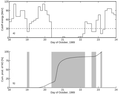
Fig. 4. a) Calculated magnetic rigidity cutoff energies for the rocket measurement location. b) Cumulative production
of NO at 50 km from October 18 to October 23, 05:00 UT (model results, no cutoff applied). The shaded areas indicate the times of NO production when taking into account the variation with time of the cutoff energy.
23
Fig. 3. Modelled variation of (a) ozone and (b) nitric oxide concentrations during the sunset of 23 October 1989.
proton precipitation, as well as the normal diurnal variation which is substantial in the upper stratosphere and above (see Fig. 3a). However, ozone values below the lower altitude limit of the model at 20 km are also needed because for so-lar zenith angles so-larger than 90◦the ray path passes through these lower altitudes. In the model we use values from Shi-mazaki (1984) and Brasseur and Solomon (1986) for these altitudes, assuming a fixed ozone profile throughout the mod-elling. This assumption is reasonable because 1) at altitudes below about 40 km there is no diurnal variation of ozone and 2) even for large SPEs the effects are typically not significant below ∼30 km.
3 Measurements
3.1 Electron density from EISCAT VHF incoherent scatter radar
Incoherent scatter radars can provide altitude profiles of ionospheric quantities, such as electron density. The tech-nique includes transmitting a power pulse, which is then scat-tered in the ionosphere, so that the returned power can be measured. Several experiment modes were used during the SPEs of 1989; these are described in, for example, Collis and Rietveld (1990).
On 23 October the VHF radar was operated in the spe-cial D-region mode “GEN-11” (Turunen, 1986). The an-tenna was tilted 45◦ towards north, so that the lower alti-tude limit within the radar range was further lowered from 70 km to 50 km. However, due to instrumental limitations the true lower limit of measurements was 54 km (Collis and Ri-etveld, 1990). The quiet-time electron densities in the lower
D-region, below 70 km, are of the order of 107–108m−3(see, e.g. Hargreaves, 1992, p. 231). For these kinds of small val-ues the EISCAT signal-to-noise ratio is too low for measure-ments to be practical (Turunen, 1993). However, in this case the SPE-elevated ionization levels allowed for observations reaching stratopause altitudes.
The radar in Tromsø, Norway (69.59◦N, 19.23◦E) was operated from 12:00 UT until 18:00 UT, measuring the sunset conditions in the D-region. The altitude resolution of the measurements was ≈0.75 km for the tilted antenna (≈1.05 km for a vertical) and the basic time resolution was 10 s. Before the analysis, the data were post-integrated over 5 minutes and interpolated to 1-km grid. The error of the post-integrated data depends on the received power, i.e. for lower electron densities the uncertainty is larger, but is typi-cally better than 10% (Collis and Rietveld, 1990).
3.2 Cosmic radio noise absorption from Kilpisj¨arvi riome-ter
Riometers measure ionospheric absorption of cosmic radio noise, typically at frequencies of 20–60 MHz. Cosmic radio noise is of galactic origin and is considered to be constant over long periods of time, so that any changes in the signal observed on the ground are due to changes in ionospheric absorption. The absorption depends upon electron-neutral collision frequency, which, in turn, depends upon electron density and temperature. Typically, most of the absorption occurs in D-region altitudes, i.e. below 90 km. Riometers are relatively cheap, easy to operate, and can continuously measure the integrated ionization levels of the overhead iono-sphere. Interpretation of measurements includes determina-tion of a quiet-day curve (QDC), which is then subtracted
192 P. T. Verronen et al.: Negative charge transition in the D-region during sunset Altitude [km] log 10( Ozone concentration [m −3] ) a) 14 15 16 17 16.5 15.5 14.5 13.5 12 13 14 15 16 17 18 50 60 70 80 UT hour on Oct 23, 1989 Altitude [km] log 10( NO concentration [m −3] ) b) 11.5 11 12 13 14 14.5 14.5 14.5 13.5 12.5 12 13 14 15 16 17 18 30 40 50 60 70
Fig. 3. Modelled variation of a) ozone and b) nitric oxide concentrations during the sunset of October 23, 1989.
18 19 20 21 22 23 24 0 30 60 90 120
Cutoff energy [MeV]
Day of October, 1989 a) 18 19 20 21 22 23 24 0 25 50 75 100 Cum. prod. of NO [%] Day of October, 1989 b)
Fig. 4. a) Calculated magnetic rigidity cutoff energies for the rocket measurement location. b) Cumulative production
of NO at 50 km from October 18 to October 23, 05:00 UT (model results, no cutoff applied). The shaded areas indicate the times of NO production when taking into account the variation with time of the cutoff energy.
23
Fig. 4. (a) Calculated magnetic rigidity cutoff energies for the rocket measurement location. (b) Cumulative production of NO at 50 km from
18 October to 23 October 05:00 UT (model results, no cutoff applied). The shaded areas indicate the times of NO production when taking into account the variation with time of the cutoff energy.
from measurements, so that the final absorption data by ri-ometers are relative in nature. For a description of riometer techniques and measurements, see, e.g. Ranta et al. (1983). In this study we have used measurements of the Kilpisj¨arvi riometer (69.05◦N, 20.78◦E, f =30 MHz), located in north-ern Finland, about 85 km east of the location of the EISCAT radar.
3.3 Nitric oxide from a Southern Hemispheric rocket flight
There is not much information available on polar nitric oxide during the October 1989 SPE. The only measurements we are aware of are those by Zadorozhny et al. (1994), who flew a M-100B meteorological rocket on 23 October, at 05:00 UT, in the Southern Hemisphere at 55.62◦S, 50.18◦E. The time of the measurement is well suited for comparison with our modelling, because it is more than two days after the peak forcing by protons and only 7 h before the beginning of the EISCAT electron density measurements. On the other hand, the illumination conditions are quite different from those of our modelling location in the Northern Hemisphere. The so-lar zenith angle for the time and location of the rocket flight is about 55◦while at the modelling location the smallest zenith
angle is about 81◦ at 10:25 UT. Although NOx has a
rel-atively long photochemical lifetime, there is a strong diur-nal variation between NO and NO2in the lower mesosphere
and stratosphere. During daytime a photochemical equilib-rium exists but at night most of NO is converted to NO2
through a reaction with O3 (see Fig. 3b). For this reason,
we choose the modelled 10:25 UT NO profile to be com-pared with the rocket measurement. In addition to different illumination conditions, meteorological conditions are
differ-ent in the Southern Hemisphere than in the Northern. In the south, the polar vortex is breaking up, while in the north it is forming. This might lead to important differences in NO be-cause of the possible accumulation of NO inside the southern vortex during the preceding winter months, due to absence of photodissociation and vertical transport (see, e.g. Siskind et al., 1997). Nevertheless, we pursue the comparison be-cause the high production of NOx, due to the SPE, is likely
to have a significant impact on the NO levels at the D-region altitudes. An indication of this is given by another, pre-SPE rocket measurent by Zadorozhny et al. (1994) on 12 Octo-ber (57.08◦S, 45.04◦E), which clearly shows lower values of NO than the observation during the SPE on 23 October, especially in the lower mesosphere and upper stratosphere. In Sect. 4.1 we will show that the observed and modelled, during-SPE altitude profiles have a very similar shape, which is another indication of the dominant role of SPE-produced NO.
In the stratosphere and lower mesosphere the photochem-ical lifetime of NOx, which is determined by
photodissocia-tion of NO, is relatively long compared to the duraphotodissocia-tion of the SPE (Zadorozhny et al., 1994). Therefore, most of the NOx
produced during the SPE is still present on 23 October. In the upper mesosphere and lower thermosphere, the lifetime of NOxis of the order of 1 day in solar illuminated conditions
(Barth et al., 2001), so that a part of the SPE-produced NOx
will have been destroyed before the rocket measurement was made. In summary, the measured and modelled NO profiles should be most comparable in the lower mesosphere, while at higher altitudes the different illumination conditions between the two locations may have significantly different influences on the NOxproduced during the SPE.
P. T. Verronen et al.: Negative charge transition in the D-region during sunset 193 1013 1014 1015 1016 30 40 50 60 70 80 90 100 NO concentration [m−3] Altitude [km]
Fig. 5. NO concentration profiles. Modelling results for October 18 (dashed line) and 23 (solid line) at 10:25 UT are
shown as well as rocket data (stars) from Zadorozhny et al. (1994) including the 85% error margins. The dash-dot line shows the model result for October 23 when applying a higher production of NO by secondary electrons.
UT hour on Oct 23, 1989 Altitude [km] 3 2 1 0 −1 −2 −3 −4 12 13 14 15 16 17 18 45 50 55 60 65 70 75 80 85
Fig. 6. Modelled negative ion to electron ratio, log10(
n−
i
n−
e), during the sunset of October 23. The sharp changes seen
around 16:00 UT indicate the times of Earth’s shadow covering corresponding altitudes.
24
Fig. 5. NO concentration profiles. Modelling results for 18 October (dashed line) and 23 (solid line) at 10:25 UT are shown, as well as rocket
data (stars) from Zadorozhny et al. (1994), including the 85% error margins. The dash-dot line shows the model result for 23 October when applying a higher production of NO by secondary electrons.
Modelling results by Jackman et al. (1995) indicate that the absolute increase of NOy (=N+NO+NO2 in the
meso-sphere) during the October 1989 SPE was essentially the same in both hemispheres. However, because our modelling location and the location of the rocket flight have markedly different magnetic latitudes, they should experience different proton forcing due to differences in magnetic rigidity cutoff, which determines the minimum energy required for a proton to reach a certain geographic location (see, e.g. Hargreaves, 1992, p. 355). To check if this was the case, we calculated the rigidity cutoff energies at the two locations for the du-ration of the SPE using a method which depends upon the measured Kpmagnetic index (see Rodger et al., 2006, for a
description of the method). Our modelling location is well within the magnetic polar cap so that there is effectively no cutoff at any time. At the location of the rocket flight, which is near the edge of the magnetic polar cap, the cutoff ener-gies, shown in the upper panel of Fig. 4, are high for most of the event and display large variations. However, it turns out that the high cutoffs have a relatively small effect on the total NO production in this case (see Sect. 4.1 for a discussion).
4 Results and discussion 4.1 Nitric oxide
Figure 5 compares the modelled and rocket-measured NO profiles, which are very similar in shape. The maximum of NO is at 45–60 km, a minimum is at 70–80 km, and above 80 km the concentration again increases. The modelled con-centrations are within the error margins of the
measure-ments at all altitudes and the agreement between the mea-sured and modelled NO values is very good at the altitudes studied by riometers and EISCAT radar, i.e. between 60 and 80 km. However, the difference in concentration is quite sub-stantial around 50 km, where the measured amount of NO (≈2×10¹⁵m−3) is four times higher than the modelled value (≈5×10¹⁴m−3). We discuss the possible reasons for this
difference below.
The main part of the energy input and NO production by protons occurs between 40 and 80 km, where the modelling result for NO is independent of its initial amount (assum-ing that the initial values before the SPE are lower than those measured after the onset of the SPE). Therefore, if we assume that there is no additional production of NO, the reason for the lower model values might be in the assumptions behind the SIC-modelled production of NO by protons. It should be noted that above 80 km, where the proton forcing has a smaller effect, a better agreement with the measurements was obtained by using a downward NO flux of 4×10¹³m−2s−1 at the upper boundary of the model (120 km) during both ini-tialisation and modelling.
Assuming that the majority of the NO produced by the SPE was not destroyed before 23 October, Zadorozhny et al. (1994) estimated the concentration of NO at 50-km altitude from
[NO] = C
Z
Pidt, (4)
where Pi is the calculated ionization rate and C is a
con-stant varying between 1.2 and 1.6 (see, e.g. Porter et al., 1976; Rusch et al., 1981). Integrating from the beginning of the SPE until the rocket flight time, they calculated [NO] to
194 P. T. Verronen et al.: Negative charge transition in the D-region during sunset 1013 1014 1015 1016 30 40 50 60 70 80 90 100 NO concentration [m−3] Altitude [km]
Fig. 5. NO concentration profiles. Modelling results for October 18 (dashed line) and 23 (solid line) at 10:25 UT are
shown as well as rocket data (stars) from Zadorozhny et al. (1994) including the 85% error margins. The dash-dot line shows the model result for October 23 when applying a higher production of NO by secondary electrons.
UT hour on Oct 23, 1989 Altitude [km] 3 2 1 0 −1 −2 −3 −4 12 13 14 15 16 17 18 45 50 55 60 65 70 75 80 85
Fig. 6. Modelled negative ion to electron ratio, log10(n
−
i
n−
e), during the sunset of October 23. The sharp changes seen
around 16:00 UT indicate the times of Earth’s shadow covering corresponding altitudes.
24
Fig. 6. Modelled negative ion to electron ratio, log10(n
− i
n−e
), during the sunset of 23 October. The sharp changes seen around 16:00 UT indicate the times of the Earth’s shadow covering corresponding altitudes.
be 1.1−1.4×10¹⁵m−3without taking into account the effect of magnetic cutoff. Using the same approach for our mod-elling results, we calculated [NO] to be 6.7−9.3×10¹⁴m−3, which is about 35% lower, partly due to different neutral at-mospheres and ionization rate calculation routines used. The proton energy required for reaching 50-km altitude is about 30 MeV. Integrating the NO production only at times when the cutoff energy (shown in the upper panel of Fig. 4) is smaller than 30 MeV results in about a 20% reduction in the final concentration at 05:00 UT. The applied cutoff has a moderate effect because, as shown in the bottom panel of Fig. 4, most of the NO production occurs on 20 October, when the proton flux was highest and the cutoff was at its lowest. Therefore, in the lower mesosphere the total NO pro-duction by the SPE on the modelling location should be com-parable to that at the rocket flight location.
The SIC equivalent of C (in Eq. 4) can be estimated from the model results by considering the different pathways lead-ing from ionization to NOxproduction through dissociation
of N2by protons and secondary electrons, as well as a
num-ber ion chemical reactions. By dividing the NOxproduction
rate by the ionization rate, the constant C is found to be about 1.15 at 50 km, i.e. in the lower limit of its theoretical range. An adjustable parameter in the model is the production of atomic nitrogen by secondary electrons, which is set to 0.8 times the ionization rate, equal to the lower limit given by Rusch et al. (1981). Figure 5 shows that by using the up-per limit of this parameter, 1.21 (i.e. C≈1.56), the resulting amount of NO at 50 km is about 7×10¹⁴m−3, which is still almost three times lower than the measured value.
Ionization leads to atomic nitrogen production first, and here the branching between N(2D) and N(4S) states is
im-portant because the former produces NO while the latter de-stroys it (Brasseur and Solomon, 1986, p. 267). Zipf et al. (1980) have reported this branching to be close to 0.54, favouring N(2D), but there is some uncertainty and this ra-tio is commonly used as a fitting parameter in models. In our model we use a value of 0.6. As a sensitivity test, we increased the ratio to 0.75 and repeated the whole SPE mod-elling. The results (not shown) indicate that at 50 km the amount of NO is quite insensitive to the change while at 65– 80 km the NO values clearly exceeded the measured ones.
Zadorozhny et al. (1994) mention production by relativis-tic electron precipitation as a possible reason for the high amounts of NO measured at 50 km. Since the uncertainties in the modelled SPE-driven production of NO are not able to fully explain the difference between modelling and the rocket measurements, an additional production source seems quite probable, especially if taking into account that the NOx
(=NO+NO2) production of the SIC model has been validated
during another SPE by the GOMOS instrument aboard the Envisat satellite (Verronen et al., 2005).
4.2 Negative ion concentrations
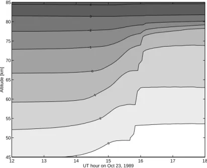
In D-region research, it is usual to show the negative ion to electron ratio, λ. A graph of this parameter, based on the model results, is presented as a function of time and altitude in Fig. 6 for the sunset hours of 23 October. It clearly demon-strates the transition of negative charge from ions to electrons during the sunset. Before the sunset, the transition altitude, where negative ion and electron concentrations are equal, is at ≈67 km, while after the sunset it is at ≈78 km.
P. T. Verronen et al.: Negative charge transition in the D-region during sunset 195 107 108 109 1010 1011 45 50 55 60 65 70 75 80 85 Number density [m−3] Altitude [km] 14:00 UT 107 108 109 1010 1011 45 50 55 60 65 70 75 80 85 Number density [m−3] Altitude [km] 15:30 UT 107 108 109 1010 1011 45 50 55 60 65 70 75 80 85 Number density [m−3] Altitude [km] 17:00 UT
Fig. 7. Modelled density profiles of the main negative ions before, during, and after the sunset of 23 October. Dashed line, solid line, and
dash-dot line indicate O−2, CO−3, and NO−3, respectively.
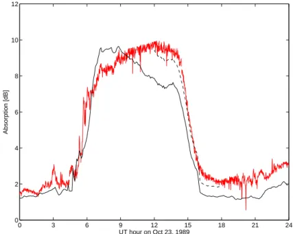
0 3 6 9 12 15 18 21 24 0 2 4 6 8 10 12 UT hour on Oct 23, 1989 Absorption [dB]
Fig. 8. Cosmic radio noise absorption as calculated from the model results (solid black line) and as measured by the Kilpisj¨arvi 30-MHz
riometer (solid red line) 85 km east of the modelling location. Also shown is the calculated absorption when taking into account the estimated constant relativistic electron precipitation (dashed black line).
Figure 7 shows the model density profiles of the main neg-ative ions before, during, and after the sunset transition. The main daytime ions in the lower mesosphere are NO−3 and CO−3. Around 65 km these two are more or less equal with
O−2 which is the main ion at higher altitudes. There is also a multitude of other ions (including cluster ions) present, es-pecially at lower altitudes, but with smaller concentrations. During the sunset a clear change in the ion composition
196 P. T. Verronen et al.: Negative charge transition in the D-region during sunset 0 1 2 3 4 x 10¹⁰ 50 60 70 80 90 100 Altitude [km] 14:00 UT 0 1 2 3 4 x 10¹⁰ 50 60 70 80 90 100 15:00 UT 0 1 2 3 4 x 10¹⁰ 50 60 70 80 90 100 Altitude [km] 15:20 UT 0 1 2 3 4 x 10¹⁰ 50 60 70 80 90 100 15:50 UT 0 1 2 3 4 x 10¹⁰ 50 60 70 80 90 100 Density [m−3] Altitude [km] 16:00 UT 0 1 2 3 4 x 10¹⁰ 50 60 70 80 90 100 Density [m−3] 16:15 UT
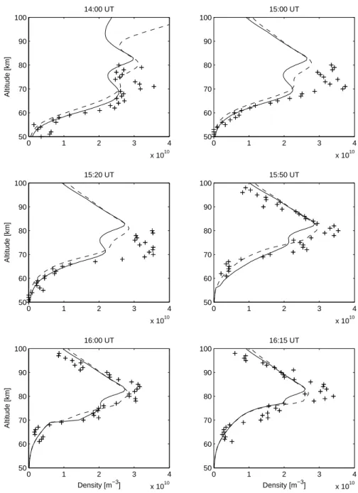
Fig. 9. Raw electron density profiles for selected times before, during, and after the sunset of October 23. EISCAT
measurements (+) as well as modelling results with model-determined NO (solid line) and with manually increased NO
(dashed line) are shown.
26
Fig. 9. Raw electron density profiles for selected times before, during, and after the sunset of 23 October. EISCAT measurements (+), as
well as modelling results with model-determined NO (solid line) and with manually increased NO (dashed line), are shown.
occurs, which is related to the negative charge transition. NO−3 increases at all altitudes due to a reduction in its pho-todetachment. Also photodissociation of CO−3 decreases, at a later time, and its concentration increases at altitudes above 60 km. O−2 decreases at altitudes below 70 km, while NO−3 and CO−3, for which the main loss processes are the detach-ment/dissociation reactions, hold a larger and larger portion of the negative charge as the sunset advances. After sunset, when a nighttime balance is reached, NO−3 is clearly the main ion.
4.3 Cosmic radio noise absorption
Each run of the SIC model is based on a neutral background atmosphere given by the MSISE90 model and provides con-centration profiles of neutral and ionic species. Cosmic radio noise absorption can be estimated from the modelling results by following Banks and Kockarts (1973, Part A, p. 194) and calculating the electron collision frequencies of N2, O2, and
He from MSIS and of O and H from SIC, using the neu-tral temperature profile of MSIS, which we can assume to be equal to the electron temperature below 100 km. Elec-tron density is obtained from SIC by subtracting the sum of negative ion concentrations from the sum of positive ion
P. T. Verronen et al.: Negative charge transition in the D-region during sunset 197
concentrations. Finally, we use the method of Sen and Wyller (1960) to compute differential absorption dL/dh and inte-grate with respect to height. This method takes the opera-tional frequency of the riometer and assumes a dipole ap-proximation for the geomagnetic field to obtain an electron gyrofrequency at the respective altitude and latitude.
Figure 8 shows the calculated absorption for 23 October compared to that measured by the Kilpisj¨arvi 30-MHz ri-ometer (located 85 km East of the modelling location), both of which show two distinct levels, 1–3 dB at night and 7– 10 dB during day. The daytime behaviours, from 07:00 to 14:00 UT (10:25 UT corresponds to local time noon), be-tween the modelled and observed absorptions, differ signifi-cantly. The riometer shows a gradual increase between sun-rise until the beginning of sunset, while calculated values follow the proton forcing, peaking at 07:00–09:00 UT and then gradually decrease until reaching a lower level at about 13:00 UT. The calculated absorption values are clearly lower than those measured at daytime (after 10:00 UT), as well as during and after the sunset. However, the sunset behaviour is well modelled, in time scale as well as in steepness of the transition.
At nighttime, when the D-region electron density is low, the contribution of upper altitudes can be important to total absorption, especially if auroral precipitation occurs. From EISCAT measurements (CP2 mode, from 18:00 UT onwards, not shown) it is evident that there was auroral electron pre-cipitation after sunset, resulting in significantly higher elec-tron density values at altitudes above 90 km compared to our modelling. By replacing the modelled densities with the measured ones and then repeating the absorption calcula-tion from 18:00 to 24:00 UT, the resulting absorpcalcula-tions were clearly closer to those measured by the riometer. Therefore, a part of the after-sunset difference between the measured and modelled absorption can be explained by auroral elec-tron precipitation. At daytime, the majority of the absorption comes from the D-region altitudes, such that typical auroral electron precipitation, if present, could explain only a small portion of the difference. However, in the following sections we will show that high-energy electron precipitation is a pos-sible cause for the daytime differences.
4.4 Electron densities
For comparison, the modelled electron densities were con-verted to raw electron densities Neraw. The backscattered power of EISCAT radar is a direct measure of Neraw, which, on the other hand, is a function of the electron density and the total concentration of negative ions (see, e.g. del Pozo et al., 1999, and references therein for more details on the conversion).
Electron density profiles for selected times during the sun-set are shown in Fig. 9. The shapes of the measured profiles vary significantly during sunset at altitudes below 80 km. These variations are well represented by the model. For the profiles of 14:00 UT and from 15:50 UT on, the magnitudes agree within the EISCAT 10% statistical uncertainty
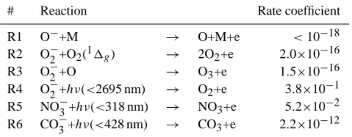
mar-Table 1. Most important electron-detachment reactions from the
SIC model. Sources of the rate coefficients are listed in Turunen
et al. (1996). Units are m3s−1for R1–R3 and s−1for the other
reactions.
# Reaction Rate coefficient
R1 O−+M → O+M+e <10−18 R2 O−2+O2(11g) → 2O2+e 2.0×10⁻¹⁶ R3 O−2+O → O3+e 1.5×10⁻¹⁶ R4 O−2+hν(<2695 nm) → O2+e 3.8×10⁻¹ R5 NO−3+hν(<318 nm) → NO3+e 5.2×10⁻² R6 CO−3+hν(<428 nm) → CO3+e 2.2×10⁻¹²
gins at most altitudes. Most significant differences, which are clearly larger than the 10% margin, are in the 15:00 UT and 15:20 UT profiles at altitudes above 65 km. Since the negative charge transition during the sunset should result in decreasing rather than increasing electron density, a possi-ble reason for the observed higher densities is an additional ionization source.
Considering the temporal behaviour, Fig. 10 shows the sunset electron densities for altitudes of 65, 72, and 80 km. At 80 km there is no clear transition in either the measure-ments or in the modelling. This is expected because the electrons are dominant over negative ions at this altitude. The modelled density decreases after sunset, partly due to the gradual decrease in proton forcing, while the measured density stays more or less at the same level. At lower alti-tudes there are clear transitions, which begin at about 15:30 and 14:30 UT, at 72 and 65 km, respectively. At 65 km, the change is gradual until 16:00 UT, when there is a “drop off”, i.e. a sudden decrease of electron density between 15:55 and 16:00 UT, corresponding to the Earth’s shadow covering this altitude. This drop off is also seen in the data, although not as pronounced. The initial gradual change and drop-off end constitute a two-step process, similar to what has been ob-served in sunrise conditions (Collis and Rietveld, 1990). This indicates that the transition is dependent on both the UV and VIS solar radiation. At 72 km, the transition is steeper than at 65 km. The drop off occurs 5 min later than at 65 km and is not visible in the data, although such a step could be hidden by the 10% uncertainty. The measured values show a con-tinuing transition until 16:30 UT, a feature that is within the uncertainty limits and is not confirmed by the model. De-spite the differences in the magnitudes of electron density, the comparison shows that the model is able to represent the sunset transition reasonably well.
The model results indicate that the sunset transition of negative charge is a combination of VIS and UV sources. The main processes of negative ions releasing an electron are listed in Table 1 and the detachment rates of these reac-tions at 65 and 72 km are plotted in Figs. 11a–b. All these reactions are photon-driven either directly (R4–R6) or indi-rectly. R2 and R3 are controlled by UV-related changes in
198 P. T. Verronen et al.: Negative charge transition in the D-region during sunset 12 13 14 15 16 17 18 0 2 4 6x 10
10 Raw electron density at 80 km
Density [m −3 ] 12 13 14 15 16 17 18 0 1 2 3 4x 10
10 Raw electron density at 72 km
Density [m − 3 ] 12 13 14 15 16 17 18 0 1 2 3 4x 10
10 Raw electron density at 65 km
Density [m
−
3 ]
UT hour on Oct 23, 1989
Fig. 10. Sunset behaviour of raw electron densities at selected altitudes from EISCAT measurements (+) and modelling (solid line). In the
middle panel, the model values multiplied by 1.5 are shown (dashed line) to aid the comparison with the measured values.
atomic oxygen and O2(11g), and the fast reaction R1 is also
photon-driven because O− acts as an intermediate species
between photodissociation of CO−3 and fast electron detach-ment (from O−). At 65 km the UV dependence is strong, with reactions R2–R4 contributing. It is worthwhile to note that the effect of the O2(11g) change is larger than that
of atomic oxygen change, and that the effect of NO−3 pho-todetachment is relatively small. Reactions R1, R4, and R6 contribute to the VIS dependence (displaying the drop off at 16:00 UT), with R1 being the most important of these. As noted earlier, the VIS dependence of R1 originates from CO−3 photodissociation. At 75 km, the main VIS dependence comes from R1 and R4, i.e. CO−3 and O−2. The UV depen-dence, which is relatively not as strong as at 65 km, is, for the most part, due to changes in atomic oxygen and O2(11g).
In the case of sunrise, the amount of NO determines the relative size of UV and VIS effects by controlling the bal-ance between NO−3 and CO−3 (Reid, 1987). For our sun-set case, we tested the sensitivity of our model by repeating the sunset calculation with a higher amount of NO. Starting at 11:00 UT, we manually increased the starting concentra-tion by 5 times at all altitudes and then ran the model until 18:00 UT. The results (see Figs. 11c–d) show that, due to NO−3 holding a larger portion of the negative charge, 1) the UV effect is increased relative to the VIS effect at lower al-titudes (where NO−3 and CO−3 are the main daytime ions), 2)
VIS-driven reaction rates R1, R4, and R6 show a more grad-ual decrease before the total “switch off”, especially at higher altitudes, and 3) the photodetachment of NO−3 becomes rela-tively more important. The comparison with measured elec-tron density profiles, shown in Fig. 9, improves, especially at altitudes 75–82 km. At altitudes below 70 or 75 km, de-pending on the UT time, the comparison generally becomes worse or at least does not improve. Except for the 14:00 UT case, where photoionization still operates on NO at higher altitudes, there is no significant effect on electron densities above 82 km. Therefore, we could speculate that the original modelling underestimates the amount of NO between 70 and 85 km. Although the increased concentrations of NO, e.g. [NO] ≈1015m−3at 80 km, exceed the measured values, this could perhaps be explained by the differences in illumination level, which, for the modelling location, is relatively low and favours the downward transport of NO produced at higher altitudes.
4.5 High-energy electron flux
The shape of the measured cosmic radio noise absorp-tion, which does not follow the decreasing proton forc-ing but shows a gradual increase durforc-ing the daylight hours (Fig. 8), could be explained by an additional ionization source. The same kind of behaviour is seen in mea-surements of some other riometer stations (not shown) in
P. T. Verronen et al.: Negative charge transition in the D-region during sunset 199 13 14 15 16 17 0 0.5 1 1.5 2 2.5 3x 10 9 UT hour on Oct 23, 1989 Detach. rate [m −3 s −1 ] c) 13 14 15 16 17 0 1 2 3 4 5x 10 8 UT hour on Oct 23, 1989 d) 13 14 15 16 17 0 1 2 3 4 5x 10 8 b) 13 14 15 16 17 0 0.5 1 1.5 2 2.5 3x 10 9 Detach. rate [m −3 s −1 ] a) R1 R2 R3 R4 R5 R6
Fig. 11. Modelled rates of electron detachment from negative ions at a) 65 km and b) 72 km. The legend, which is the
same for all panels, identifies the reactions listed in Table 1. Panels c) and d) are as a) and b), respectively, but with
manually increased NO.
28
Fig. 11. Modelled rates of electron detachment from negative ions at (a) 65 km and (b) 72 km. The legend, which is the same for all panels,
identifies the reactions listed in Table 1. Panels (c) and (d) are as (a) and (b), respectively, but with manually increased NO.
1013 1014 1015 1016 1017 45 50 55 60 65 70 75 80 85 Number density [m−3] Altitude [km] (a) 1013 1014 1015 1016 1017 45 50 55 60 65 70 75 80 85 Number density [m−3] Altitude [km] (b) 14:00 UT 15:30 UT 17:00 UT
200 P. T. Verronen et al.: Negative charge transition in the D-region during sunset
the northern Fennoscandia area, especially that of Oulu (65.05◦N, 25.54◦E), which shows a daytime increase by ≈25% from a.m. to p.m. hours. The additional source could be auroral electrons, but the discrepancy at 70–80 km be-tween the measured and modelled electron densities (Fig. 9) requires electrons reaching relativistic energies.
By trial and error, we estimated the flux of monoenergetic beam of electrons required to increase the modelled elec-tron densities to the measured level. Choosing the energy and flux, the resulting ionization rate was calculated follow-ing Rees (1989, p. 35–45) and usfollow-ing electron energy-range values from Goldberg et al. (1984) and Berger and Seltzer (1972). The calculated rate was then input in the model, together with the proton forcing, and the sunset modelling was rerun. We found that a combination of 650-keV energy and 1.45×10⁹m−2s−1flux resulted in electron density
lev-els quite close to the EISCAT measurements. This estimated flux is comparable to relatively high fluxes which have been measured during specific electron precipitation events by, e.g., the PET/SAMPEX instrument (Callis et al., 1996). Ob-viously, a monoenergetic and constant-flux beam is hardly a good representative of the real situation, but due to the lack of measurements we are limited to this approach, to provide a rough estimate.
By using the increased electron density profiles, the cal-culated radio noise absorption values, shown in Fig. 8, sig-nificantly increase, and show very good agreement with the riometer measurements. Therefore, it seems that an addi-tional ionization source, most likely high-energy electrons, was present during the afternoon and sunset hours of 23 Oc-tober.
4.6 Spectral width of EISCAT measurements
Del Pozo et al. (1999) studied the rapid change in incoherent scatter radar spectral width during the sunset of 23 October, roughly estimated the sunset change in the oxygen species, and concluded that change in atomic oxygen and to a lesser extent that of O2(11g) could explain the observations. Our
modelling results, shown in Fig. 12, agree with this conclu-sion, for the most part. Atomic oxygen and O2(11g) show
an order of magnitude (or greater) decrease at altitudes below 65 km, from 14:00 UT to 15:30 UT, which is equal to the re-quired reduction estimated by del Pozo et al. (1999). The spectral width is about twice as sensitive to the concentration to atomic oxygen than that of O2(11g) at lower mesospheric
altitudes (see Fig. 8 in del Pozo et al., 1999). Thus, above 65 km, where the absolute reduction of O is equal to or higher than that of O2(11g), the observed spectral width change is
mostly due to the change in O. At lower altitudes, where the absolute change in O2(11g) is clearly larger than that of
atomic oxygen, the contributions of the two constituents may be more comparable.
5 Conclusions
A 1-D neutral and ion chemistry model has been used to in-terpret measurements of nitric oxide, cosmic radio noise ab-sorption, and electron density made during the great proton storm of October 1989, in high ionization conditions. The model and the measurements are generally found to be in good agreement. Although there are still great uncertainties involved, e.g., in the photodetachment rates of ions, with the current knowledge we are able to model the D-region iono-sphere with some success.
For the case considered, the sunset transition of negative charge displays dependency on both visible and ultraviolet solar radiation. The model results show that the UV response comes, for the most part, from atomic oxygen and O2(11g)
changes, with a smaller contribution from NO−3 photodetach-ment, while the VIS dependence is driven by reactions of O−2 and CO−3. The relative magnitude of UV and VIS effects vary with altitude, with UV playing a larger role at lower alti-tudes. These transition characteristics are confirmed by both electron density and cosmic radio noise absorption measure-ments.
These sunset transition characteristics are not sensitive to the momentary ionization level, which determines the abso-lute amount of negative (and positive) charge but does not directly affect the balance between the ions. However, our modelling results are sensitive to the amount of NO which, because of its relatively long photochemical lifetime, de-pends upon the ionization history rather than the momen-tary ionization. It is therefore important for studies like the present one, to either model NO accurately or use measured values. However, this requirement can be quite difficult to fulfill because of the high variability of NO in the auroral regions, where the source is unpredictable and the illumina-tion condiillumina-tions vary significantly with season, and also due to spatial and temporal limitations of available data.
Both the cosmic radio noise and electron density measure-ments indicate a possible presence of an additional ionization source, the effect of which is comparable to the ionization caused by the SPE at altitudes 70–80 km. By estimating a reasonable flux of high-energy electrons and including it in our model, the absolute magnitude of modelled values was found to be in excellent agreement with those measured by both instruments. It seems therefore likely that electron pre-cipitation which reached relativistic energies occurred during the afternoon and sunset hours on 23 October.
According to our modelling results, sunset decreases in the amount of atomic oxygen and O2(11g) are such that they
can be used to explain the observed spectral width changes of incoherent scatter radar measurements, as suggested by del Pozo et al. (1999).
Acknowledgements. The work of P. T. Verronen was partially sup-ported by the Academy of Finland through the ANTARES space
research programme. EISCAT is an International Association
supported by Finland (SA), France (CNRS), Germany (MPG), Japan (NIPR), Norway (NFR), Sweden (VR) and the United King-dom (PPARC). GOES proton flux data were provided by the SPIDR
P. T. Verronen et al.: Negative charge transition in the D-region during sunset 201
online data repository. The authors thank N. Riipi and K. Sorri for updating Fig. 1. P. T. Verronen thanks J. Tamminen for usefull dis-cussions.
Topical Editor M. Pinnock thanks A. M. Zadorozhny and an-other referee for their help in evaluating this paper.
References
Banks, P. M. and Kockarts, G.: Aeronomy, Academic Press, 1973. Barth, C. A., Baker, D. N., and Mankoff, K. D., The northern
au-roral region as observed in nitric oxide, Geophys. Res. Lett., 28, 1463–1466, 2001.
Berger, M. J. and Seltzer, S. M.: Bremsstrahlung in the atmosphere, J. Atmos. Terr. Phys., 34, 85–108, 1972.
Brasseur, G. and Solomon, S.: Aeronomy of the Middle Atmo-sphere, D. Reidel Publishing Company, Dordrecht, 2nd edn., 1986.
Burns, C. J., Turunen, E., Matveinen, H., Ranta, H., and Harg-reaves, J. K.: Chemical Modeling of the Quiet Summer D- and E-regions Using EISCAT Electron Density Profiles, J. Atmos. Terr. Phys., 53, 115–134, 1991.
Callis, L. B., Boughner, R. E., Baker, D. N., Mewaldt, R. A., Blake, J. B., Selesnick, R. S., Cummings, J. R., Natarajan, M., Mason, G. M., and Mazur, J. E.: Precipitation electrons: Evidence for effects on mesospheric odd nitrogen, Geophys. Res. Lett., 23, 1901–1904, 1996.
Clilverd, M. A., Rodger, C. J., Ulich, T., Sepp¨al¨a, A., Turunen, E., Botman, A., and Thomson, N. R.: Modelling a large solar proton event in the southern polar cap, J. Geophys. Res., 110, A09 307, 2005.
Collis, P. N. and Rietveld, M. T.: Mesospheric observations with the EISCAT UHF radar during polar cap absorption events: 1. Electron densities and negative ions, Ann. Geophys., 8, 809–824, 1990.
del Pozo, C. F., Turunen, E., and Ulich, T.: Negative ions in the au-roral mesosphere during a PCA event around sunset, Ann. Geo-phys., 17, 782–793, 1999,
SRef-ID: 1432-0576/ag/1999-17-782.
Goldberg, R. A., Jackman, C. H., Barcus, J. R., and Soraas, F.: Nighttime auroral energy deposition in the middle atmosphere, J. Geophys. Res., 89, 5581–5596, 1984.
Hargreaves, J. K.: The solar-terrestrial environment, Cambridge Atmospheric and Space Science Series, Cambridge University Press, Cambridge, UK, 1992.
Hedin, A. E.: Extension of the MSIS Thermospheric Model into the Middle and Lower Atmosphere, J. Geophys. Res., 96, 1159– 1172, 1991.
Jackman, C. H., Cerniglia, M. C., Nielsen, J. E., Allen, D. J., Za-wodny, J. M., McPeters, R. D., Douglass, A. R., Rosenfield, J. E., and Hood, R. B.: Two-dimensional and three-dimensional model simulations, measurements, and interpretation of the Oc-tober 1989 solar proton events on the middle atmosphere, J. Geo-phys. Res., 100, 11 641–11 660, 1995.
Peterson, J. R.: Sunlight photodestruction of CO−3, its hydrate, and
O−3 – The importance of photodissociation to the D region
elec-tron densities at sunrise, J. Geophys. Res., 81, 1433–1435, 1976. Porter, H. S., Jackman, C. H., and Green, A. E. S.: Efficiencies for production of atomic nitrogen and oxygen by relativistic proton impact in air, J. Chem. Phys., 65, 154–167, 1976.
Ranta, H., Ranta, A., Rosenberg, T. J., and Detrick, D. L.: Autumn and winter anomalies in ionospheric absorption as measured by
riometers, J. Atmos. Terr. Phys., 45, 193–202, 1983.
Rees, M. H.: Physics and chemistry of the upper atmosphere, Cam-bridge atmospheric and space science series, CamCam-bridge Univer-sity Press, Cambridge, UK, 1989.
Reid, G. C.: Radar observations of negative-ion photodetachment at sunrise in the auroral-zone mesosphere, Planet. Space Sci., 35, 27–37, 1987.
Reid, G. C., Solomon, S., and Garcia, R. R.: Response of the mid-dle atmosphere to the solar proton events of August–December, 1989, Geophys. Res. Lett., 18, 1019–1022, 1991.
Rietveld, M. T. and Collis, P. N.: Mesospheric observations with the EISCAT UHF radar during polar cap absorption events: 2. Spectral measurements, Ann. Geophys., 11, 797–808, 1993. Rietveld, M. T., Turunen, E., Matveinen, H., Goncharov, N. P., and
Pollari, P.: Artificial periodic irregularities in the auroral iono-sphere, Ann. Geophys., 14, 1437–1453, 1996,
SRef-ID: 1432-0576/ag/1996-14-1437.
Rodger, C. J., Clilverd, M. A., Verronen, P. T., Ulich, T., Jarvis, M. J., and Turunen, E.: Dynamic geomagnetic rigidity cutoff variations during a solar proton event, J. Geophys. Res., in press, 2006.
Rusch, D. W., G´erard, J.-C., Solomon, S., Crutzen, P. J., and Reid, G. C.: The effect of particle precipitation events on the neutral and ion chemistry of the middle atmosphere – I. Odd nitrogen, Planet. Space Sci., 29, 767–774, 1981.
Sander, S. P., Friedl, R. R., Golden, D. M., Kurylo, M. J., Huie, R. E., Orkin, V. L., Moortgat, G. K., Ravishankara, A. R., Kolb, C. E., Molina, M. J., and Finlayson-Pitts, B. J.: Chemical Ki-netics and Photochemical Data for Use in Stratospheric Model-ing: Evaluation number 14, JPL Publication 02-25, Jet Propul-sion Laboratory, California Institute of Technology, Pasadena, USA, 2003.
Sen, H. K. and Wyller, A. A.: On the generalization of the Appleton-Hartree magnetoionic formulas, J. Geophys. Res., 65, 3931–3950, 1960.
Shimazaki, T.: Minor Constituents in the Middle Atmosphere (De-velopments in Earth and Planetary Physics, No 6), D. Reidel Publishing Co., Dordrecht, Holland, 1984.
Siskind, D. E., Bacmeister, J. T., Summers, M. E., and Russell, J. M.: Two-dimensional Model Calculations of Nitric Oxide Transport in the Middle Atmosphere and Comparison with Halo-gen Occultation Experiment Data, J. Geophys. Res., 102, 3527– 3545, 1997.
Solomon, S., Rusch, D. W., G´erard, J.-C., Reid, G. C., and Crutzen, P. J.: The effect of particle precipitation events on the neutral and ion chemistry of the middle atmosphere: II. Odd hydrogen, Planet. Space Sci., 8, 885–893, 1981.
Thomas, R. J., Barth, C. A., Rottman, G. J., Rusch, D. W., Mount, G. H., Lawrence, G. M., Sanders, R. W., Thomas, G. E., and Clemens, L. E.: Ozone density distribution in the mesosphere /50–90 km/ measured by the SME limb scanning near infrared spectrometer, Geophys. Res. Lett., 10, 245–248, 1983.
Tobiska, W. K., Woods, T., Eparvier, F., Viereck, R., Floyd, L. D. B., Rottman, G., and White, O. R.: The SOLAR2000 empirical so-lar irradiance model and forecast tool, J. Atmos. Terr. Phys., 62, 1233–1250, 2000.
Turunen, E.: EISCAT incoherent scatter radar observations and model studies of day to twilight variations in the D region dur-ing the PCA event of August 1989, J. Atmos. Terr. Phys., 55, 767–781, 1993.
Turunen, E., Matveinen, H., Tolvanen, J., and Ranta, H.: D-region ion chemistry model, in STEP Handbook of Ionospheric
Mod-202 P. T. Verronen et al.: Negative charge transition in the D-region during sunset
els, edited by: Schunk, R. W., SCOSTEP Secretariat, Boulder, Colorado, USA, 1–25,1996.
Turunen, T.: GEN-system, a new experimental philosophy for EIS-CAT radars, J. Atmos. Terr. Phys., 48, 777–785, 1986.
Ulich, T., Turunen, E., and Nygr´en, T.: Effective Recombination Coefficient in the Lower Ionosphere During Bursts of Auroral Electrons, Adv. Space Res., 25, 47–50, 2000.
Verronen, P. T., Turunen, E., Ulich, T., and Kyr¨ol¨a, E.: Modelling the effects of the October 1989 solar proton event on mesospheric odd nitrogen using a detailed ion and neutral chemistry model, Ann. Geophys., 20, 1967–1976, 2002,
SRef-ID: 1432-0576/ag/2002-20-1967.
Verronen, P. T., Sepp¨al¨a, A., Clilverd, M. A., Rodger, C. J., Kyr¨ol¨a, E., Enell, C.-F., Ulich, T., and Turunen, E.: Diurnal variation of ozone depletion during the October–November 2003 solar proton events, J. Geophys. Res., 110, A09S32, 2005.
Zadorozhny, A. M., Kikhtenko, V. N., Kokin, G. A., Tuchkov, G. A., Tyutin, A. A., Chizhov, A. F., and Shtirkov, O. V.: Middle atmosphere response to the solar proton events of October 1989 using the results of rocket measurements, J. Geophys. Res., 99, 21 059–21 069, 1994.
Zipf, E. C., Espy, P. J., and Boyle, C. F.: The Excitation and
Col-lisional Deactivation of Metastable N(2P) Atoms in Auroras, J.