HAL Id: insu-02021638
https://hal-insu.archives-ouvertes.fr/insu-02021638
Submitted on 4 Mar 2021
HAL is a multi-disciplinary open access
archive for the deposit and dissemination of
sci-entific research documents, whether they are
pub-lished or not. The documents may come from
teaching and research institutions in France or
abroad, or from public or private research centers.
L’archive ouverte pluridisciplinaire HAL, est
destinée au dépôt et à la diffusion de documents
scientifiques de niveau recherche, publiés ou non,
émanant des établissements d’enseignement et de
recherche français ou étrangers, des laboratoires
publics ou privés.
Igor I. Baliukin, Jean-Loup Bertaux, Eric Quémerais, V. V. Izmodenov, W.
Schmidt
To cite this version:
Igor I. Baliukin, Jean-Loup Bertaux, Eric Quémerais, V. V. Izmodenov, W. Schmidt. SWAN/SOHO
Lyman- α Mapping: the Hydrogen Geocorona Extends Well Beyond The Moon. Journal of
Geo-physical Research Space Physics, American GeoGeo-physical Union/Wiley, 2019, 124 (2), pp.861-885.
�10.1029/2018JA026136�. �insu-02021638�
I. I. Baliukin1,2,3 , J.-L. Bertaux1,4 , E. Quémerais4, V. V. Izmodenov1,2,5 , and W. Schmidt6
1Space Research Institute, Russian Academy of Sciences, Moscow, Russia,2Faculty of Mechanics and Mathematics,
Lomonosov Moscow State University, Moscow, Russia,3Faculty of Physics, National Research University Higher School
of Economics, Moscow, Russia,4LATMOS-UVSQ, Université Versailles Saint-Quentin, Guyancourt, France,5Institute
for Problems in Mechanics, Moscow, Russia,6Finnish Meteorological Institute, Helsinki, Finland
Abstract
The Earth's hydrogen exosphere Lyman-𝛼 radiation was mapped with the Solar Wind Anisotropies/Solar and Heliospheric Observatory (SWAN/SOHO) instrument in January 1996, 1997, and 1998 (low solar activity). The use of a hydrogen absorption cell allowed to disentangle the interplanetary emission from the geocoronal one and to assign the absorbed signal almost entirely to the geocorona. The geocorona was found to extend at least up to 100 Earth radii (RE) with an intensity of 5 Rayleigh, an unprecedented distance well exceeding the recent results of Lyman Alpha Imaging Camera (LAICA) imager (∼50 RE), and encompassing the orbit of the Moon (∼60 RE). We developed a numerical kinetic model of the hydrogen atoms distribution in the exosphere, which includes the solar Lyman-𝛼 radiation pressure and the ionization. The radiation pressure compresses the H exosphere on the dayside, producing a bulge of H density between 3 and 20 RE, which fits observed intensities very well. The SWAN Lyman-𝛼 distribution of intensity was compared both to LAICA (2015) and to Orbiting Geophysical Observatory number 5 (1968) measurements. Integrated H densities of SWAN at a tangent distance of 7 REare larger than LAICA/Orbiting Geophysical Observatory number 5 by factors 1.1–2.5, while we should expect a stronger effect of the radiation pressure at solar max. We discuss the possible role of H atoms in satellite orbits to explain this apparent contradiction. An onion-peeling technique is used to retrieve hydrogen number density in the exosphere for the three SWAN observations. They show an excess of density versus models at large distances, which is likely due to nonthermal atoms (not in the model).1. Introduction
The word “exosphere” was proposed by Lyman Spitzer to designate the outer part of a planetary atmo-sphere, defined as the region where the density is low enough to describe it as a collisionless region. Since the beginning of the space era, it was discovered that the major neutral constituent of Earth's exosphere is atomic hydrogen, and Shklovsky (1959) coined the word “geocorona” to designate the H component of the exosphere. The Sun is a strong source of Lyman-𝛼 photons, illuminating all H atoms in the solar system that become through resonance scattering secondary sources of Lyman-𝛼 photons at 121.6 nm, in the vacuum ultraviolet (UV) part of the spectrum, which is absorbed by the lower atmosphere. Therefore, our knowledge of the geocorona could only progress from space experiments measuring the distribution of this Lyman-𝛼 emission.
Hydrogen atoms populating the geocorona are produced from the photodissociation of H2O and methane in
the middle atmosphere of the Earth (altitude below 100 km). These lightest H atoms are diffusing (molecular diffusion) through the thermosphere, and when they reach the exobase (the lower limit of the exosphere), they are launched in space along ballistic trajectories. Those H atoms, which have a velocity V larger than the escape velocity Vesc, are launched on hyperbolic trajectories and never return to Earth: they form the
so-called Jeans escape, which may be supplemented by nonthermal mechanisms giving energy to H atoms near the exobase. The atoms that have V < Vesc return to the exobase; they populate the inner part of the exosphere. Along their trajectories, H atoms may be ionized by solar extreme UV (EUV) and by charge exchange with the solar wind protons outside the Earth's magnetosphere (at distances>10 RE; see, e.g., Roelof & Sibeck, 1993). The total ionization rate (charge exchange + photoionization) of one H atom at 1 AU is ∼5–9 × 10⁻⁷s−1(see, e.g., Bzowski et al., 2013), so the lifetime is ∼20 days. Therefore, the geocorona cannot
have an infinite extension. However, the hydrogen number density at far distances is a potential indicator
Key Points:
• We find that the geocorona extends to almost twice the distance of the Moon
• the H exosphere is compressed by solar radiation pressure, forming a bulge on the dayside
• this bulge is enhanced at low solar activity, possibly in relation with a population of Hatoms in satellite orbits
Correspondence to:
I. I. Baliukin,
igor.baliukin@gmail.com
Citation:
Baliukin, I., Bertaux, J.-L., Quémerais, E., Izmodenov, V., & Schmidt, W. (2019). SWAN/SOHO Lyman-𝛼mapping: The hydrogen geocorona extends well beyond the Moon. Journal of Geophysical
Research: Space Physics, 124, 861–885. https://doi.org/10.1029/2018JA026136
Received 16 OCT 2018 Accepted 1 FEB 2019
Accepted article online 15 FEB 2019 Published online 27 FEB 2019
©2019. American Geophysical Union. All Rights Reserved.
of the presence of nonthermal processes in the thermosphere. These processes are producing H atoms with a suprathermal velocity and could significantly increase the H escape flux on top of the Jeans escape, as is the well-known case of the Venus exosphere.
Because a planetary H exosphere reflects the presence of water (and/or methane) in the lower atmosphere (for Mars, Venus, and Earth), it is becoming a subject of more general interest in the frame of future exoplan-etary studies. On an engineering point of view, the H geocorona may be an unwanted source of Lyman-𝛼 stray light for a space observatory dedicated to UV studies of the universe (in particular, Lyman-𝛼 emis-sion in our galaxy, other galaxies, and the intergalactic medium). Therefore, it is desirable to characterize the geocorona and its ultimate extension to be aware of this Lyman-𝛼 source of light, in view of the future implementation of space telescopes, in Earth's orbit, around the Moon or on the Moon, or around Lagrange L2point.
There are two difficulties when one attempts to detect the whole extension of the geocorona from Lyman-𝛼 observations. The first one is that the Lyman-𝛼 detector must be outside the geocorona, in order to detect the boundary of the smallest detectable Lyman-𝛼 emission. The second one is that there is another Lyman-𝛼 emission, produced by the flow of interstellar H atoms through the solar system, and illuminated by the Sun (resonance scattering). This interplanetary (IP) emission is variable with direction, position of the observer, and solar cycle. Its intensity is in the range of 200–1,000 Rayleigh (1 Rayleigh = 106/
4𝜋 photons·cm−2·s−1·sr−1), while ideally, a good Lyman-𝛼 instrument could measure intensities down to
1 Rayleigh (R) in a reasonable integration time (some tens of seconds). These difficulties are illustrated below by some historical examples.
The OGO-5 spacecraft (Orbiting Geophysical Observatory number 5 in a series of 6) was launched on 4 March 1968 and put in a very eccentric orbit, with an apogee of 153,000 km. This spacecraft was carrying two instruments dedicated to the study of the hydrogen geocorona through its H Lyman-𝛼 emission. The E-21 experiment, provided by Charlie Barth and Gary Thomas at the Laboratory for Astrophysics and Space Sciences (Boulder, Colorado) was a simple photometer observing always in the zenith direction. This simple geometry had been explicitly recommended by Chamberlain in his seminal paper (Chamberlain, 1963) on the theory of the exosphere because the measurements could be compared directly to analytical predictions of his model and also because the radial derivative of the signal would have given directly the local density as a function of radial distance. Unfortunately, the photomultipliers were saturated by the intense radiation belts (not fully explored by the time of the design of the OGO-5 instruments) up to very large distances, letting good results only when the geocoronal signal (looking away from Earth) was a small fraction of the IP background. The E-22 experiment (PI, Jacques Blamont) was a grating spectrophotometer isolating the Lyman-𝛼 from the OI (130.4 nm) emission also present in the upper atmosphere. It was oriented to the nadir, and a scanning mirror mechanism was providing a cut in a vertical plane. This instrument was placed in a box rotating around the vertical, and the combination of the two motions allowed recording from apocenter (free of radiation belts interferences) the first images of the geocorona (Figure 1; reproduced from Bertaux, 1978). It may be seen however that the Lyman-𝛼 signal was still high but decreasing outward at the limit of the image, fixed by the scanning mechanism, to about 7 Earth Radii (RE). There was a strong suspicion that there was a sky background of disputed origin (IP or galactic), after the early measurements of Kurt and Dostovalov (1968) in soviet IP probes.
Following a recommendation issued during the 1969 Committee on Space Research meeting, the OGO-5 spacecraft was put several times in a spinning mode while at apocenter, allowing both E-21 and E-22 to map the sky (partially, covering an 80◦wide band of sky perpendicular to the Sun direction) while being out of the geocorona (as was thought at that time). A maximum of intensity was clearly identified, but the direction of the maximum had changed by about 40◦from September 1969 to April 1970. This was a parallax effect due to the orbital motion of the Earth, proving that the source was nearby: the result of a flow of interstellar hydrogen through the solar system, dubbed the interstellar wind (Bertaux & Blamont, 1971; Thomas & Krassa, 1971). This Lyman-𝛼 emission from interstellar hydrogen had been brilliantly predicted by Blum and Fahr (1970), who had understood that the concept of a Strömgren sphere void of neutral hydrogen around the Sun (because of solar EUV ionization) was no longer applicable if a relative velocity of 20 km/s was considered between the star and the surrounding interstellar medium.
In spite of this IP stray emission (from the point of view of geocoronal studies), Thomas and Bohlin (1972) were able to determine that the geocorona was more extended in the antisolar (night) direction, forming
Figure 1. Lyman-𝛼iso-intensity contours as recorded by E-22/Orbiting Geophysical Observatory number 5 National Aeronautics and Space Administration spacecraft on 5 March 1968, from a distance of 153,000 km. Axis Z is directed toward the center of the Earth. The Sun lies in the ZY plane and phase angle is∼52◦. Intensities are graduated in kilorayleigh (kR). The shape of the contours is determined by the H distribution, and by multiple scattering of Lyman-𝛼photons. The depression in the anti-Sun plane is due to a “shadow” effect (reproduced from Bertaux, 1978).
a “geotail,” and proposed that this was the effect of solar Lyman-𝛼 radiation pressure. This effect is due to the continuous absorption and scattering of solar Lyman-𝛼 photons. While the absorption of one photon communicates its momentum in the antisolar direction, producing a constant𝛥v, the re-emission is in a random direction, with a probability described by the phase function of equation (11). Since this function is symmetrical, statistically, the re-emission provides a zero-net change of momentum of the H atom. Only the absorption provides the momentum change, acting as a radiation pressure. The net result is an acceleration in the antisolar direction, which depends on the rate g of excitation at Lyman-𝛼. For the solar conditions that we are studying in the present paper g ≈ 1.6–2.5 ×10⁻³s−1.
In addition, when analyzing the spin maneuvers observations, Bertaux and Blamont (1973) noticed bumps in the IP light curves when the line of sight (LOS) was crossing the Sun-Earth lines, due to the presence of the geocorona. These bumps were analyzed in terms of geocoronal H densities along the Sun-Earth lines, and the H density at 15 REwas found about twice larger in the antisolar direction than in the solar direction, with respect to the density at 6 RE. A first numerical model of the effect of solar Lyman-𝛼 radiation pressure indicated clearly that the main effect was produced on H atoms in satellites orbits (created by rare collisions in the exosphere), which were systematically pushed to the night side.
A series of beautiful Lyman-𝛼 pictures was obtained later from a camera operated from the Moon dur-ing Apollo 16 mission (Carruthers & Page, 1972), and the isophotes were compared to exospheric models (Carruthers et al., 1976). The geocorona was detected up to a distance of 103 × 103km (about 15 R
E), at an intensity of ∼ 150 R on the up-Sun direction. The geotail effect was also noticed, the geocorona being brighter in the anti-Sun direction than in the up-Sun direction above ∼ 40 × 103km.
Studies of the geocorona from TWINS spacecraft with Lyman-𝛼 detectors gave interesting results on the 3-D distribution on H atoms, and response of the geocorona to solar activity and solar wind events (Bailey & Gruntman, 2011; Zoennchen et al., 2017, 2010). However, the orbit culminating at 7.2 REand the viewing geometry limited the exploration up to 6 REonly, suffering from the problem of IP sky background uncertainties, and are not discussed further in this paper where we focus on larger distances from the Earth.
One Lyman-𝛼 image of the geocorona was recently recorded from LAICA imager (Lyman Alpha Imaging Camera) while the Japanese PROCYON spacecraft (50 kg) was leaving the Earth, launched as a partner to Hayabusa 2 (Kameda et al., 2017). The picture was taken on 9 January 2015, from a distance of 2,348 RE (∼15 ×106km), with a resolution of ∼1.2 R
Eper pixel. A small depointing allowed to take another picture of the IP sky background alone, facilitating its subtraction to yield the geocoronal Lyman-𝛼, up to a dis-tance of ∼60 RE. Kameda et al. (2017) found that the shape of the outer geocorona in the image taken by LAICA is symmetrical in the ecliptic north-south direction. This remarkable image, revealing the exten-sion of the geocorona to unprecedented distances (more than 38RE), constitutes a benchmark for the Solar Wind Anisotropies/Solar and Heliospheric Observatory (SWAN/SOHO) geocoronal observations, which are presented and analyzed in the present paper. Launched in 1995, SOHO was placed in 1996 in a halo orbit around Lagrange point L1(∼1.5 ×10⁶km from the Earth), a good vantage point to observe the geocorona
from outside, not far from the Earth-Sun direction.
Clearly, there is the same problem of the IP sky background contamination with SWAN as usual. However, in the present analysis, we capitalize on the use of a hydrogen absorption cell, which eliminates a large part of the Lyman-𝛼 geocoronal emission when activated, but not the IP background because of Doppler shift. Therefore, the difference Ioff− Ionof intensities recorded when the H cell is activated (Ion) or not (Ioff) may
be entirely assigned to the geocorona. So doing, it is possible to detect the geocorona up to ∼ 100RE, almost twice the distance to the Moon. Therefore, the Moon at 54–64 REis permanently embedded in the outermost part of the Earth's atmosphere, a fact that was unknown up to now.
The paper is organized as follows. In section 2 the description of the SOHO/SWAN observations is provided. Section 3 describes the numerical kinetic model of hydrogen atoms distribution in the exosphere. In section 4 the SWAN intensities are compared to models and to other data sets. In section 5 the geocoronal H densities retrieved from SWAN intensities are compared to models. Finally, section 6 provides an overall summary of our work with discussion and conclusions.
2. SOHO/SWAN Observations
On board the ESA-NASA mission SOHO, the SWAN instrument is dedicated to the retrieval of the latitude distribution of the solar wind flux, and its variations with the solar cycle. The method used is the mapping of the IP H Lyman-𝛼 emission because the flow of interstellar H through the solar system is carved by the destruction of H atoms through charge exchange with solar wind protons (Bertaux et al., 1995). The SWAN instrument was designed and built by Service d'Aéronomie (France) and Finnish Meteorological Institute (Finland). It is composed of two identical Sensor Unit (SU), placed on two opposite sides of the SOHO 3 axis stabilized platform. Each SU is devoted to one half of the sky: roughly, the ecliptic Northern Hemisphere for SU+Z and the Southern Hemisphere for SU-Z.
The detector in each SU is a Multi-Anode MCP detector tube from Hamamatsu. It has a CsI cathode, and 25 discrete anodes (5 × 5) with pulse counting, each of them covering a 1◦square field of view (FOV) on the sky (Bertaux et al., 1995). Each sensor has a two-axis periscope system with toroidal mirrors, allowing to point anywhere in the dedicated hemisphere, with some overlap between the two hemispheres, allowing a good cross calibration of the two sensors. In the nominal full-sky mode, a full-sky map is obtained in about 20 hr, by staring for 30 s in one direction (and counting photons) and then moving to the next (by about 5◦) and staring again. For particular observations (comets, and the geocorona in particular), the motion between two staring positions may be smaller (sampling ∼0.03◦), and the full extent may be reduced, to get a smaller image with a somewhat better angular resolution (∼0.5◦to 1◦for geocorona observations).
An absorption hydrogen cell is placed in the optical path between the two mirrors periscope and the detec-tor, with MgF2entrance and exit windows lenses, which participate to the optical scheme. It is filled with
H2gas, totally transparent to Lyman-𝛼 radiation. Two tungsten filaments, when heated electrically, are
dissociating the molecules in atoms, creating inside the cell a cloud of H atoms, scattering out the opti-cal beam the Lyman-𝛼 photons near line center. This “negative” filter may be characterized by the optical thickness at center𝜏cand temperature Tc. For the observations reported here,𝜏c = 3.4 and temperature Tc= 300 K (Quémerais et al., 1999). For each staring position, the photons are counted first during 28 s with the cell switched OFF, yielding the intensity Ioff, then photons are counted for another 13 s, while the H cell
is switched ON, yielding the intensity Ion. Figure 2 represents (in ecliptic coordinates) the distribution of
Figure 2. The sinusoidal projections of the full-sky Lyman-𝛼intensity Ioff(a), Ioff−Ion(b), and reduction factor
R = Ion∕Ioff(c) registered by SWAN/SOHO on 26 January 1997. The white areas represent regions of the sky that
cannot be observed by SWAN or which are contaminated by hot stars of the galactic plane on plot (a). On the right of the right wide white area there is a patch of light brighter than the surrounding sky, which is the Lyman-𝛼emission of the geocorona. The coordinates are ecliptic (J2000). SWAN = Solar Wind Anisotropies; SOHO = Solar and Heliospheric Observatory.
two hydrogen cell states, and the reduction factor R = Ion∕Ioff(plot c) on 26 January 1997. The white areas
represent regions of the sky that cannot be observed by SWAN. The white area on the left around 300◦ eclip-tic longitude is an area around the Sun, which is masked by dedicated mechanical Sun shades, preventing solar radiation to fall on the SUs (see Figure 9 of ; Bertaux et al., 1995, for the detailed implementation of SUs on SOHO). Opposite to the Sun, in the antisolar direction, there is also a white area (longitude ≈120◦) with additional contamination from pieces of the SOHO spacecraft strongly illuminated by the Sun, where data are not collected or eliminated because of the solar contamination. Just above it, and near the center, there is also a piece of hardware (with the shape of a shark fin) placed there on the spacecraft to protect the SU+Z
Figure 3. Schematic representation of the SOHO geometry of observations at the end of January. The figure is in the solar ecliptic plane. The SOHO spacecraft is on a halo orbit around Lagrange L1point. LOS is the line of sight and p is the corresponding impact parameter (the shortest distance between the LOS and the Earth's center). The region shown in gray represents the hydrogen geocorona. The distance between the SOHO spacecraft and Earth is about 230 Earth radii (RE). SOHO = Solar and Heliospheric Observatory.
from SOHO thrusters firings. On the right of the white area, there is a patch of light brighter than the surrounding sky, which is the Lyman-𝛼 radiation from the geocorona. There is also a large great circle passing through the ecliptic poles on Figures 2b and 2c, which is called a Zero Doppler Shift Circle (ZDSC), where IP hydrogen is absorbed by the hydro-gen cell. It is the trace on the sky of the plane, which is perpendicular to the relative motion between Earth-SOHO and the interstellar flow of hydrogen (Bertaux & Lallement, 1984).
All the artificial features discussed above and identified on this eclip-tic map of the sky are moving over the course of 1 year, but somewhat differently. Because L1 point follows the Earth along its yearly orbital motion about the Sun, the three features associated to the spacecraft (Sun shade, shark fin, and antisolar contaminated region) are moving from right to left at about 1◦/day. The motion of the ZDSC is different because it includes the composition of the rotating Earth's velocity vector (∼30 km/s) with the fixed vector of the interstellar flow velocity of about 26 km/s. Since SOHO halo orbit (a flattened ellipse) takes also 1 year around the L1point, the geocorona, as seen from SOHO (Figure 3), will also follow a flattened trajectory around the antisolar direction. Most of the time it will be partially or totally masked by the antisolar portions of SOHO spacecraft. The best time for geocoronal observations happens to be around 24–27 January of each year, when the SOHO is maximally distant from the L1point (as presented in Figure 3) and geocorona gets
out from the area of the sky shadowed by the antisolar portions of the spacecraft, as seen in Figure 2. Therefore, in 1996, 1997, and 1998, special observations dedicated to the geocorona were performed with a refined angular grid but a limited total sky area. The duration of one geocoronal map was ∼8–16 hr, the integration time for each staring position was 13 s, and calibration factor was 1.76 Rayleigh per count per second.
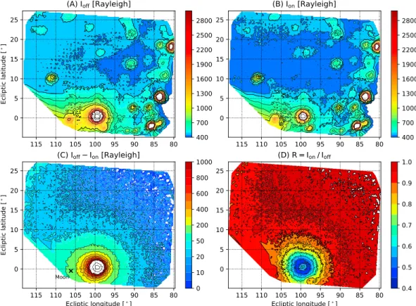
Figure 4 shows the data obtained on 24 January 1997 in the form of four sky maps: plot (a) presents the intensity Ioffwith the hydrogen cell turned off, plot (b) presents the intensity Ionwith active hydrogen cell, plot (c) shows the difference Ioff − Ionof the two previous intensity maps, and plot (d) presents the reduction factor R = Ion∕Ioff. According to the data in Figures 4c and 4d, it can be concluded that the extent of the exosphere is at least 10◦, which corresponds to a distance ∼40 RE. Looking at Figure 4a, besides the geocorona centered near an ecliptic point (longitude𝜆 ∼99◦, latitude𝛽 ∼ +1◦), there are plenty of “islands” of light, which are also present when the H cell is activated (plot b). These are due to some hot stars (i.e., T > 10, 000 K) with UV flux in the bandwidth of the detector (110–160 nm). Actually, the comparison with a UV star catalog allowed to identify all of the brightest and to detect that there was a slight discrepancy (∼1◦) between the actual coordinates in the sky and the position of these blobs of light given by the geometry pipeline (mainly a lon-gitude shift). This is probably due to a small mechanical misalignment between the SU+Z SU with respect to the SOHO spacecraft, which went unnoticed up to now. Also, the actual position of SOHO as seen from Earth was computed from JPL Horizons ephemeris online software (https://ssd.jpl.nasa.gov/horizons.cgi). Therefore, the position of the Earth as seen from SOHO was also computed and compared to the center of light of the geocorona of Figure 4. We found the same discrepancy as for the stars, as expected. Therefore, all measurements were reassigned new coordinates to account for the detected shift. Note that the image of one star, with a total diameter of ∼3◦, exceeds the nominal spatial resolution of 1◦(single pixel). This is because of optical aberrations introduced by MgF2lenses, which are wavelength dependent as the index of refraction
(Bertaux et al., 1995) and minimal at 121.6 nm by design of the MgF2lenses. At the distance of the Earth from
SOHO (∼230 RE), 1◦covers ∼4.1 RE. The direction to the Moon on 24 January 1997 (𝜆 = 106.15◦,𝛽 = −0.49◦) is marked by the black cross in Figure 4c, the SOHO-Moon distance is ∼290 REand SOHO-Earth-Moon angle is 144.68◦, which means that the Moon is on the opposite side from the Earth on this particular date, so the influence of the lunar gravity on the observed intensity distribution can be safely neglected.
Figure 4. The Solar and Heliospheric Observatory/Solar Wind Anisotropies data for 24 January 1997. (a) The intensity
Ioffwith the hydrogen cell turned off; (b) the intensity Ionobserved with active hydrogen cell; (c) is the difference (Ioff−Ion) of the maps (a) and (b); (d) the reduction factor R = Ion∕Ioff. The white areas are due to the exceeding of the upper limit of intensity in the color bar. The direction to the Moon is marked by the black cross on the plot (c). The polar axis of the Earth projected in the plane of the figure is not far (within 10◦) from the ecliptic latitude axis direction. The North Pole of the Earth is at a higher ecliptic latitude than the center.
We may see on the map of differences Ioff −Ion(Figure 4c) that the stars have disappeared. This is because
the H cell has an equivalent width of absorption of about ∼10−2nm, negligible with respect to the star
continuum 110–160 nm. The H cell has no effect on stars, and they disappear in the difference Ioff −Ion.
From the sketch of Figure 3, it can be seen that SOHO is away from L1on one side. As a result, on the maps
of Figure 4, the geotail is seen on the left side of the Earth, while the “sunny side” of the geocorona is seen on the right side. On the left side, the LOS is cutting the geotail further out than the nearest point to Earth along the LOS. This may introduce an uncertainty within the hypothesis of spherical symmetry of the exosphere that we will use in section 5 to retrieve the radial profile of H atoms in the exosphere and only the right side of the geocorona will be kept for further analysis.
As can be seen in Figures 2b and 2c, there is a band (about 40◦wide) along the ZDSC where the H cell is absorbing some of the IP emission. At first glance, the geocorona seems to be out of this region. However, a close examination of Figure 4c shows some enhancement of Ioff − Ionin the left part of the figure, with ecliptic longitudes𝜆 > 110◦. This is a contribution of the ZDSC band edge, where the H cell may still absorb a little of the IP sky background. As described in Appendix A, we have estimated the IP intensity absorbed by the H cell in the FOV. On a full-sky map recorded 1 day before (23 January), we have compared at latitude 31◦(where the contribution of the geocorona is negligible) the observed absorbed intensity to the prediction of a full model of the IP line shape and effect of the H cell (Figure A1). We had to multiply our model by a scaling factor 1.7 to reproduce the observed IP absorbed intensity. The scaled model of absorbed intensity was then calculated over the FOV of the geocoronal map (Figure A2b) and was subtracted from the original map of ID
off−I
D
on(Figure A2c) to get the pure geocoronal data plotted in Figure A2d. The band of intensity
on the left side has disappeared, even the most external isophotes are more roundish. Only a small artifact due to stray light from SOHO is still present on the lower left corner. Still, we have restricted the analysis of the pure geocoronal intensity to the right side area of the sky with ecliptic longitudes𝜆 smaller than the
longitude𝜆Eof the Earth's center (𝜆 < 𝜆E). There, the contribution of the IP difference is less than 4 R at distances>40 RE. Though it is not visible on the final difference map (Figure A2d), there is still some star contamination because of some high countings. The points measured near a known star will be discarded. The use of the H cell allows assigning the Ioff −Iondifference entirely to the geocorona, after correction of
H cell IP difference and star avoidance. This will allow to determine the intensity distribution of geocoro-nal emission up to unprecedented distances, and to derive the H density by an onion-peeling technique (a numerical way to operate the inversion of Abel transform) in the outer part of the geocorona, which is opti-cally thin (OT): the intensity in the LOS is directly proportional to the integrated number density of H atoms along the LOS. These density retrievals may be done (almost) independently of any model and should be useful for a better description of the extent of the geocorona, and for space operations planning purposes. For instance, if one decides to put a spectrometer in orbit to observe the Lyman-𝛼 emission of the IP medium, it is important to put the instrument outside of the geocorona, or at least to know what is the geocoronal intensity as a function of distance of the LOS to the Earth. However, it was felt reasonable to also compare our data to a model, in order to understand the physical parameters governing the H distribution in the exosphere. Such a model is described in the next section.
3. Kinetic Model of the Geocorona
The effect of radiation pressure on H atoms in the exosphere was computed by several authors in the past (Beth et al., 2016; Bishop & Chamberlain, 1989, and references therein). In (Beth et al., 2016) a Hamiltonian formalism is used to compute the evolution of various kinds of orbits under the effect of radiation pressure. They did not consider the effect of ionization, which effectively kills one H atom after some time. For the analysis of the SOHO/SWAN data, a numerical model of the exosphere was developed, based on a kinetic equation containing the ionization.
In this section we introduce a description of the kinetic model of the H atoms distribution in the geocorona that we used in our calculations. The kinetic approach is based on the concept of velocity distribution function. The distribution of the H atoms in geocorona is described by a kinetic equation:
𝜕𝑓(r, v, t) 𝜕t +v ·𝜕𝑓(r, v, t)𝜕r + F mH ·𝜕𝑓(r, v, t) 𝜕v = −𝛽(r, t) · 𝑓(r, v, t), (1)
where f(r, v, t) is the velocity distribution function, r the geocentric radius vector, v the individual velocity of an atom, t the time, mH the mass of H atom, F the resultant force acting on the atom, and𝛽(r, t) the effective ionization rate. The losses of atoms can be caused due to the following processes: charge exchange on solar protons (H + H+→ H++ H) and photoionization (H + h𝜈 → H++ e). In general, the total effective
ionization rate varies with time t, distance from the Sun and heliolatitude𝜆, but in our calculations we used a simplified model of the constant ionization rate𝛽 = 7 × 10⁻⁷s−1, which was obtained by averaging
the total ionization rates at 1 AU and zero heliolatitude in 1996–1998 presented by Bzowski et al. (2013). We admit that the ionization is strongly dependent on the solar conditions and that the actual rates for the dates when the special geocoronal observations were performed (24 January 1996, 1997, and 1998) differ from the value used in our calculations (the difference is less than 13%). Nevertheless, the main objective is not to perform the most precise calculations of the exosphere but to show qualitatively that the effect of the ionization should be taken into account. It should also be noted that the charge exchange with solar wind protons should be taken into account only at high altitudes (outside the magnetosphere). However, our calculations show that ionization is most important at the highest altitudes, so we use a constant value of the ionization rate everywhere in the computational domain for the sake of simplicity. The change in the number of particles due to elastic collisions can be neglected because of the large mean free path of the atoms in the exosphere; that is, we assume that Knudsen number Kn≫ 1.
We consider a motion in the Earth reference frame that rotates at the angular rate of the Earth's rotation around the Sun. In this reference frame, the Earth stays at rest and the vector of angular velocity pointing to the axis of rotation that is perpendicular to the solar ecliptic plane. The resultant force F acting on the atom in this frame can be expressed as follows:
Table 1
Intensities Measured at 7 REfor the Three Data Sets (OGO-5, LAICA, and SWAN), As well As Indicators of Solar Activity, Scattering Angle, Scattering Angle Factor, the Excitation Rate g, and Its Value g∗at Earth at the Date of Observation
Instrument OGO-5 LAICA SWAN SWAN SWAN
Year of observation 1968 2015 1996 1997 1998
Date of observation 5 March 9 January 24 January 24 January 24 January
Distance of instrument 24 2,348 234 236 225
to the Earth's center (RE) Solar activityFa
10.7 147.7 135.7 71 72 94
Total solar Lyman-𝛼lineb 4.89 5.03 3.66 3.55 4.10
(1011photons·cm−2·s−1)
Solar flux f at line centerc 4.37 4.52 3.08 2.96 3.53
(1012photons·cm−2·s−1·nm−1)
Excitation rate g (10−3s−1) 2.37 2.46 1.67 1.61 1.92
Ratio g∗∕gd 1.02 1.03 1.03 1.03 1.03
Ratio𝜇of radiation pressure 1.32 1.37 0.93 0.89 1.06
to solar gravitatione
Mean scattering angle𝜃(◦) 128 58 155 155 155
Scattering function factor 1.01 0.99 1.12 1.12 1.12
Average Lyman-𝛼intensity 1,300 2,040 1,701 2,405 2,929
at 7 RE(Rayleigh)
Integrated slant density N 5.31 8.13 8.83 12.95 13.22
at p = 7 RE(1011cm−2)
Note. LAICA = Lyman Alpha Imaging Camera; SWAN = Solar Wind Anisotropies; OGO-5 = Orbiting Geophysical
Observatory number 5.
aTaken from https://omniweb.gsfc.nasa.gov/ow.html website. bTaken from http://lasp.colorado.edu/lisird website. cDerived from the relationship established by Solar Ultraviolet Measurements of Emitted Radiation/Solar and
Heliospheric Observatory (Emerich et al., 2005). dTo account for Sun-Earth distance. e𝜇 = f∕f
0, where f0 =
3.32 × 10¹²photons·cm−2·s−1·nm−1(Bertaux, 1974).
F = FE,g+FS,p+FS,g+Fcen+Fcor, (2)
where FE,gand FS,gare the Earth's and solar gravitational attractive forces, FS,pthe solar radiative repulsive
force, and the last two terms correspond to the inertial forces: centrifugal and Coriolis forces, respectively. In a close proximity to the Earth center, the solar gravitational force and centrifugal inertial force compensate each other, that is, FS,g + Fcen ≈ 0, and the Earth's gravitational force is dominant. At the same time, at
far distances from the Earth (∼100 RE) the sum FS,g + Fcendiffers from zero (|FS,g + Fcen|∕|FE,g| < 0.08)
but, as our calculations have shown, they can be neglected because an inclusion of these forces changes the distribution of atoms in the exosphere insignificantly. As for the Coriolis force Fcor, it also differs from
zero at such distances from the Earth (|Fcor|∕|FE,g| ∼ 0.3). Nevertheless, Coriolis force can also be neglected
according to our calculations. The motion of atoms at far distances from the Earth is mainly ruled by the solar radiative repulsive force (|FS,p|∕|FE,g| ∼ 5 at 100 RE). Thereby, we did not take into account the solar gravitational, centrifugal, and Coriolis forces in our calculations for the sake of clarity. For the solar radiation pressure we assumed that FS,p = −𝜇FS,g, where𝜇 = |FS,p|∕|FS,g|. In the general case, the parameter 𝜇 depends on the time t, heliolatitude𝜆, and the radial component of the atom's velocity vr, but in our research we use a constant value𝜇 = 0.9 for near minimum solar cycle conditions (1996–1998) and zero radial atom's velocity and heliolatitude (for details see Katushkina et al., 2015) that is slightly different from the actual values for 24 January 1996, 1997, and 1998 (𝜇 = 0.93, 0.89, 1.06, respectively; see Table 1).
In the frame of the kinetic theory the moments of the velocity distribution function at point (r, t) ∈ R4are
the following values:
• zero velocity distribution function moment—number density n:
• first velocity distribution function moments—components of the bulk velocity Vi: Vi(r, t) =
1
n(r, t) ∫ 𝑓(r, v, t)vidv; (4)
• second velocity distribution function moments—kinetic temperatures Ti≡ Tiiand correlation coefficients {Tij, i ≠ j}: Ti𝑗(r, t) = mH n(r, t)kB∫ 𝑓(r, v, t) ( Vi(r, t) − vi ) ( V𝑗(r, t) − v𝑗)dv. (5)
In formulas (3)–(5) we use the following notations: i ∈ {x, 𝑦, z}, where XYZ are some orthogonal coordinate system; kBthe Bolzmann constant; dv = dvx·dvy·dvz; and integration is performed all over the velocity space v = (vx, v𝑦, vz) ∈R3.
3.1. Method of Characteristics
The kinetic equation (1) is a linear partial differential equation that can be solved by a method of character-istics. A characteristic is a curve in the phase spaceR6of coordinates and velocities, and it is defined by the
following equations: {dr dt =v, dv dt = F mH. (6)
Along this characteristic the velocity distribution function f(r, v, t) must satisfy the following equation: d𝑓(r, v, t)
dt = −𝛽(r, t) · 𝑓(r, v, t), (7)
and the solution of that equation can be written in the following form: 𝑓(r, v, t) = 𝑓c(rc, vc) ·e−I, I = ∫
t tc
𝛽(r, t)dt, (8)
where fc(rc, vc)is the velocity distribution function of the H atoms at the inner boundary of the computa-tional domain (exobase) that is the exterior of the Earth centered sphere with radius Rexo; rc, vc, tcare the position, velocity, and time, respectively, when the atom crossed the inner boundary and enters the com-putational domain; I is a loss integral due to ionization processes. The integration is performed along the atom's trajectory that satisfies the system of equations (6) of the characteristic curve.
By solving the kinetic equation (1) with a specific boundary condition fc(rc, vc), we can find the value of the velocity distribution function everywhere in the computational domain. This modeling approach is equiva-lent to the use of Liouville's theorem, which states that, in absence of collisions, the density in phase space is constant along a dynamical trajectory. The “characteristic” mentioned above is a dynamical trajectory. In order to compute at a given point r the density, one has to scan all possible velocity vectors v, check if the corresponding trajectory cuts the exobase (if it does not cut, the particle does not exist), and compute the corresponding density in phase space at the origin (the boundary condition). The extinction by ionization must be computed, as well as the actual trajectory, taking into account the constant solar Lyman-𝛼 radiation pressure. In the section below we specify the boundary condition that is used in our modeling.
3.2. Boundary Condition
The boundary condition in the model is set at the lower boundary of the exosphere that is called exobase and assumed to be the Earth centered sphere with radius Rexo = 6871km (500 km above the Earth's surface). We use a boundary condition in the form of the Maxwell distribution function
𝑓c(v) = nexo (√𝜋cexo)3·exp ( − v 2 c2 exo ) , cexo= √ 2kBTexo mH . (9)
Figure 5. The H density distribution as a function of radial distance for three models with the same exobase conditions
nexo =1.2 × 105cm−3, Texo=1000K. Black solid line presents Model 1—classical Chamberlain model without
satellite particles (𝜇 = 0,𝛽 = 0)—magenta dashed line (Model 2) is the Chamberlain model with ionization (𝜇 = 0,
𝛽 = 7 × 10⁻⁷s−1). The distribution using Model 3, which includes both the effect of ionization and radiation pressure
(𝜇 = 0.9,𝛽 = 7 × 10⁻⁷s−1), was calculated along the Earth-Sun line (yellow dash-dotted curve), north-south line
(orange dashed line), and in the anti-Sun direction (red dotted line). The bottom panel shows Model 2 to Model 1 (blue solid line) and Model 3 to Model 2 ratios in different directions. Those ratios indicate the formation of a bulge of H atoms by solar radiation pressure in the range 2–30 REon the Sun side (𝜃= 0◦), less pronounced on the side (𝜃= 90◦), and an excess at all distances, forming a geotail in the antisunward direction (𝜃= 180◦).
with number density nexo ∼ 105cm−3, zero bulk velocity and temperature Texo ∼1000K. It is important
to note that in reality the number density and temperature distributions at the exobase are not uniform. Nevertheless, we use a uniform boundary condition as a first order approximation.
3.3. The Effect of Ionization and Radiation Pressure on the Radial Density Profiles
Figure 5 shows the H density distribution as a function of radial distance for three models with the same exobase conditions nexo = 1.2 × 105cm−3, T
exo= 1000 K. Model 1 has no ionization and no radiation
pressure; therefore, it is a classical model of Chamberlain, without satellite particles. Model 2 includes in addition the effect of ionization with𝛽 = 7 × 10⁻⁷s−1. As expected, the effect of ionization is more important
as large distances. The ratio of Model 2/Model 1 is indicated at bottom of Figure 5. The values of losses due to ionization at 50 and 100 REare 21% and 32%, respectively. Model 3 has the same ionization as Model 2, but now the effect of the radiation pressure on hyperbolic and ballistic H atoms is included for the case𝜇 = 0.9. It is to be noted that Model 3 has no longer a spherical symmetry and the number density depends not only on the distance to the Earth's center but also on angle𝜃 between the Earth-Sun direction and radius vector (cylindrical symmetry). In Figure 5 the H density distribution for Model 3 was computed along the Earth-Sun line (𝜃 = 0◦, yellow dash-dotted curve), north-south line (𝜃 = 90◦, orange dashed curve), and in the anti-Sun direction (𝜃 = 180◦, red dotted curve). The ratio of Model 3/Model 2 is also plotted at the bottom of Figure 5. The effect of the radiation pressure for𝜃 = 0◦is that the density is depleted at large distances, and increased (up to factor ∼ 2.7 at 12 RE) at shorter distances: the exosphere is compressed creating a relative bulge of atomic H in the region from 2 to 30 RE. This effect can also be seen for north-south direction (𝜃 = 90◦) but
it is significantly weaker (increase up to factor ∼ 1.6 at 10 RE) than for𝜃 = 0◦. The ratio of Model 3/Model 2 for the anti-Sun direction (𝜃 = 180◦) is increasing with the geocentric distance and reaches a factor ∼ 7 at 100 RE. The atoms on the “dark” side of the exosphere are forming the so-called “geotail,” the region of the increased hydrogen number density, which can be reproduced using our model which includes radiation pressure (Bertaux & Blamont, 1973; Thomas & Bohlin, 1972). Our present numerical results are fully in line with the results of Beth et al. (2016) shown in their Figure 3, where they find a bulge of factor 2.5 on the dayside.
4. Comparison of SWAN Measured Geocoronal Intensities With Models and
other Observations
4.1. Comparison With Numerical Model Results
As the initial data for the comparison, we use the difference (ID
off−I
D
on) of intensities (superscript “D” denotes
the data). This approach allows excluding radiation from stars and other external sources (e.g., the IP back-ground and the reflected solar radiation from parts of the SOHO spacecraft), which makes the data much more suitable for subsequent processing. In principle, the stars have disappeared in the data (ID
off−I
D
on), but
as said before the uncertainties of measurements in the directions of stars are still sometimes rather large (due to high count rates). The data points that correspond to stars were removed, which reduces the dis-persion of intensities (original disdis-persion not shown here; for more details see the supporting information). In addition, we subtracted from the data the IP intensity (Ioff− Ion), which was estimated using the model
(see details in Appendix A), and exclude the “asymmetric” part of the data that corresponds to the lines of sight with longitudes larger than the longitude of the Earth, where the assumption of local spherical sym-metry may no longer be verified because of the geotail. Therefore, it can be assumed that the remaining data depend only on the impact parameter of each particular LOS (local spherical symmetry). By doing this, we implicitly assume an ecliptic north-south symmetry of the exosphere that was previously reported by Kameda et al. (2017) and can also be seen in SWAN data (see, e.g., Figure A2d).
To calculate the backscattered solar Lyman-𝛼 radiation from the geocorona, we used the radiation trans-fer model in the OT medium approximation. Zoennchen et al. (2010) estimated that the H densities are low enough at geocentric distances r > 3REto make valid the assumption of OT conditions. As indicated in Figure 6, our measured intensities start to be smaller than the OT calculations below 3REfor a model adjusted at large distances, confirming their estimate. For the model, we have computed the total intensity, the line profile of the emission integrated along the LOS, and the absorption effect of the H cell.
One SWAN hydrogen cell, when activated, is filled with a cloud of atomic hydrogen gas with a temperature Tc = 300K and optical thickness𝜏c = 3.4 as determined from ground calibrations and in-flight analy-sis. Using our model of the exosphere we performed the simulations of intensities IM
offand I
M
onobserved by
SOHO/SWAN, as well as the reduction factor RM=IM
on∕IoffM (superscript “M” denotes the model).
Figure 6 presents the dependence of the difference of intensities (Ioff − Ion) on impact parameter p (per-pendicular distance of the LOS to Earth's center): black dots show the SWAN data obtained on 24 January 1997, red solid line is the averaged data, blue and cyan dashed lines are the results of model simulations with parameter𝜇 = 0, number density nexo = 1.2 × 105cm−3and temperatures T
exo = 1000K and
Texo = 1200K at the exobase, respectively. The yellow solid line is the numerical curve with solar
pres-sure included (𝜇 = 0.9) and parameters nexo = 1.3 × 105cm−3, Texo = 1000K. According to Figure 6, it
is clear that the models without solar pressure (blue and cyan curves) cannot reproduce the data at short (3–10 RE) and far distances from the Earth at the same time. By contrast there is a good quantitative agree-ment between the SOHO/SWAN data and our numerical simulations for the case𝜇 = 0.9 (yellow solid line) at impact parameters from 3 REup to 30–50 RE. Below ∼3 REthe model increases fast toward the Earth while the data flatten. There are two reasons for the flattening of the data. The most important is self-absorption (SA) along the LOS, which tends to limit the Lyman-𝛼 intensity (saturation effect). The second reason for flattening is due to the finite SWAN FOV of 1◦, or 4 RE, which blurs out the strong maximum intensity on the disc of the Earth.
Comparing the model with𝜇 = 0.9 with models with 𝜇 = 0, we may qualitatively understand the effect of radiation pressure on the exosphere. It decreases the H density above 15 REand increases the density below
Figure 6. The dependence of the difference of intensities (Ioff−Ion) on
impact parameter p: black dots show the SWAN data obtained on 24 January 1997, red solid line is the averaged data, blue and cyan dashed lines are the results of simulations with parameter𝜇 = 0, number density
nexo = 1.2 × 105cm−3and temperatures T
exo = 1000K, and
Texo =1200K at exobase, respectively. The yellow solid line presents the result of calculations with solar pressure included (𝜇 = 0.9) and parameters nexo = 1.3 × 105cm−3, T
exo =1000K. Below 3 REthe data
diverge from the models due to multiple scattering, not included in the modeling. The typical uncertainties of the averaged data at 3, 10, and 100 REare∼15, 2, and 0.2 R. SWAN = Solar Wind Anisotropies; SOHO = Solar and Heliospheric Observatory.
15 RE, creating a (relative) bulge of H density in the region 3–15 RE. The whole effect is on ballistic and hyperbolic particles. It is rather spectac-ular, in view of the short time spent by a particle in the exosphere (a moderately hyperbolic particle needs ∼3 hr to reach 15 RE). Beth et al. (2016) have investigated the effect of radiation pressure on H atoms in satellites orbits. They found that if the particle approaches the Sun-Earth line, it will decay to the exobase. There is a region of stability for these atoms which does not include the segment Earth-Sun line.
In the present paper, we wish to report on the radial profile and extension of the geocorona, both with Lyman-𝛼 intensities and H number density as a function of geocentric distances. Figure 6 shows indeed a remark-able extension of the geocorona up to ∼100 RE(about twice the distance Earth-Moon), clearly established thanks to the H cell absorption. 4.2. Determination of the SWAN Geocoronal Emission Lyman-𝜶 Intensity
What is plotted in Figure 6 is the emission absorbed by the cell ID
off−I
D
on,
and we wish to determine Ig,off, the geocoronal emission. The Lyman-𝛼
intensity I registered by SWAN in the region of geocorona consists of two main terms: the IP background Ibgand the radiation from geocorona Ig, that is, I = Ibg + Ig. In order to separate the exospheric radiation from the background, a first approach was applied (strategy 1) as described in the following. The intensity of the backscattered solar Lyman-𝛼 radiation from the geocorona Ig,offwas calculated by the following formula:
Ig,off=I D off−I D on 1 − RM , (10)
where RM(𝜇, Texo)is the reduction factor that was calculated using our model (strategy 1). This formula is valid since we have subtracted from the original difference data the small contribution of absorbed IP background.
Figure 7. The reduction factor profiles that were calculated using the geocorona model with different values of𝜇and
Texo. The blue and cyan dashed lines correspond to the case of𝜇 = 0, Texo= 1000 K and Texo= 1200 K, respectively. The yellow solid line was obtained using the model with solar pressure included (𝜇 = 0.9) and Texo= 1000 K. The increase of the reduction factor above 20 REis due to a spectral shift of the observed atoms outside of the H cell absorption, induced by a change of the velocity vector of H atoms through the bending of trajectories by radiation pressure as could be verified in the model.
Figure 8. Geocorona intensities obtained by different strategies. The strategy 1 resulting intensity curve (with RM computed for Texo= 1000 K and𝜇= 0.9) is displayed as a thick green dashed curve. The same model gives the total intensityIMg,off(with nexo = 1.3 × 105cm−3) indicated by the yellow dashed curve. The strategy 2 was also used to
derive the geocoronal intensity, by subtracting estimates of the interplanetary background Ibg. Either a uniform sky background of 420 R was subtracted (thick blue line) or a model of the sky background was subtracted, after
adjustment by multiplying by a factor of 1.5 (dash-dotted cyan line). The typical uncertainties of the averaged data at 3, 10, and 100 REare∼10, 1, and 0.15 R. SWAN = Solar Wind Anisotropies; SOHO = Solar and Heliospheric Observatory.
The models of the reduction factor for different values of𝜇 and Texoare presented in Figure 7. They differ
somewhat, and there is an associated uncertainty when selecting the model to use for dividing by 1 − RMto estimate the unabsorbed intensity Ig,off. But at far distances (p > 40RE), the difference is not so large (∼ 10%), when comparing 1 − RM≈0.8 for 𝜇 = 0, Texo = 1000K model, and ≈ 0.75 for 𝜇 = 0.9, Texo = 1000K.
The resulting SWAN intensity curve (with RM computed for T
exo = 1000 K and𝜇 = 0.9) is displayed as a
thick green curve in Figure 8. The same model gives the total intensity IM
g,off(with nexo = 1.3 × 105cm−3)
indicated by the yellow dashed curve. Data and model curves show the same similarities and differences as the two corresponding curves in Figure 6, which is normal since they have been obtained by the same division by 1 − RM. Therefore, the same comments as for the corresponding curves of Figure 6 do apply. The original SWAN data Ioffare plotted as black dots in Figure 8. A second strategy was also used to derive
the geocoronal intensity, by subtracting estimates of the IP background Ibg. Either a uniform sky
back-ground of 420 R was subtracted (strategy 2a, thick blue line in Figure 8) or a model of the sky backback-ground was subtracted, after adjustment by multiplying by a factor of 1.5 (strategy 2b, dash-dotted cyan line). To calculate the sky background, we used the model described by Katushkina et al. (2015) with boundary con-dition at 70 AU, which was derived using the global model of the solar wind and Local Interstellar Medium interaction (Izmodenov & Alexashov, 2015). This model differs from the one that was used to compute the absorbing effect of the H cell (Appendix A), and this is why the adequate scaling factor is quite different for the two models. At distances> 50REthis second variant (subtraction of a model) certainly makes more sense, because the geocorona is seen over an angle (diameter) of 25◦at 50 REand 50◦at 100 RE, and clearly, the sky background is not uniform over such angular spans. A straight line is also plotted, corresponding to a −2 power law of the intensity with respect to the impact parameter. It runs nicely parallel to the SWAN derived intensity: at large distances, the decrease of the geocoronal Lyman-𝛼 intensity may be described to first order as a −2 power law.
In the region from 3 to ∼ 30RE, there is a discrepancy between the actually measured geocoronal intensities when the cell is off, Ig,off(with a sky background subtracted from black dots yielding the blue curve) and the
green curve, estimate of Ig,offobtained from the division of measurements (IDoff−I
D
Figure 9. Comparison of the Lyman-𝛼intensity extracted from SWAN data obtained on 24 January (1996, 1997, and 1998) with two other data sets (OGO-5 and LAICA). The blue, green, and red solid lines with dots represent composite geocorona intensity curves for 1996, 1997, and 1998, respectively. The black line with dots is the data obtained by OGO-5. The LAICA data for different directions presented by the cyan, magenta, yellow, and gray solid lines (for details see Kameda et al., 2017, Figure 3). The typical uncertainties of the SWAN composite data at 3, 10, and 100 RE are∼10, 1, and 0.3 R. The average (between 1997 and 1998) geocoronal Lyman-𝛼intensity at 100 REis 5.91±0.33 R. SWAN = Solar Wind Anisotropies; OGO-5 = Orbiting Geophysical Observatory number 5; LAICA = Lyman Alpha Imaging Camera.
curve (data) is larger than our best model by ∼57% and ∼45% at 3 and 20 RE, respectively. In other words, it means that our best model reproduces well the difference Ioff − Ion, but not the values of Ioff(neither
Ion). Clearly, if some intensity not at all absorbed by the H cell were added to the model, then both Ioff and Ioncould be fitted simultaneously. In fact, this would be the case of H atoms in satellite orbits, with
velocity vectors more parallel to the LOS than hyperbolic or ballistic ones. The Chamberlain models that we have used here (modified by radiation pressure) do not include such satellite particles, but they actually do exist, according to the analysis of data acquired by OGO-5: H cell absorption measurements up to 7 RE (Bertaux, 1978), and intensity measurements obtained in 1969–1970 between 5 and 16 REduring special spin maneuvers of OGO-5 (Bertaux & Blamont, 1973). This topic of satellite particles will be discussed further later on. For a rough estimate, the relative excesses of intensities ∼57% and ∼45%, respectively, at 3 and 20 RE may be translated into equal local H density excesses at the same radial distances, inasmuch as the main contribution along a LOS comes from the nearest point to the center of the Earth. It gives an idea of the important contribution of H atoms in satellite orbits to the total H density. And this is likely a lower limit, because some atoms in satellite orbits (with Doppler shift velocity<3 km/s; the equivalent width of the H cell is ∼5.5 km/s) might produce a Lyman-𝛼 emission absorbed by the H cell.
4.3. Comparison With Some Other Geocoronal Observations
The geocoronal Lyman-𝛼 intensity extracted from SWAN data obtained on 24 January (1996, 1997, and 1998) are now compared with two other data sets (Figure 9). The SWAN intensity curves were obtained by a composition of two strategies: at small distances (below 10 RE) the result of strategy 2b was used, and at far distances (above 20 RE) the strategy 1 was applied. In between a nudging process was done. This approach was used since the true reduction factor is not well reproduced by the model at small distances and therefore strategy 2b is more valid, and the true value of IP background cannot be estimated with high accuracy at large distances and therefore strategy 1 is favored. The nudging process was made for the three years for consistency; however, for 1996 the nudging process had no effect because the two strategies yielded the same intensity curves. In other words, for 1996 both the intensity Ioffand Ioncould be reproduced by the model,
which means that the reduction factor on the data was the same as predicted by the model with radiation pressure.
The oldest data set for the comparison was collected on 5 March 1968 by experiment E-22 on OGO-5, from a distance of 153,000 km (Bertaux, 1978). The experiment was placed in a rotating box, allowing to record the map of Figure 1. However, the rotation was commanded off during two hours, in order to collect the data in a single vertical plane (not cutting the Earth's shadow) with a resulting high SNR. The scanning mirror allowed measuring the intensity up to a distance of 7RE. An estimate of the IP background was subtracted, based on posterior observations of the sky during spin maneuvers (Bertaux, 1978). The calibration factor of OGO-5/E-22 was derived by observations of the geocorona, which absolute H number densities in the exosphere were obtained from OSO-5 H absorption measurements on the center of the solar Lyman-𝛼 line (therefore, absolute H column density numbers).
The second data set is the one collected from the Lyman-𝛼 image LAICA instrument on 9 January 2015 as described in section 1. The calibration factor of LAICA was derived from one observation of the IP back-ground and absolute intensities delivered by SWAN (Kameda et al., 2017). However, a recent comparison of the SWAN and SPICAV data in 2008–2014 shows a degradation of the SWAN instrument sensitivity with ∼3.3 ± 0.9%/year. This preliminary work leads to a total degradation of ∼46 ± 13% during the period of time from 2001 (when cross calibration with HST were made; see ; Quémerais et al., 2013) to 2015, assuming that the degradation is the same over that period. The absolute values of SWAN intensities used by Kameda et al. (2017) should be multiplied by a factor of 1.85 ± 0.44. We are reproducing in Figure 9 the four curves extracted from Figure 3 of Kameda et al. (2017) in four different planes with new normalization (multiplied by 1.85).
In the region from 4 to 7 REwhere they overlap, the OGO-5 and LAICA data set are parallel, LAICA being brighter than OGO-5 by a factor of 1.57 at 7 RE. Such a distinction may be due to a genuine difference of the hydrogen exospheric density. Both data sets were collected during a solar maximum. However, other factors are involved in the passage from Lyman-𝛼 intensity to H density as described in equations (11)–(15): the exciting solar flux at line center, the Sun-Earth distance, the nonisotropic phase function of Lyman-𝛼 scattering, and the calibration factor of each instrument. In Table 1 we summarize the intensities measured at 7 REfor the three data sets, as well as indicators of solar activity, scattering angle, scattering angle factor, the excitation rate g and its value g∗at Earth at the date of observation.
The scattering phase function𝛷(𝜃) at Lyman-𝛼 is not strictly isotropic and depends on the scattering angle 𝜃 = 𝜋− phase angle (Brandt & Chamberlain, 1959):
Φ(𝜃) = 1 +1 4
(2 3−sin
2𝜃). (11)
To compute the excitation rate g relevant for the dates of observations, the flux of the total solar Lyman-𝛼 flux is taken from the Colorado database (http://lasp.colorado.edu/lisird), and the statistical relationship between total flux F and flux at line center f established by Emerich et al. (2005) is used to derive the flux at line center: 𝑓 1012s−1·cm−2·nm−1 =0.64 ( F 1011s−1·cm−2 )1.21 ±0.08. (12)
Then, the excitation rate is obtained by multiplying f by the integrated cross section𝜎𝜆of one single H atom:
g =𝑓 · 𝜎𝜆, (13) 𝜎𝜆= ∫ +∞ 0 𝜎(𝜆)d𝜆 = ( 𝜆2 c ) ∫ +∞ 0 𝜎(𝜈)d𝜈 = ( 𝜆2 c ) 𝜋e2 mec𝑓12=5.445 × 10 −15cm2Å. (14)
In the formula above, the two c must not be mixed into a c2: the first one must be in the same unit length as
𝜆, the second one is in centimeters per second.
In the frame of the OT approximation, and applying formulas (11) to (15) to the intensities measured by the three instruments at 7 RE, a slant density N of H atoms may be retrieved for a LOS at 7 REof impact
parameter and is indicated in Table 1. The LAICA value of N is 1.53 times larger than the OGO-5 value NOGO −5 = 5.31 × 10¹¹atoms/cm2. We might assign this difference to natural variability of the exosphere
at a similar high solar activity, and/or to uncertainties in the relative calibrations of the two instruments. We now compare the SWAN data taken in 1997 near a solar minimum to LAICA. At the distance of 7 RE, SWAN measured a higher intensity of ∼ 2400 R (from strategy 2b), versus 2040 R for LAICA (Table 1). When all relevant factors are accounted for, the slant density of SWAN (12.95 × 10¹¹atoms/cm2) at 7 R
Eis ∼ 1.59 times larger than the LAICA slant density. It can be noted from Figure 9 that at larger distances>20 RE, the SWAN and LAICA intensities become much more similar, implying also similar density distributions. Therefore, it seems clearly established from SWAN/LAICA comparison that at solar minimum, there is a substantial increase of the H exosphere in the range 4–10 RE, with much less difference at larger distances (smaller distances cannot be well observed by these two instruments).
A potential explanation for this bulge of hydrogen is the building up of a population of H atoms in satellite orbits during low solar activity. Collisions between neutrals were already considered by Chamberlain (1963) as a way to build up such a population. More important may be the role of charge exchange between H atoms on ballistic orbits with protons in the plasmasphere: these protons have an isotropic velocity distribution and when neutralized to become an H atom they have a good chance to be launched on a satellite orbit. Once there, their orbit will be modified by solar Lyman-𝛼 radiation pressure, until they collide again with the exobase, or are ionized by charge exchange with solar wind protons or EUV photo-ionization.
The description of the population of satellite particles by Chamberlain (1963) is that they are just completing locally the Maxwell-Boltzmann velocity distributions, but no more (up to a so-called Critical Satellite Radius RCS, above which only those coming from below do exist). However, as noted by Bertaux (1978), the actual
distribution of satellite particles is the result of production, evolution and destruction processes. In some regions where the collisions are infrequent, there could very well exist an “excess” of satellite particles, with respect to the limit of “completion” to Maxwell-Boltzmann distributions, as well as a deficit in other regions. For the OGO-5 solar max conditions, it was found (Bertaux, 1978) from the H cell measurements that at 5 RE, H atoms in satellite orbits were accounting for ∼45% of the total H density, with a lesser contribution below and above. According to the SWAN observations, their contribution could even be much more important during solar minimum. However, the analysis of the OGO-5 data was done by comparison with a model, not including solar radiation pressure: accounting for it might decrease the quantity of H in satellite orbits necessary to fit the observations since radiation pressure compress the exosphere on the dayside.
In our kinetic model, we explore the velocity space at one given geometrical point and calculated back in time its trajectory to find the phase space density in the Maxwell-Boltzmann distribution where the trajectory crosses the exobase. We found that some velocity vectors, which would correspond to a satellite orbit with no radiation pressure, were indeed cutting the exobase at some time before when the orbit was extrapolated back in time. Clearly, radiation pressure can change the status of a ballistic particle into a satellite particle, at least for many orbits, before being ionized, or put back to the exobase, or pushed to escape on a hyperbolic trajectory. A shown by Beth et al. (2016), radiation pressure is also very effective to put a satellite H atom on a ballistic trajectory and back to the exobase, for those atoms which approach the Earth-Sun line on the dayside. Therefore, with the effect of radiation pressure, the status of a satellite atom may be only temporary. We note that at solar minimum, the EUV solar flux is smaller, and the magnetopause nose is at a larger distance from the Earth, better protecting such a population of orbiting H atoms. This might explain partially the conspicuous difference observed in the exosphere between solar max and solar min conditions.
5. Retrieval of the H Density in the Exosphere From SWAN Data
The retrieval algorithm to go from measured intensities to local densities uses the assumption of the OT medium and a spherical symmetry of the geocorona, which makes it possible to use the fact that the observed intensity is proportional to the integral N(p) of hydrogen atoms number density along the particular LOS in cm−2: